Self-trapping transition for a nonlinear impurity within a linear chain
Abstract
In the present work we revisit the issue of the self-trapping dynamical transition at a nonlinear impurity embedded in an otherwise linear lattice. For our Schrödinger chain example, we present rigorous arguments that establish necessary conditions and corresponding parametric bounds for the transition between linear decay and nonlinear persistence of a defect mode. The proofs combine a contraction mapping approach applied in the fully dynamical problem in the case of a D-lattice, together with variational arguments for the derivation of parametric bounds for the creation of stationary states associated with the expected fate of the self-trapping dynamical transition. The results are relevant for both power law nonlinearities and saturable ones. The analytical results are corroborated by numerical computations.
I Introduction
The theme of discrete linear chains with embedded nonlinear impurity nodes is one of considerable interest within condensed matter physics. It emerges, for instance, within tight-binding descriptions of electron transport, where the nonlinear terms describe local interactions with vibrations at the impurity node [1], [2]. It also arises in the study of tunneling through a magnetic impurity connected to two perfect leads in the presence of a magnetic field [3]. It is also fairly widespread in the realm of nonlinear optics, where waveguides with practically linear and ones with essentially nonlinear characteristics can be constructed. This was proposed e.g. in [4]; however, notice that in that context linear and nonlinear waveguides were proposed to be interlaced in binary arrays. Here, instead, we have in mind a single nonlinear waveguide embedded in an otherwise linear array. Given this diverse array of physical setups, this subject was numerically examined in a wide array of studies [5, 6, 7, 8, 9], not only for the case of one but also for that of more embedded impurities. This topic has also recently seen a surge of renewed interest, due in part to the examination of eigenvalue problems and symmetry-breaking features in the presence of multiple linear or nonlinear impurity sites, and also due to the examination of gain/loss variants thereof [10, 11, 12, 13, 14].
While numerically the relevant dynamics is rather straightforward and directly tractable, on the analytical side, unfortunately, developments have been considerably less advanced. While it is possible to characterize the stationary states of the problem via the Green’s function techniques [7], and even (for specially constructed potentials) to capture symmetry-breaking effects via the demonstration of emergence of asymmetric states [10], little has been rigorously established about the dynamic problem. Assuming that initially, the excitation is placed at site of the chain, that is , the work of [8] was intriguing in that it established a particular diagnostic
| (1.1) |
with a clearly distinct behavior for different parameters (i.e., nonlinearity strengths ) of the system. The numerical (or physical) experiment at hand is as follows. Suppose we initialize the nonlinear site at unit intensity (the relevant amplitude can always be rescaled so that there is one parameter, either the strength of the nonlinearity or interchangeably the magnitude of the compactly supported –on a single site– initial data). We then monitor [in fact, in our case, we will not compute the relevant integral numerically starting from but rather from to exclude short term transient dynamics]. We then observe that for (which for the cubic nonlinear case is ), our diagnostic quantity tends to 0. On the contrary, for , the quantity remains finite and displays an increasing trend as increases [8].
In the present work, we initiate our investigations for establishing such a behavior from a rigorous perspective, and examine (both analytically and numerically) how the behavior is modified for different types of nonlinearities. In particular, we will focus on power law nonlinearities, as well as on saturable ones.
More specifically, we will consider the discrete nonlinear Schrödinger equation (DNLS), with the single nonlinear impurity in a -dimensional lattice, ,
| (1.2) |
where , and is the coupling between sites and .
Motivated by applications in the context of nonlinear optics [15], we shall concentrate on two examples of nonlinearities , namely the power-law nonlinearity
| (1.3) |
and the saturable nonlinearity
| (1.4) |
with the single site, unit intensity initial condition
| (1.5) |
indicated above. Note that here denotes in the -dimensional lattice.
We follow two different approaches: The first approach is based on the study of a nonlinear integral equation for , derived in section II. However, in this dynamical approach, we shall use a different diagnostic for self-trapping than (1.1), namely
| (1.6) |
Then, in section III, and in the case of the -dimensional lattice, we apply on the integral equation a contraction mapping approach, and prove the following: there exists a critical value , such that if , then . Although our rigorous result is restricted to the D-case, it is also suggestive of the numerically identified dynamical transition. Furthermore, it appears that the corresponding value for the saturable nonlinearity is greater than the one for the power nonlinearity. Next, by using an approximation near the linear regime of the system, we will rationalize an increasing behavior of the possible critical point for the power nonlinearity, as well as, unify our critical point estimates for the cubic and saturable case. We remark that the restriction in the dimension is imposed by integral divergence properties of the kernel of the integral map.
In section IV we discuss our second, variational approach. The latter is motivated by numerical results, illustrating that when is greater than the actual numerical value , is approaching a non-vanishing constant value. Such a convergence suggests that in the strongly nonlinear regime , and after a long time, that the dynamics of is approaching a stationary (i.e., standing wave) state. This, in turn, motivates us to discuss the possible existence of critical values on for the formation of stationary states. On the one hand, and under the light of the above assumption on the long time asymptotics, we work on the integral equation and derive critical values for the D and D cases, for both types of nonlinearities. On the other hand, the suggested dependence of the derived critical values on the dimension , motivates us to apply constrained minimization arguments on the stationary DNLS equation in the lattice , . Interestingly, the obtained critical values on (for the existence of such standing waves) both unify and extend the observations from the manipulation of the integral equation in the D and D cases, and demonstrate the following qualitative features: (a) In the case of the power nonlinearity, the critical value increases, as the nonlinearity exponent increases. (b) Both critical values for power and saturable nonlinearities, increase as the dimension of the lattice increases. (c) The critical value for the saturable nonlinearity is larger than the critical value for the cubic power nonlinearity.
In Section V, we present the numerical computations of the physical quantity , as well as for (1.6), and examine the self-trapping dynamical transition. The computations have been performed for lattice dimensions . In all cases, the numerical results confirm the existence of a dynamical transition. Furthermore, the numerical critical values for self-trapping share the above analytical trends, such as the dependence on the nonlinearity exponent, the type of nonlinearity, as well as, the dimension of the lattice with the critical points for the existence of stationary states that we present in section IV.
Finally, in section VI, we will summarize our findings and present our conclusions, as well as suggest some potential directions for future work.
The complementary section VII.1 includes for completeness, some basic properties of the eigenvalue problem for the discrete Laplacian on , supplemented with Dirichlet boundary conditions, while section VII.2 contains some special function properties of use to our stationary state calculations.
We should stress here that there are a few features that distinguish our results from earlier works discussed above that identified the full stationary family of solutions to the problem of a single defect (and even to that of multiple defects) within a linear lattice and that also numerically demonstrated the dynamical self-trapping transition, as discussed above. Here, not only is the self-trapping transition explored numerically for a variety of models (power or saturable nonlinearities) and a variety of dimensions (1D, 2D and even 3D) but importantly the transition is rigorously proven to exist in sufficiently high dimension (N=3) and additional arguments are given approximating its critical point in the different cases examined.
II Derivation of an integral equation for
In this section we will derive a dynamical, nonlinear integral equation for the evolution of . Let us consider first the case . We define the Fourier transforms
| (2.1) | |||||
| (2.2) |
where . Taking the Fourier transform (2.1) of Eq. (1.2), and assuming , we get the equation
| (2.3) |
where
| (2.4) |
is the dispersion relation. Now we take the Laplace transform of Eq.(2.3)
| (2.5) |
that is,
| (2.6) |
Then, we take the inverse Laplace transform of Eq. (2.6). The first term is the Laplace transform of . The second term is a product of two transforms, and therefore, its inverse is a convolution of and . Hence,
| (2.7) | |||||
Up to this point, the treatment is completely general. To obtain a specific result, we must use the exact form of the dispersion relation . In our case, . The last step is to take the inverse Fourier transform of Eq. (2.7). Using Eq. (2.2), the first term will be
| (2.8) |
that is,
| (2.9) |
Using the integral representation of the Bessel functions
| (2.10) |
the first term in Eq. (2.7) leads to .
For the second term in Eq.(2.7), we exchange the integrals over and and arriving to
| (2.11) |
Finally, putting everything together, we derive
| (2.12) | |||||
In particular, for we have
| (2.13) | |||||
or, equivalently,
For the -dimensional cubic lattice, the extension of the formulas (2.12) and (2.13) is rather clear:
and
| (2.14) | |||||
We are interested in determining the presence or absence of a self-trapping transition in the sense of the diagnostic (1.6), i.e., to determine if there is a critical value for which
| (2.15) |
As a side note, we should point out that the effective integrability of the linear lattice problem with the defect (as manifested e.g. in Eq. (2.14)) is a starting point for our analysis of the contractive dynamics. We now turn to the rigorous study of the latter for .
III Contractive Dynamics for the integral equation in the case .
It is well known that the solutions of the DNLS equation (1.2) exist globally in time (e.g. are of class , where denotes the space of square summable sequences. One of the two principal conserved quantities is the power or (squared ) norm , and for all ,
| (3.1) |
Then for the initial condition considered herein, the corresponding unique solution of the DNLS equation (1.2) satisfies
| (3.2) |
The norm conservation (3.2) implies that satisfies the uniform in time estimate
| (3.3) |
It is evident from (3.3) that
| (3.4) |
Due to (3.3), we have , for all . Then, by passing to the limit as , we get (3.4).
The observed phenomenology of the self-trapping transition as discussed in [8] is that in the regime , there is a sudden increase of the time-averaged probability , while in the regime , the average . This phenomenology suggests to investigate the contracting dynamics of the integral equation (2.14) in an appropriate regime for . Having assigned through the initial condition the initial value at , and since is uniformly bounded from (3.3), it is convenient mathematically to consider the self-trapping transition problem in the Banach space of the essentially bounded functions endowed with the norm , [17].
The results that will be presented in this section are restricted to the -lattice. In the case , the integral equation (2.14) will define a nonlinear map , for arbitrary large , by the equation
| (3.5) | |||||
For instance, due to (3.3) we shall consider the nonlinear map on the closed unit ball of
where is a constant which will be fixed later on. Then, we will seek for the existence of a regime of the parameter so that will be a contraction, and examine the behavior of the unique fixed point for large times.
Theorem III.1
Proof:
We distinguish between the cases of the power (1.3) and saturable nonlinearity (1.4) respectively.
A. Power nonlinearity. First, we will examine the conditions under which i.e., maps B to itself. For any , we observe that
| (3.6) | |||||
where the function is defined as
Note that the function for our case of . Next, by taking -norms in (3.6), we derive the inequality
| (3.7) |
From (3.7), under the assumption
| (3.8) |
it follows that,
Thus, under restriction (3.8) on , we have proved the claim .
We proceed by showing conditions on under which the map is a contraction. First, note that the power nonlinearity (1.3) is of the form with , . Next, we recall that for any which takes the form , with real and sufficiently smooth, the following relation holds
| (3.9) |
for any ,where , and (see [18, pg. 202]). Here, denotes the complex conjugate of .
Let and be two elements of . Then, from (3.5) we observe that
| (3.10) |
Applying (3.9) for , one finds that
| (3.11) |
Since , we get from (3.11), the inequality
| (3.12) | |||||
Inserting (3.12) into (3.10) and taking -norms, we observe that
| (3.13) | |||||
It is clear from (3.13) that the map is a contraction if
| (3.14) |
We may consider the value , where are defined in (3.8) and (3.14), respectively. Some calculus around , implies that
| (3.15) |
Thus, we have proved the existence of such that, if , the map satisfies and is a contraction, e.g., both conditions of the contraction mapping are satisfied. Thus, has a unique fixed point , with the constant in determined as .
We conclude the proof, by showing that the fixed point satisfies
| (3.16) |
The dynamics over an infinite time horizon can be thought in a number of ways. One such is to consider the map with . In this case, we observe that for an arbitrary ,
| (3.17) | |||||
We justify first that the right-hand side of (3.17) makes sense for any : note that the map , given by the integral in (3.16),
is well defined as a map for arbitrary large . Indeed, for any ,
Furthermore, treating the map exactly as the map , we may prove that if , where is the same given in (3.15), then , e.g., . Also if , then , is a contraction, having a unique fixed point . However, since , by the uniqueness of the fixed point, we have .
Now, from the consequences of the contraction mapping theorem, for the -iteration of , we have the following: for any , and , and
| (3.18) |
Of course, the original map , shares the same consequence but for its fixed point : For any , , and since is its unique fixed point, we have
| (3.19) |
Besides, from (3.17), the maps and are asymptotically the same as . Thus, (3.17) is also valid for their -iterations, e.g.,
and any . The last equality can be rewritten as
| (3.20) |
for any . Now we may pass to the limit in (3.20): by using (3.18) and (3.19), we eventually get:
Thus we have concluded that if , the asymptotic behavior of the unique fixed point of the map is (3.16).
B. Saturable nonlinearity. Applying (3.9) in the case of the saturable nonlinearity (1.4) where , we have that
from which the inequality
| (3.21) | |||||
follows. Then from (3.10) and (3.21) we get that
| (3.22) |
Hence, in the case of saturable nonlinearity, the map will be a contraction if
| (3.23) |
To conclude that the unique fixed point satisfies , we follow the same lines as in proof of case A.
A comparison of (3.15) and (3.23), shows that in the D-lattice, the critical value for the power nonlinearity is less than the one for the saturable nonlinearity. This is an indication, that at least in some cases of , we may expect that the true critical points may share such an ordering.
Let us also remark that Theorem III.1, does not imply directly that , unless a particular knowledge of the rate of decay of is known. The possible relation of the diagnostics (1.1) and (1.6) will be discussed in section V.
Finally, it is evident from the proof of Theorem III.1, that the technical restriction on the dimension is imposed by the divergence of the relevant function , when the dimensions are considered.
Approximating quantifications of for . A common threshold on can be derived for both nonlinearities, if we assume that for large times the flow governing is asymptotically linear. In that case, more specifically, we assume that for large times , and is sufficiently small. Thus for the nonlinearities the map (3.5) is linearly approximated by the map
and for (III), the analogue of (3.13) is
| (3.25) |
Note that for both types of nonlinearities, power and saturable, , hence
Then, the linear map (III) is a contraction for both types of nonlinearities, if
| (3.26) |
Note that the common value is greater than (3.23) derived for the saturable nonlinearity. This was expected, since the saturable nonlinearity is sublinear.
It is also interesting that the asymptotically linear approximation may reveal different monotonicity properties of the threshold value for as a function of in the case of the power nonlinearity. For instance, note from (3.15) that if , then , showing that the threshold derived from the contraction mapping theorem is a decreasing function of . In view of the contraction mapping theorem, this monotonicity is naturally expected, since it is associated with the smallness condition for the convergence of the iteration scheme associated to the integral equation (3.5). This can be highlighted by recalling the approximating iteration scheme for (3.5)
satisfying for the convergence to the unique fixed point , the error estimate
Increasing the strength of the nonlinearity as is increasing, the ansatz of justifies that should be decreasing so that , to guarantee convergence of the iteration scheme. This requirement for convergence, is giving rise, in turn, to the critical value of (3.15).
However, from the approximate argument of (3.25), it follows that the linearized map is a contraction if
| (3.27) |
Since , the threshold for the linearized map satisfies the monotonicity property
| (3.28) |
Thus, when the decay of is slow in amplitude, we expect that for the power nonlinearity, the true threshold will be an increasing function of .
The discussion above, between the difference of the monotonicity properties of the critical value derived by the contraction mapping argument of Theorem III.1, and the threshold for the linear approximation, indicates on the one side, that can serve as a lower bound for the true threshold but cannot be sharp. On the other side, the lack of sharpness of is justified by the fact that a violation of the condition of Theorem III.1, that is, assuming , does not imply the non-existence of another nontrivial fixed point and that , for large times. In other words, although the smallness conditions on stemming from Theorem III.1 are sufficient for establishing that tends to for large , they are not necessary.
On account of the common threshold (3.26) for both types of nonlinearities, we may summarize on the following lower bound for the true critical value,
| (3.29) |
IV Minimal values on for the formation of stationary states
IV.1 Minimal values for the creation of stationary states from the dynamical equation
A first attempt to approximate closer to its real value is provided by noting that, according to numerical results, when , it seems that is approaching a constant value. That is, resembles a “stationary” state (i.e., a standing wave in the context of the DNLS).
Lattice Dimension .
We shall implement such an assumption first in the D-lattice. Thus, after a long time, we assume that in the trapping regime . For example, replacing the stationary state in the long-time approximation for the cubic nonlinearity
| (4.1) |
and after splitting into real and imaginary parts, one obtains:
Using basic Bessel integral properties [20, Sec. 6.671, eq. (7)] one concludes and
| (4.2) |
This implies,
In particular, when , there is complete self-trapping and implying . Therefore, inside the trapping regime, at long times. The critical value also coincides with the minimum value to create a nonlinear stationary state, and the lower bound
| (4.3) |
accordingly becomes meaningful. Intuitively, the critical value for the formation of the stationary mode, should always be smaller than the corresponding value for the dynamical problem, since the former value stems from a variational principle.
A similar argument, can be applied in the case of the saturable nonlinearity (1.4). Indeed, in this case, the counterparts of (4.1) and (4.2) are
| (4.4) |
and
| (4.5) |
for . Then, (4.5) implies that
Accordingly, when , we have in the complete self-trapping, and . Hence, in the case of the saturable nonlinearity we have the lower bound
| (4.6) |
Lattice dimension .
For the extension of the above argument to the D-lattice, the point of departure is the D-counterpart of eq. (4.1)
| (4.7) |
Splitting (4.7) into real and imaginary parts, one obtains:
| (4.8) | |||||
| (4.9) |
With the change of variables , (4.8) becomes
| (4.10) |
Thus, the integral in the right-hand side of (4.10) is of the form (7.8) of VII.2, with . Applying the branch of (7.17) for to this integral, we find that
| (4.11) |
When , we have in the complete self-trapping, and
| (4.12) |
In this case, (4.11) and (4.12) imply that . Therefore, when , for the cubic nonlinearity
| (4.13) |
When the saturable nonlinearity (1.4) is considered, the counterparts of (4.7) and (4.11) are
and
In the complete self-trapping where when , the latter implies that . Thus in the D-lattice, for the saturable nonlinearity we have the lower bound
| (4.14) |
A comparison of (4.3) with (4.13) for the power nonlinearity, and (4.6) with (4.14) may suggest that in the full discrete regime of moderate values of , we may have the lower bounds
for the power and the saturable nonlinearities in the D-lattices. We will verify that this is the case, in the next paragraph.
IV.2 Variational methods for the full stationary problem
Motivated by the above observations, that the lower bounds (4.3)-(4.6) are stemming by variational principles, we will derive critical values on for the formation of stationary states
| (4.15) |
in higher dimensional lattices, by implementing variational methods. Such critical values will be derived by the consideration of the full stationary problem associated with the DNLS equation (1.2). Here, (see the complementary section VII.1 for various notations on the -dimensional lattice ). We consider the DNLS equation (1.2) in the case of site-independent coupling . Note first, that the change of variables , the application of the staggering transformation , and the transformation (taking advantage of the problem’s time reversibility), bring (1.2) to the form
| (4.16) | |||||
where stands for the -dimensional discrete Laplacian
| (4.17) |
In (4.17), denotes the set of nearest neighbors of the point in with label . Also . Note that in (4.16) we have considered Dirichlet boundary conditions, however, this is not a loss of generality for our purposes, due to reasons that will be explained below.
Next, substitution of the solution (4.15) to (4.16) shows that satisfies the stationary problem
| (4.18) | |||||
Since (3.1) holds, we are interested in stationary states (4.15) of unit energy, e.g.,
| (4.19) |
In what follows, , stands for the first (principal) eigenvalue of the discrete Laplacian (see eq. (7.1, section VII.1). For the formation of such states a critical value on exists, as stated in the following
Theorem IV.1
Proof: A. Power nonlinearity. We consider the variational problem on ,
| (4.24) |
where
denotes the Hamiltonian associated with the DNLS equation (4.16). Let also
Working along the lines of [22]-[25], it can be shown that is a -functional which is bounded from below, and that attains its infimum at a point in , the solution of the variational problem (4.24). Along the same lines, it can be shown that the Lagrange multiplier rule is applicable (see [24, Theorem 2.1] or [22, Theorem 2.3]), justifying the existence of a parameter , such that
| (4.25) | |||
Equation (4.25) shows that satisfies the Euler-Lagrange equation (4.18). Setting in (4.25), we find that
| (4.26) |
since has unit norm, as a solution of the variational problem (4.24).
A lot of useful information is included in (4.26). First we note that since , it holds that
| (4.27) |
and satisfies
| (4.28) |
Now, from (4.28) we can obtain estimates for , as well as for in terms of . Indeed, by using (7.7) to estimate from below the right-hand side of (4.27), we get the lower bound for
On the other hand, since the stationary state satisfies (4.19), we have that , and (IV.2) implies that should satisfy
as claimed. Note also that from (4.26) and (7.7),
B. Saturable nonlinearity. In the case of the saturable nonlinearity, the Hamiltonian is
| (4.36) | |||||
Following the same arguments as in case A (see also [25, Theorem 3.3, pg. 456]), it can be shown that attains its infimum at a point in , the solution of the variational problem (4.24), with the functional replaced by . This time, the minimizer and the real parameter satisfy the equation
| (4.37) | |||
Equation (4.37) shows that satisfies the Euler-Lagrange equation (4.18) in the case of the saturable nonlinearity. Setting in (4.37), we find that
| (4.38) |
By using the right-hand side of (7.7), we derive the equation
| (4.39) |
From (4.38) and (4.39) it follows that , if the right-hand side of (4.39) is negative, e.g.,
| (4.40) |
It readily follows from (4.40) that satisfies
as claimed. Also, from (4.40) we have the inequality
Inequality (IV.2) implies that
| (4.41) | |||||
which provides a lower bound for in the case of the saturable nonlinearity.
Further quantifications on the critical value for for the formation of stationary states claimed in Theorem IV.1, can be derived when the “cut off” energy approximation procedure of [22] for stationary states (4.15) is applied. This procedure is analyzed in detail in [22, Section 4.1.1, pg. 225-230] and approximates the contribution of the linear part to the energy of the stationary state, by taking into account its true localization length.
We briefly discuss this procedure: we may extend [22, Proposition 4.1 & Remarks 4.2-4.4, pg. 227] on the -dimensional unit cube (see section VII.1), by assuming that the energy of the stationary state is mainly concentrated in . This is certainly true for stationary states centered around the center of . The result is to consider a variant of the stationary problem 4.18, only for the sites included in , supplemented with Dirichlet boundary conditions on the edges of the cube consisting of the adjacent sites of . For this restricted variant of the problem 4.18, we repeat the proof of Theorem IV.1. The difference with the full problem is that we estimate the contribution of the linear part to the energy of the stationary state, by the principal eigenvalue of the discrete Laplacian (7.1) on , as follows:
- •
for , (defined here as the discrete regime),
- •
for (defined here as a continuous regime).
It should be remarked that the above procedure is independent of the size of the lattice, since the cube where the procedure takes place, is the same in either the finite or the infinite lattice. As an outcome, we have
Corollary IV.1
Theorem IV.1 and corollary IV.1 reveal some interesting quantitative properties of the minimum value for the formation of stationary states in the -dimensional lattice. These properties are summarized in
Corollary IV.2
- 1.
The minimum values for the formation of stationary states are increasing functions of the dimension of the lattice , in both cases of nonlinearities.
- 2.
The minimum value in the case of the power nonlinearity is an increasing function of the nonlinearity exponent .
Proof: Property 1 is an immediate consequence of Theorem IV.1 and Corollary IV.1. Property 2, follows directly from the lower bound on given in (IV.2), since .
The results of Theorem IV.1 are closely related to those derived by the application of local bifurcation theory; the conditions on for the formation of stationary states are close to those for their bifurcation from the principal eigenvalue , [21, 26]. Additionally, the relevance of the conditions of IV.1 with the dynamical self-trapping is due to the fact that the conditions refer to the existence of stationary states as global minimizers of the Hamiltonian energy, i.e., ground states, suggesting their dynamical stability. Actually, these are the states which may bifurcate from the principal eigenvalue (see [27] for applications in NLS lattices in the context of BEC’s).
The qualitative and quantitative theoretical predictions proved and discussed in this section, will now be tested by numerical simulations.
V Numerical Results
In this section, we briefly revisit the relevant computations of the quantities of interest such as for signaling the relevant self-trapping dynamical transition in the D-lattice, as well as extending the computations in the case of D and D-lattices. For and for the cases of , and , the relevant quantity is shown (past an initial transient interval) for different values of in the top panel of Fig. 1. The case of was also shown in [8] and in agreement with the computations of the latter, we find that in this case. In the quintic case of , the corresponding value becomes , while for the septimal case of , the relevant critical point shifts to . It is also interesting to point out that the relevant curves become progressively steeper, as we increase . We observe that in all cases the numerical satisfies the lower bound predicted by Theorem IV.1 and naturally also of Corollary IV.1, for the formation of stationary states, i.e., . Moreover, in accordance with expectations suggested by Corollary IV.2, the relevant critical point is, in fact, increasing as a function of .
The bottom panel of Fig. 1 shows a similar comparison but now with the saturable nonlinearity. The latter appears to possess a higher value of , and this is quite close to the critical value , for the creation of stationary states, as predicted by Corollary IV.1.B. We observe that the actual critical value in the saturable case is higher than the one in the cubic case, and the ordering of the critical points for stationary states suggested by Corollary IV.1 is also valid for the dynamical problem, when the cubic nonlinearity is considered. However, in consonance to the expectation of the saturable being a more proximal case to the linear one, the increase in the relevant dependence of is less steep and occurs over a wider interval of nonlinearity strengths.
 |
 |
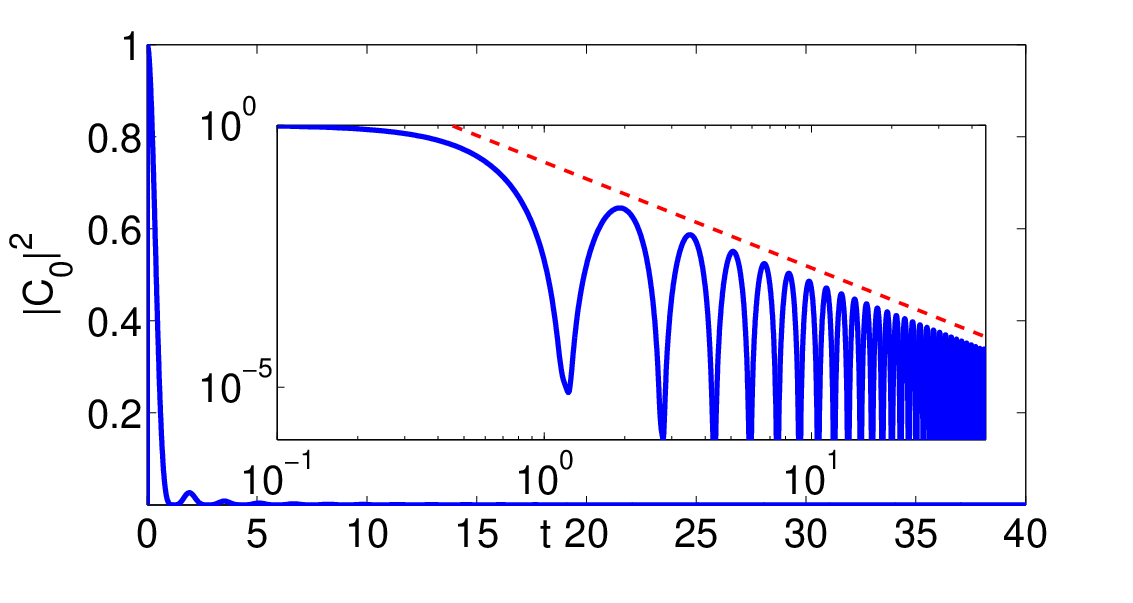
It is also interesting to note that the decay dynamics follows a very typical pattern similar to the one shown in the upper panel of Fig. 2. The corresponding log-log plot inset indicates that the central site amplitude decreases according to a power law (in terms of its envelope). Essentially, in accordance with our arguments in Sec. II (recall (III) and the relevant discussion above), once the linear regime sets in the nonlinearity is irrelevant and plays a negligible role in the ensuing dynamics, which is governed by the linear decay. On the other hand, as illustrated in the right panel, past the actual critical point , only a transient decay is observed, past which the amplitude settles to a constant value and to the corresponding defect mode.
 |
 |
The quantity in the case of D and D-lattices is shown in the upper and lower panel of Fig. 3, respectively for the case of the power nonlinearity. The numerical critical values when , in the D, D and D cases, are given in table 1. Remarkably, we observe the considerable increase of the critical values with respect to the dimension, while as a function of the nonlinearity exponent , the real critical point preserves its monotonicity property as in the D-case. Both properties have been rigorously predicted for the value for the creation of stationary states by Corollaries IV.1.A and IV.2.1-2. The monotonicity property was also expected for the dynamical problem, at least in the case of the D-lattice, from our asymptotic linearization arguments in Sec. II-see eq. 3.28. The last column of table 1, justifies that the theoretical value is also of reasonable quantitative value as an approximation to the lower bound of for the dynamical self-trapping transition.
Fig. 4 summarizes the plots of against for the saturable nonlinearity. We observe again the considerable increase of the critical values with respect to the dimension of the lattice, as predicted by Corollary IV.2.1. Also, table 2 highlights that the theoretical threshold for the creation of stationary states is again of reasonable quantitative value as a prediction of the lower bound of for the dynamical self-trapping transition.
Figs. 5 and 6 show typical examples of the decay and self-trapping dynamics in the D and D-lattices, respectively. The examples concern the power nonlinearity. In the examples of the weak nonlinearity regime shown in the upper panels of Figs. 5 and 6, we observe a drastic decrease of the time interval for the transient, non-vanishing behavior, and an almost instantaneous decay. This effect is even stronger in the D-case. On the other hand, in the examples of the strong nonlinearity regime shown in the bottom panels, we observe a decrease of the time interval of the transient behavior before the convergence of the amplitude to its constant value, and to the corresponding defect mode. This behavior combined with the increase of the critical points with respect to dimension, suggests the following: for higher dimensional lattices, stronger nonlinearity effects should be considered for self-trapping and localization of energy, due to a potential energy dispersion and delocalization associated with the higher dimensional set-ups.
Similar features were observed in the case of saturable nonlinearity. A typical example is shown in Fig. 7. In particular, in the bottom panel concerning the strong nonlinearity regime, we observe a rapid convergence of to the stationary mode, similarly to what is shown in the D example for the cubic power nonlinearity (shown in the bottom panel of Fig. 6).
We finally remark on the rate of decay of the central site amplitude in the D and D-cases. The corresponding log-log plot insets in Figures 5, 6 and 7, indicate that the central site amplitude decreases according to a power law (in terms of its envelope), for , in the case of the power nonlinearity. Thus for all , the numerical results suggest that . This could be reasonable by the linear approximation, where . Having in mind that for large, the linear approximation clearly suggests that . Such a power law could associate the diagnostics (1.1) and (1.6), in the sense that such a power law decay implies that .
| 3.2 | 5.48 | 7.05 | 2 | |
| 6.8 | 9.2 | 11.2 | 4 | |
| 9.2 | 12.0 | 14.2 | 8 |
| 4.4 | 4 | |
| 10.9 | 8 | |
| 15.4 | 12 |
 |
 |
 |
 |
 |
 |
 |
VI Conclusions and Future Challenges
In the present paper, we have revisited the widely relevant theme of a single nonlinear defect embedded in an otherwise linear lattice. We have addressed this problem from an up to now missing rigorous dynamical perspective enabling the characterization of a weak nonlinearity regime, via a suitable contraction mapping argument. This enabled us (for different nonlinearity strengths and for different nonlinearity forms –power law and saturable–) to come up with a proof of the fact that for a sufficiently weak nonlinearity, at least in the D-case. The technical restriction to dimension is imposed by the divergent nature of the integrals of the kernel of the associated integral equation, in lower dimensions .
On the other hand, motivated by numerical observations that in the self-trapping regime the dynamics suggest convergence to a stationary mode, we have considered the existence of minimal values of the nonlinearity strength for the creation of such modes. Our purely variational approach, enabled the construction of such modes as minimizers of the Hamiltonian energy, suggesting their dynamical stability as ground states. Their existence was proved under the assumption that the nonlinearity strength satisfies explicit lower bounds, relevant to those which may be obtained by local bifurcation theory, and in particular, bifurcation from the principal eigenvalue. Interestingly enough, the lower bounds for the creation of stationary states share the main qualitative features of the actual critical values for self-trapping observed in the dynamical problem, namely: the increase of the critical value as dimension increases, and the increase of the critical value as the nonlinearity exponent of the power nonlinearity also increases. The former suggests that stronger nonlinear effects are needed to compensate energy dispersion in higher-dimensional lattices. Moreover, comparing the critical values for the cubic power nonlinearity against the critical values for the saturable one, it was found that higher amplitudes are needed in the saturable case for self-trapping, than in the cubic case. This ordering of critical values can be explained by the sub-linear (e.g. closer to the linear limit) nature of the saturable nonlinearity. Notably, this effect is also suggested by the variational bounds of critical points for the creation of stationary modes.
 |
 |
Naturally, there are numerous open questions that are still in need of rigorous analysis. An important one concerns the extension of the rigorous dynamical arguments in the lower dimensional cases (dimensions of the lattice ). Another important question concerns an improved estimation of the true threshold separating the weakly nonlinear (dispersing) from the self-trapping regime. However, clearly the techniques to address the latter issue should be of a fundamentally different kind than the ones used herein, and could be possibly based on analytical bifurcation theory for nonlinear integral equations. On a related note, generalization of either the former (contraction mapping, possibly combined with invariance arguments for the integral map in suitable function spaces) or the latter (analytical bifurcation theory) considerations to multi-dimensional or multi-defect settings would also be of particular interest. However, there remain intriguing questions even at the computational level and even in the one-dimensional setting. For instance, a separate theme of interest for future study would be to examine the asymptotic profile to which the self-trapping dynamics results and the “selection principle” of this state, among the family of possible stationary states with different norms/energies. Similar investigations have been numerically initiated also in the case of the fully nonlinear DNLS lattice in [28]. These themes are presently under consideration and will be reported in future publications.
Acknowledgments. PGK gratefully acknowledges support from the NSF under grants DMS-1312856 and CMMI-1000337, as well as from the AFOSR under grant FA950-12-1-0332, the Binational Science Foundation under grant 2010239, from the Alexander von Humboldt Foundation and the FP7, Marie Curie Actions, People, International Research Staff Exchange Scheme (IRSES-606096). He also acknowledges the hospitality of the IMA of the University of Minnesota during the final stages of this work. MIM acknowledges support from Fondo Nacional de Ciencia y Tecnología (Grant 1120123), Programa Iniciativa Científica Milenio (Grant P10-030-F) and Programa de Financiamiento Basal (Grant FB0824).
VII Appendix
VII.1 Eigenvalues of the Dirichlet Discrete Laplacian
In this part of the complementary section we provide for completeness, some information on the eigenvalue problem for the discrete Laplacian. For , we consider the problem
| (7.1) |
considered in the -dimensional cube of with edges of length ,
The discrete eigenfunctions on are denoted by
The interior of the cube is given by
and (7.1) is supplemented with Dirichlet boundary conditions
| (7.2) |
Thus, the finite dimensional problem (7.1)–(7.2) is formulated in the finite dimensional subspace of the sequence space ,
| (7.3) |
where .
When , the space becomes a real Hilbert space, , if endowed with the real inner product
In the above real Hilbert space which will be still denoted for simplicity, by , the operator is self-adjoint. Moreover, the eigenvalues of the discrete eigenvalue problem (7.1)-(7.2) in the finite dimensional space , coincide with those of its real counterpart (e.g. for ), and are the following:
while its principal eigenvalue is
According to the variational characterization of the eigenvalues of the discrete Laplacian in the finite dimensional subspaces , , can be characterized as
Then, (VII.1) implies the inequality
| (7.7) | |||||
VII.2 Algebra with special functions
The integral in (4.8), is of the form
| (7.8) |
To calculate this integral, we recall first the relation of the Legendre function of the 1st kind with the hypergeometric function , for [20, Sec. 8.82-8.83, eq. (6)],
| (7.9) | |||||
Setting and in (7.9) we get that
| (7.10) |
We recall further, that the right hand side of (7.10) is associated the complete elliptic integral of the 1st kind, with modulus , [20, Sec. 8.113, eq. (1)],
| (7.11) | |||||
Besides, from [20, Sec. 6.672, eq. (5)],
| (7.12) | |||||
where is the Legendre function of the 2nd kind. Setting , in (7.12), we get that
| (7.13) | |||||
Note that both functions and are related for , with the formula [20, Sec. 6.672, eq. (5)],
| (7.14) |
Setting and , for in (7.14), we recover
| (7.15) |
Combining the branch of (7.13) for the case , with (7.15), we find that
| (7.16) | |||||
Hence, from (7.10), (7.11) and (7.16) we conclude in
| (7.17) | |||||
References
- [1]
G.P. Tsironis, M.I. Molina and D. Hennig,
Phys. Rev. E 50, 2365 (1994).
- [2]
M. I. Molina, Mod. Phys. Lett. B 17, 111 (2003).
- [3]
M.I. Molina, H. Bahlouli
Phys. Lett. A 284, 87 (2002).
- [4]
K. Hizanidis, Y. Kominis and N.K. Efremidis,
Opt. Express 16, 18296 (2008).
- [5] F. Delyon, I.-E. Lévy, B. Souillard, Phys. Rev. Lett. 57, 2010 (1986).
- [6] Y. Wan and C.M. Soukoulis, Phys. Rev. A 41, 800 (1990).
- [7] M.I. Molina and G.P. Tsironis, Phys. Rev. B 47, 15330 (1993).
- [8] D. Chen, M.I. Molina, G.P. Tsironis, J. Phys.: Condens. Matter 5, 8689 (1993).
- [9] G. P. Tsironis, M. I. Molina and D. Hennig, Phys. Rev. B 50, 2365 (1994).
- [10] V. A. Brazhnyi and B. A. Malomed, Phys. Rev. A 83, 053844 (2011).
- [11] B. A. Malomed, E. Ding, K. W. Chow and S. K. Lai, Phys. Rev. E 86, 036608 (2012).
- [12] J. D’Ambroise, P.G. Kevrekidis and S. Lepri, Chaos 23, 023109 (2013).
- [13] J. D’Ambroise, P.G. Kevrekidis, S. Lepri, J. Phys. A 45, 444012 (2012).
- [14] X. Zhang, J. Chai, J. Huang, Z. Chen, Y. Li and B.A. Malomed, Opt. Express 22, 13927 (2014).
- [15] P.G. Kevrekidis, The discrete nonlinear Schrödinger equation: mathematical analysis, numerical computations and physical perspectives, Springer-Verlag (Heidelberg, 2009).
- [16] P. G. Kevrekidis, H. Susanto and Z. Chen, Phys. Rev. E 74, 066606 (2006).
- [17] R. Adams. Sobolev Spaces. Academic Press (New York, 1975).
- [18] J. Ginibre and G. Velo. Physica D, 95 191 (1996).
- [19] M. Abramowitz and I. A. Stegun. Handbook of Mathematical Functions With Formulas, Graphs and Mathematical Tables. U. S. National Bureau of Standards, Mathematical Series 55, 1972.
- [20] I. S. Gradshteyn and I. M. Ryzhik. Table of Integrals, Series, and Products, Academic Press (New York, 1996).
- [21] E. Zeidler. Nonlinear Functional Analysis and its Applications I: Fixed Point theorems. Springer-Verlag, 1986.
- [22] N.I. Karachalios, B. Sánchez-Rey, P.G. Kevrekidis and J. Cuevas, J. Nonlinear Sci. 23, no. 2, 205 (2013).
- [23] J. Cuevas, N. I. Karachalios, F. Palmero. Appl. Anal. 89, 1351 (2010).
- [24] J. Cuevas, J. C. Eilbeck, N. I. Karachalios. Dyn. Partial Differ. Equ. 5, 69 (2008).
- [25] J. Cuevas, J. C. Eilbeck, N. I. Karachalios. Discrete Contin. Dyn. Syst. A 21, 445 (2008).
- [26] M. Crandall and P. Rabinowitz. J. Functional Analysis 8, 321 (1970).
- [27] V. Achilleos, G. Theocharis, P. G. Kevrekidis, N. I. Karachalios F. Diakonos and d. J. Frantzeskakis. J. Math. Phys. 52, 092701 (2011).
- [28] P.G. Kevrekidis, J.A. Espinola-Rocha, Y. Drossinos and A. Stefanov, Phys. Lett. A 372, 2247 (2008).