Nonequilibrium transport through magnetic vibrating molecules

For $\lambda=0$, the model reduces to the ordinary impurity Anderson model. and its main properties are well known.[48] In particular, in the Kondo regime $\epsilon_{F}-E_{d}\gg V_{K}$ where $\epsilon_{F}$ is the Fermi energy and $K$ denotes $k,\nu$, the characteristic low-energy scale is given by the Kondo temperature $T_{K}\sim\exp\left[-1/(\rho J)\right]$, where $\rho$ is the spectral density of the conduction states for given spin, and for $U\longrightarrow\infty$ (which corresponds to our NCA calculations) $J=2|V_{K}|^{2}/(\epsilon_{F}-E_{d})$ for constant $V_{K}$. The half width at half maximum of the peak near the Fermi energy in the spectral density $\rho(\omega)$ is proportional to $T_{K}$, as well as the corresponding widths of the peaks of the conductance $G(T,V_{b})=dI/dV_{b}$ as a function of temperature $T$ and bias voltage $V_{b}$ near $T=V_{b}=0$ ($I$ is the current).[49] Any of these half widths might be used as a definition of $T_{K}$. Here we use that of $\rho(\omega)$.

If the electrons could be decoupled from the phonons in some approximation, one might expect that an effective purely electronic model $H_{\mathrm{eff}}$ of the form of the ordinary impurity Anderson model, but with renormalized parameters, $\tilde{E_{d}}$, $\tilde{V}_{K}$ describes the electronic motion, leading to a renormalized Kondo temperature $T_{K}\sim\exp\left[-1/(2\rho|\tilde{V}_{K}|^{2}/(\epsilon_{F}-\tilde{E_{d}}))\right]$. How $T_{K}$ varies with $\lambda$ will be discussed in Section IV.1. For this discussion, it is necessary to define $\tilde{E_{d}}$ in some way. In the rest of this Section we discuss this definition and some limits of the model.

The model given by Eq. (1) can be solved exactly for $V_{k}^{\nu}=V_{K}=0$. In this case, the total number of electrons in the molecule $n_{d}$ is a good quantum number and the electron-phonon interaction $\lambda$ can be eliminated by a simple shift in the phonon operator $\beta^{\dagger}=a^{\dagger}+\hat{c}$, where $\hat{c}$ is an operator that depends on $n_{d}$. This simply reflects the fact that the equilibrium position of the normal-mode coordinate depends on the occupation. It is easy to see that for each $n_{d}$, one has

where $\Delta E$ is the energy gain due to the electron-phonon interaction. Then, for $V_{k}^{\nu}=0$, the Hamiltonian takes the form

where the subscript 0 reminds us that (for the moment) $V_{K}=0$ and the renormalized level energy and Coulomb repulsion are

For very large $\omega_{0}$, the last term of Eq. (3) can be neglected and $H_{0}$ reduces to a purely electronic model with effective parameters. In this antiadiabatic approximation,[50] when one includes the hybridization term, it becomes exponentially reduced, due to the fact that it mixes states with different $n_{d}$, and the scalar product of the phonon wave functions with different equilibrium positions leads to a factor $\tilde{V}_{K}/V_{K}=\exp[-(\lambda/\omega_{0})^{2}/2]$.[28] Thus, the effective Hamiltonian for $\omega_{0}\longrightarrow\infty$ becomes

with $\tilde{E_{d}}=\tilde{E_{d}^{0}}$.

The limit $\omega_{0}\longrightarrow\infty$ is however not realistic. In the general case, the electron-phonon interaction can also be eliminated using a Lang-Firsov unitary transformation.[51, 52] The price to pay is that $\tilde{V}_{K}$ includes exponentials of phonon operators which are usually treated in a decoupling approximation, which as in the antiadiabatic limit, usually leads to an exponential dependence of $T_{K}$ on $\lambda$ for fixed $\tilde{E_{d}^{0}}$, which is not found in more elaborate treatments.[23, 29, 31]

In any case, if the antiadiabatic limit, or a decoupling approximation leading to a purely electronic Hamiltonian $H_{\mathrm{eff}}$ has to be abandoned, one might ask if the renormalized level energy $\tilde{E_{d}}$ is still given by $\tilde{E_{d}^{0}}$ [first Eq. (4)] in a more elaborate treatment. This equation comes as a result of optimizing the energy neglecting the hybridization, leading to a shift given by the first Eq. (2) in the equilibrium position of the oscillator. One expects that for large hybridization, a smaller shift giving rise to a smaller gain of elastic energy but a larger gain in hybridization energy is more convenient. Here we define

where $|g\rangle$ is the ground state and $P_{n}$ is a projector on the subspace with $n_{d}=n$. We have estimated $\tilde{E_{d}}$ using a simple variational approximation, where $\hat{c}$ is replaced by a constant $c$ obtained minimizing the ground-sate energy. The details are given in appendix A. The first Eq. (18) shows that the phonon shift has in fact smaller magnitude than $\lambda/\omega_{0}$ and Eq. (20) gives a smaller shift of $\tilde{E_{d}}$ than the corresponding one Eq. (4) for zero hybridization. However, the variational approach is too simple and we do not pretend this result to be quantitatively valid. Qualitative aspects will be discussed in Section IV.2

In order to test the NCA for the phonons, we represent in Fig. 2 the spectral density of the physical fermion $\rho_{d\sigma}(\omega)$ in the particular case of zero hybridization $V_{k}^{\nu}=0$, for several values of the electron-phonon interaction $\lambda$, and compare it with the exact result.[36] We used a logarithmic scale to render visible the second replica of the main peak. For $V_{k}^{\nu}=0$, $n_{d}$ is a good quantum number and the problem can be solved exactly shifting the phonon operators depending on the occupation [see Eq. (3)]. This shift is not explicit in the NCA and it is not obvious that the correct physics is reproduced by the NCA for large $\lambda$. For $\tilde{E_{d}}<\epsilon_{F}=0$, and temperature $T=0$, one has $n_{d}=1$. Thus, for infinite $U$ as we assume, electrons can only be destroyed at the dot and from the Lehman representation of the Green’s function,[52] it is clear that the spectral density has components only at negative frequencies. The main peak should be at $\omega=\tilde{E_{d}}$, where for $V_{k}^{\nu}=0$, $\tilde{E_{d}}=\tilde{E_{d}^{0}}=E_{d}-\lambda^{2}/\omega_{0}$, and its intensity is proportional to the square of the overlap between the ground state of the phonon wave functions for $n_{d}=0$ (vacuum of phonon operator $a$) and $n_{d}=1$ (vacuum of phonon operator $\beta$). There are more peaks shifted at lower energies by $n\omega_{0}$ with amplitude reduced by the overlap between the phonon ground state $|0_{\beta}\rangle$ for displaced phonons and the state $|n_{a}\rangle$ with $n$ undisplaced phonons. As seen in the figure, the NCA reproduces very well the intensity and position of the main peak. For large $\lambda$, the position of this peak is slightly displaced from $\tilde{E_{d}}$. The shift $\lambda^{2}/\omega_{0}$ is overestimated by about 5% for $\lambda=0.5\omega_{0}$. The replicas are shifted to lower energies by the NCA, and their intensities are underestimated, but the NCA results remain semiquantitatively valid.

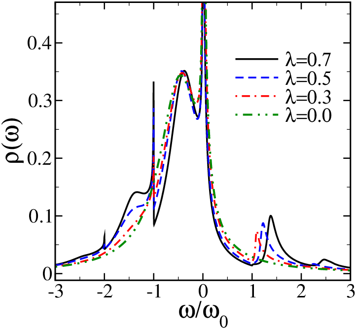
From now on, we discuss the results for $V_{K}\neq 0$. In Fig. 3 we show the spectral density of the physical fermion $\rho_{d\sigma}(\omega)$ for several values of the electron-phonon interaction $\lambda$. This figure has the same parameters as Fig. 6 of Ref. 29. The case $\lambda=0$ is known, and one can see the usual narrow Kondo peak at the Fermi energy $\epsilon_{F}=0$, and the broad charge-transfer peak near the energy $\tilde{E_{d}^{0}}$. Both peaks clearly narrow with increasing $\lambda$. In addition, for $\lambda\neq 0$, both peaks have replicas with lower intensity shifted to negative frequencies by the phonon energy $\omega_{0}$. The replicas of the charge-transfer peak can just be interpreted as a broadening of the peaks shown in Fig. 2 as a consequence of the hybridization. In agreement with the EOM results of Ref. 29, we do not see replicas of the charge-transfer peak at positive frequencies. This is expected, since this peak is due to annihiliation of the occupied molecular state and the spectral weight of this peak at positive frequencies (creation of this state) is very small for $U\rightarrow\infty$.

The replicas of the Kondo peak are more subtle. The Kondo peak is due to small charge fluctuations near the Fermi level and has contributions at both positive (creation of an electron at the localized level $d^{\dagger}_{\sigma}$) and negative (annihilation) frequencies. From the Lehman representation of the Green’s function,[52] the spectral density at $\omega=-\omega_{0}^{\ast}$, with $\omega_{0}^{\ast}$ near $\omega_{0}$, at zero temperature, is given by

where the states here are eigenstates of the complete Hamiltonian with electrons and phonons. $|g\rangle$ is the ground state, and $|e\rangle$ are excited states with excitation energy $\epsilon_{e}$ (the difference between the energy of the state $|e\rangle$ and the ground state energy $E_{g}$).

We denote as $|e^{0}_{n}\rangle$, the eigenstates for $\lambda=0$ with $n$ phonons added to the vacuum of the uncharged system ($|0_{a}\rangle$). $|g^{0}_{0}\rangle$ is the ground state for $\lambda=0$ (see Fig. 4). Note that the electronic part of these states is independent of $n$, the phonon part of the energy is just $n\omega_{0}$ and $\langle e^{0}_{n}|d_{\sigma}|g^{0}_{n}\rangle$ is independent of $n$. We also call $|e^{K}_{n}\rangle$ the states $|e^{0}_{n}\rangle$ with very small electronic excitation energy and $n$ phonons, which for $n=0$ are responsible for the Kondo peak when $\lambda=0$. For finite $\lambda$, the electron-phonon interaction mixes the states $|e^{0}_{n}\rangle$ and $|g^{0}_{n}\rangle$ (which are no longer eigenstates) with those with $n\pm 1$ phonons. In particular, the ground state $|g\rangle$ which for $\lambda=0$ is $|g^{0}_{0}\rangle$ acquires some component of $|g^{0}_{1}\rangle$ (and smaller ones of $|g^{0}_{n}\rangle$). In turn, the states $|e\rangle$, which for $\lambda=0$ are $|e^{K}_{1}\rangle$ (with energy near $E_{g}+\omega_{0}$) obtain some amount of $|e^{K}_{0}\rangle$ after turning on $\lambda$. These new components of the eigenstates lead to contributions to the matrix elements entering Eq. (14), which are similar to those of the Kondo peak and increase linearly with $\lambda/\omega_{0}$ for small $\lambda$. In addition, the states $|e^{0}_{0}\rangle$ with energy near $E_{g}+\omega_{0}$ which have a large contribution to Eq. (14) for $\lambda=0$ are expected to have a large mixing with $|e^{K}_{1}\rangle$ for finite $\lambda$ because the have nearly the same energy. Both effects contribute to “translate” the electronic structure of the Kondo effect contained in $|e^{K}_{n}\rangle$ to the spectral density at $\omega\approx-n\omega_{0}$.

An analogous reasoning can be followed for $\rho_{d\sigma}(\omega_{0}^{\ast})$ (positive frequencies) changing $d_{\sigma}$ by $d_{\sigma}^{\dagger}$ in Eq. (14). For $\omega>\omega_{0}$, we obtain broad structures centered slightly below $\omega=n\omega_{0}+\lambda^{2}/\omega_{0}$, with $n$ integer. An observation of the first one ($n=1$), indicates a small jump with increase in intensity at $\omega=\omega_{0}$ and a smooth evolution of the intensity with increasing $\omega$. While we do not have reached a complete understanding, several pieces of evidence (given below) indicate that this peak is a broadened replica of the Kondo peak. The shift in position with respect to $\omega_{0}$ seems to be related with a loss of the energy gain $\Delta E$ [see Eq. (2)] in most of the excited states involved in the spectral decomposition of $d^{\dagger}_{\sigma}|g>$. The broadening of the peak seems to be related in the uncertainty in the equilibrium position of the oscillator since $n_{d}$ is not well defined. The position of this peak does not change with $E_{d}$ as it might be expected for a feature related with the charge transfer peak. This is shown in Fig. 5. From the figure, one also sees that as $E_{d}$ decreases, the weight of this peak decreases. This is what is expected for a Kondo peak, since its total weight is proportional to $T_{K}$, which decreases with decreasing $E_{d}$ (see Section II.1).

As discussed in more detail below, the evolution with temperature of the peak (see Fig. 6) also suggests that it is related with the Kondo one, which in contrast to the charge-transfer peak, decreases in intensity as the temperature is increased.

The replica of the Kondo peak at $\omega=-\omega_{0}$ is quite sharp. This is due to the fact explained in the previous section, that the phonon spectral density is not renormalized within the NCA. Therefore, the softening and damping of the phonon mode due to its interaction with the electrons, is absent. The phonon damping would broaden the replicas of the Kondo effect, in a more realistic description. However, it remains unclear to us, why the replicas at negative frequencies are quite sharp, while those at positive frequency are broadened by some energy related with $\Delta E$ [see Eq. (2)]. Further studies with a technique that allows finite $U$ might shed light on this issue.

The results displayed in Fig. 3 are qualitatively similar to those obtained previously using equations of motion [Fig. 6 of Ref. 29], but there are quantitative differences. The replica of the Kondo peak at $\omega$ near $\omega_{0}$, is sharper in their work and located exactly at $\omega=\omega_{0}$. Instead, the replica of the Kondo peak near $-\omega_{0}$ seems absent in Ref. 29 and for larger $\lambda$, the spectral density seems to approach vanishing values near $\omega=\pm\omega_{0}$.

In Fig. 6 we show the evolution of the spectral density $\rho_{d\sigma}(\omega)$ with temperature. As it is known for the case with $\lambda=0$, there is a strong temperature dependence of the peak at the Fermi energy (the Kondo peak) at temperatures of the order of the Kondo temperature $T_{K}$. We define $T_{K}$ as the half width at half maximum of the Kondo peak at zero temperature. We observe a similar strong dependence of the satellite peaks near $\omega=\pm\omega_{0}$ suggesting that these peaks are replicas of the low-energy Kondo screening of the local magnetic moment combined with the effect of one virtual phonon. For example, while the intensity of the charge transfer peak near $\tilde{E_{d}}$ or its replica at $\tilde{E_{d}}-\omega_{0}$ hardly changes for temperatures of the order of $T_{K}$, the other peaks strongly lose intensity (for $\omega\sim 1.34\omega_{0}$) or disappear (for $\omega\sim 0,-\omega_{0},-2\omega_{0}$) for $T=0.1>T_{K}\approx 0.01\omega_{0}$. In any case, the fact that a broad structure near $1.35\sim\omega_{0}$ remains at that temperature is rather unexpected.

In presence of the electron-phonon interaction $\lambda$, for a fixed renormalized localized level $\tilde{E_{d}}$, $T_{K}$ is expected to decrease with increasing $\lambda$, due to the renormalization of the hybridization $V$. However, an exponential decrease (as predicted using simple decouplings of electrons and phonons) is not expected.[23, 29]

The inset of Fig. 7 displays our results for $T_{K}$ as function of $\lambda$ for fixed $\tilde{E_{d}^{0}}$. As in Ref. 29 we obtain a moderate decrease of $T_{K}$ as the electron-phonon interaction $\lambda$ increases. However, in our case we find a plateau between $0.6<\lambda/\omega_{0}<0.7$, which at fist sight seems surprising. We ascribe this effect to the fact that while $\tilde{E_{d}^{0}}$ is constant, the real effective localized level $\tilde{E_{d}}$ increases with $\lambda$ in this interval and there is a compensation of this effect (which tends to increase $T_{K}$) with the monotonic decrease of $T_{K}$ with $\lambda$ for fixed $\tilde{E_{d}}$. Below we provide several arguments and calculations to support our conclusion. One of them is that the maximum of the charge transfer peak near $\omega\approx-0.4\omega_{0}$ in Fig. 7 moves to the right as lambda decreases. Note that the usual upward shift in the renormalized localized level $(\Delta/\pi){\rm ln}(D/\Delta)$ calculated with poor man’s scaling [58] leads to a shift in the opposite direction because the effective resonant level width decreases.

In Fig. 8 we show $\Delta E_{d}=\tilde{E_{d}}-\tilde{E_{d}^{0}}$ as a function of $\lambda$ with $E_{d}$ calculated variationally as discussed in Section II.1. With respect of the parameters of Fig. 7, we have multiplied $\Delta$ by a factor 2 because it leads approximately to the correct occupancy of the localized level when compared with NRG results [59]. Although the variational calculation can provide only qualitative results, one can see that it predicts the steepest increase of $\Delta E_{d}$ with $\lambda$ near $\lambda/\omega_{0}=0.5$ and a saturation for larger $\lambda$, which is consistent with the existence of the plateau in Fig. 7. Further evidence for a shift in $\Delta E_{d}$ as a cause of this plateau is provided by the dependence of the occupancy of the localized level with $\lambda$ (calculated with NCA). This is displayed in Fig. 9 and shows a behavior which is reminiscent of that of $\Delta E_{d}$ with a maximum near $\lambda/\omega_{0}=0.5$.

As a final analysis of this situation, we have repeated several NCA calculations for each value of the electron-phonon interaction $\lambda$, shifting the bare level $E_{d}$ in such a way that the maximum of the charge-transfer peak (near $\omega\approx-0.4\omega_{0}$ in Fig. 7) lies at the same position as for $\lambda=0$, with an error smaller than a fraction of $T_{K}$. This procedure is very time consuming, but since the NCA is much superior than the variational calculation, it ensures that we are working at constant effective renormalized localized level $\tilde{E_{d}}$ with reasonable accuracy.

The results are displayed in Fig. 10. In contrast to Fig. 7 one can see that the position of the charge-transfer peak remains constant, while it narrows as $\lambda$ increases. Now we obtain a nice monotonic decrease of $T_{K}$ with $\lambda$ as expected. Also the occupancy of the localized level (not shown) has now a monotonic increase with $\lambda$ from 0.79 for $\lambda=0$ to 0.87 for $\lambda=0.87\omega_{0}$.

A quantitative analysis of the narrowing of the charge-transfer peak is complicated by the presence of the side Kondo peaks and is beyond the scope of the present work. In any case, it seems that the NCA does not give an exponential reduction of this width with increasing electron-phonon interaction $\lambda$ for fixed renormalized localized level $\tilde{E_{d}}$. Although an exponential renormalization factor is a common feature of strongly coupled electron-phonon couplings, as stressed by Hewson and Mayer, the exponential reduction does not in general occur in the strong-coupling regime of the model, but only in a certain parameter regime.[23]

In Fig. 11 the evolution of $\rho_{d\sigma}(\omega)$ with applied bias voltage $V_{b}$ is displayed. We see that in addition of the known splitting of the Kondo peak with $V_{b}$,[39, 40] also the replica of the Kondo peak near $\omega=-\omega_{0}$ splits, a fact which again supports the notion that this satellite peak is related with the Kondo peak at the Fermi energy. For $\omega\approx 1.35\omega_{0}$, a splitting also takes place, but only for bias voltage large enough so that $eV_{b}$ overcomes the intrinsic width of this feature. The inset shows that the onset of this peak at $\omega=\omega_{0}$, is also split by the bias voltage, and the splitting is clearly visible already for small bias voltages, of the order of a few times $T_{K}/e$.

In Fig. 12 we display the conductance $G=dI/dV_{b}$, where $I$ is the current as a function of a applied bias voltage $V_{b}$ for a temperature slightly above the Kondo temperature and several values of the electron-phonon interaction. In addition to the Kondo peak at $V_{b}=0$, and the charge-transfer peak near $V_{b}=\pm\tilde{E_{d}}$ replicas of the Kondo peak with smaller intensity appear for $eV_{b}=\pm 2\omega_{0}$ reflecting the inelastic processes in which a phonon is created or destroyed. Since the curve is symmetric with respect to a change of sign of the bias voltage [$G(-V_{b})=G(V_{b})$] only positive $V_{b}$ are shown. In general, further peaks at $eV_{b}=\pm 2n\omega_{0}$ with $n>1$ are expected, as observed experimentally.[17] These are difficult to capture within NCA due to the limitations of the numerical procedure at very low temperatures.

For experiments of transport through molecules, the couplings to the leads $\Gamma_{\nu}$ are very asymmetric in general. In Fig. 13 we show the nonequilibrium conductance for a case in which $\Gamma_{L}=30\Gamma_{R}$ (typical of experiments with C₆₀ quantum dots [12]), keeping $\Gamma_{R}+\Gamma_{L}=2\Delta$, and the voltage drop is inversely proportional to the corresponding $\Gamma_{\nu}$: $\mu_{L}=(1/31)V_{b}$, $\mu_{R}=(-30/31)V_{b}$. In this case, the spectral density at the molecule for finite bias voltage $V_{b}$ is similar to that in which the dot is at equilibrium with the lead for which the coupling is the largest, and is not strongly modified by $V_{b}$. Since most of voltage drop falls between the system and the other lead, the situation is similar to that in scanning tunneling microscopy (STM), in which the spectral density is little affected by the less coupled lead (or STM tip) and the spectral density is reflected in the differential conductance $G(V_{b})$.[57] Therefore, the resulting conductance is qualitatively similar to the spectral density as a function of frequency, shown before in Fig. 6.

References

- [1] A. Nitzan and M. A. Ratner, Science 300, 1384 (2003).
- [2] L. Venkataraman, J. E. Klare, C. Nuckolls, M. S. Hybertsen, and M. L. Steigerwald, Nature (London) 442, 904 (2006).
- [3] M. Galperin, M. A. Ratner, A. Nitzan, and A. Troisi, Science 319, 1056 (2008).
- [4] S. J. van der Molen and P. Liljeroth, J. Phys. Condens. Matter 22, 133001 (2010).
- [5] J. C. Cuevas and E. Scheer, Molecular Electronics: An Introduction to Theory and Experiment (World Scientific, Singapore, 2010).
- [6] J. Park, A. N. Pasupathy, J. I. Goldsmith, C. Chang, Y. Yaish, J. R. Petta, M. Rinkoski, J. P. Sethna, H. D. Abruña, P. L. McEuen, and D. C. Ralph, Nature (London) 417, 722 (2002).
- [7] W. Lian, M. P. Shores, M. Bockrath, J. R. Long, and H. Park, Nature (London) 417, 725 (2002).
- [8] E. A. Osorio, K. O’Neill, M. Wegewijs, N. Stuhr-Hansen ,J. Paaske , T. Bjornholm, and H. S. J. van der Zant, Nano Lett. 7, 3336 (2007).
- [9] I. Fernández-Torrente, K. J. Franke, and J. I. Pascual, Phys. Rev. Lett. 101, 217203 (2008).
- [10] N. Roch, S. Florens, V. Bouchiat, W. Wernsdorfer, and F. Balestro, Nature 453, 633 (2008).
- [11] J. J. Parks, A. R. Champagne, T. A. Costi, W. W. Shum, A. N. Pasupathy, E. Neuscamman, S. Flores-Torres, P. S. Cornaglia, A. A. Aligia, C. A. Balseiro, G. K.-L. Chan, H. D. Abruña, and D. C. Ralph, Science 328, 1370 (2010).
- [12] S. Florens, A, Freyn, N. Roch, W. Wernsdorfer, F. Balestro, P. Roura-Bas and A. A. Aligia, J. Phys. Condens. Matter 23, 243202 (2011).
- [13] D. E. Logan, C. J. Wright, and M. R. Galpin, Phys. Rev. B 80, 125117 (2009).
- [14] P. Roura-Bas and A. A. Aligia, Phys. Rev. B 80, 035308 (2009).
- [15] P. Roura-Bas and A. A. Aligia, J. Phys. Cond. Matt. 22, 025602 (2010).
- [16] H. Park, J. Park, A. K. L. Lim, E. H. Anderson, A. P. Alivisatos, and P. L. McEuen, Nature (London) 407, 57 (2000).
- [17] N. B. Zhitenev, H. Meng, and Z. Bao, Phys. Rev. Lett. 88, 226801 (2002).
- [18] M. Berthe, A. Urbieta, L. Perdigao, B. Grandidier, D. Deresmes, C. Delerue, D. Stievenard, R. Rurali, N. Lorente, L. Magaud, and P. Ordejon, Phys. Rev. Lett. 97, 206801 (2006).
- [19] M. Galperin, M. A. Ratner, and A. Nitzan, J. Phys.: Condens. Matter 19, 103201 (2007).
- [20] S. Ballmann, R. Härtle, P. B. Coto, M. Elbing, M. Mayor, M. R. Bryce, M. Thoss, and H. B. Weber, Phys. Rev. Lett. 109, 056801 (2012).
- [21] L. H. Yu, Z. K. Keane, J. W. Ciszek, L. Cheng, J. M. Tour, T. Baruah, M. R. Pederson, and D. Natelson, Phys. Rev. Lett. 95, 256803 (2005).
- [22] P. S. Cornaglia, G. Usaj, and C. A. Balseiro, Phys. Rev. B 76, 241403(R) (2007).
- [23] A. C. Hewson and D. Meyer, J. Phys.: Condens. Matter 14, 427 (2002).
- [24] P. S. Cornaglia, H. Ness, and D. R. Grempel, Phys. Rev. Lett. 93, 147201 (2004)
- [25] L. Arrachea and M. J. Rozenberg, Phys. Rev. B 72, 041301 (2005).
- [26] M. D. Núñez Regueiro, P. S. Cornaglia, G. Usaj, and C. A. Balseiro, Phys. Rev. B 76, 075425 (2007).
- [27] H-C. Yong, K-H. Yang and G-S. Tian, Commun. Theor. Phys. 48, 1107 (2007).
- [28] A. Martin-Rodero, A. Levy Yeyati, F. Flores, and R. C. Monreal, Phys. Rev. B 78, 235112 (2008).
- [29] R. C. Monreal and A. Martin-Rodero, Phys. Rev. B 79, 115140 (2009).
- [30] J. König, H. Schoeller, and G. Schön, Phys. Rev. Lett. 76, 1715 (1996).
- [31] J. Paaske and K. Flensberg, Phys. Rev. Lett. 94, 176801 (2005).
- [32] M. Galperin, A. Nitzan, and M. A. Ratner, Phys. Rev. B 76, 035301 (2007).
- [33] J. E. Han, Phys. Rev. B 81, 113106 (2010).
- [34] K. H. Yang, Y. P. Wu, and Y. L. Zhao, Europhys. Lett. 89, 37008 (2010).
- [35] A. Goker, J. Phys.: Condens. Matter 23, 125302 (2011).
- [36] R. C. Monreal, F. Flores, and A. Martin-Rodero, Phys. Rev. B 82, 235412 (2010).
- [37] A. Levy Yeyati, A. Martin-Rodero, and F. Flores, Phys. Rev. Lett. 71, 2991 (1993).
- [38] A. A. Aligia, Phys. Rev. B 74, 155125 (2006).
- [39] N. S. Wingreen and Y. Meir, Phys. Rev. B 49, 11040 (1994),
- [40] M. H. Hettler, J. Kroha and S. Hershfield, Phys. Rev. B 58, 5649 (1998).
- [41] T. A. Costi, J. Kroha and P. Wölfle, Phys. Rev. B 53, 1850 (1996).
- [42] P. Roura-Bas, Phys. Rev. B 81, 155327 (2010).
- [43] A. Oguri, J. Phys. Soc. Jpn. 74, 110 (2005).
- [44] A. A. Aligia, J. Phys. Condens. Matter 24, 015306 (2012); references therein; A. A. Aligia, arXiv:1302.4069
- [45] R. V. Roermund, S.-Y. Shiau, and M. Lavagna, Phys. Rev. B 81, 165115 (2010).
- [46] L. Vaugier, A.A. Aligia and A.M. Lobos, Phys. Rev. B 76, 165112 (2007).
- [47] A. Freyn and S. Florens, Phys. Rev. Lett. 107, 017201 (2011).
- [48] A. C. Hewson, in The Kondo Problem to Heavy Fermions (Cambridge, University Press, 1993).
- [49] L. Tosi, P. Roura-Bas, A. M. Llois and A. A. Aligia, Physica B 407, 3263 (2012).
- [50] For nonvanishing in the Kondo regime, the antiadabatic approximation is expected to be valid when , where are defined in Eqs. (13).
- [51] D. C. Langreth, Phys. Rev. B 1, 471 (1970).
- [52] G.D. Mahan, Many Particle Physics (Kluver/Plenum, New York, 2000).
- [53] E.M. Lifshitz and A.L. Pitaevskii, Physical Kinetics (Pergamon, Oxford, 1981).
- [54] Y. Meir and N. S. Wingreen, Phys. Rev. Lett. 68, 2512 (1992).
- [55] A. P. Jauho, N. S. Wingreen, and Y. Meir, Phys. Rev. B 50, 5528 (1994).
- [56] C. M. Varma and Y. Yafet, Phys. Rev. B 13, 2950 (1976).
- [57] A. A. Aligia and A. M. Lobos, J. Phys.: Condens. Matter 17, S1095-S1122 (2005).
- [58] F. D. M. Haldane, Phys. Rev. Lett. 40, 416 (1978).
- [59] P. Roura-Bas, L. Tosi, A. A. Aligia, and P. S. Cornaglia, Phys. Rev. B 68, 165106 (2012).