Unified dispersive approach to real and virtual photon-photon scattering at low energy
Abstract
Previous representations of pion pair production amplitudes by two real photons at low energy, which combine dispersion theoretical constraints with elastic unitarity, chiral symmetry and soft photon constraints are generalized to the case where one photon is virtual. The constructed amplitudes display explicitly the dependence on the phase-shifts, on pion form factors and on pion polarizabilities. They apply both for space-like and time-like virtualities despite the apparent overlap of the left and right-hand cuts, by implementing a definition of resonance exchange amplitudes complying with analyticity and consistent limiting prescriptions for the energy variables. Applications are made to the pion generalized polarizabilies, to vector meson radiative decays, and to the electromagnetic form factor. Finally, an evaluation of the contribution of states in the hadronic vacuum polarization to the muon is given, which should be less model dependent than previous estimates.
1 Introduction
A precise knowledge of the amplitudes for producing a small number of pions from a pair of real or virtual photons is needed for a reliable evaluation of the hadronic light-by-light contribution to the muon . Recently, the contribution which involves the intermediate states was evaluated to NNLO in the chiral expansion [1]. The convergence of the chiral expansion is somewhat slowed down, in this context, by the strong attraction of the pair in the isoscalar -wave and work is in progress [2] aimed at going beyond the chiral regime, by making use of relations, via unitarity, with the amplitudes , .
From an experimental point of view, such amplitudes are measurable at colliders from . If no tagging is performed, the cross-section is dominated by the scattering of two quasi-real photons. By tagging one of the final state leptons (see [3] for a detailed discussion of this situation) it becomes possible to access the scattering amplitude between one real and one virtual photon in the kinematical region where the virtuality is negative. Alternatively, from annihilation, one may generate the amplitude via final-state radiation (FSR), which probes positive virtualities, . In the case of a pair of neutral pions, FSR is the only possible mechanism. Experimental measurements of the cross-section for have recently been performed by several collaborations [4, 5, 6]. In the case of charged pions, the cross-section receives contributions from both the initial-state radiation (ISR) and from the FSR amplitudes. Interference effects are sensitive to both the modulus and the phase of the FSR amplitude but no model independent extraction has been attempted yet. Instead, theoretical modelling of the FSR amplitudes may be used to improve the precision of the determination of the ISR one and the related measurement of the pion form factor [7, 8].
In the present paper, we discuss the generalization of the application of complex plane methods, which were used to describe pion pair production by two real photons, to the case where one photon is virtual. Unitarity of the -matrix is the basis for a model independent treatment of the final-state interaction and leads to the Fermi-Watson theorem (e.g. [9]) in the elastic scattering regime. From this point of view it would seem that scattering could be intrinsically different from since, in the former case, the Fermi-Watson theorem may not apply even at low energy11 1 Indeed, if , the virtual photon can decay into two pions and the unitarity relation involves two terms instead of just one in the elastic scattering regime: . This was pointed out in ref. [10]. depending on the value of . However, as shown by Omnès [11] a more powerful result obtains by combining unitarity with analyticity properties of the -matrix, which leads, for partial waves, to integral equations of the Muskhelishvili type [12]. We restrict ourselves here to an energy range where inelasticity may be neglected in scattering (i.e. ) in which case the Muskhelishvili equation is solvable in closed form in terms of the final-state rescattering phase-shifts and the left-hand cut part of the amplitude. Application of the Muskhelishvili-Omnès (MO) formalism to the case of real photon-photon scattering was discussed a long time ago [13, 14, 15]. This was reconsidered in refs. [17, 18] who showed how to implement theoretical constraints from the chiral symmetry of QCD by matching with the calculations of chiral perturbation theory (ChPT) at NLO [19, 20]. The pion electric and magnetic polarizabilities are specific observables involved in these amplitudes at low energy. The phenomenological inputs in the work [17, 18] are restricted to the description of the left-hand cut in terms of light vector as well as axial-vector resonances. They achieved a fair description of the available experimental data. Recently, a set of hyperbolic dispersion relations was developed for [21] which, in principle, allows for a more fundamental description of the left-hand cut if experimental data on , were available.
The widths of the resonances can safely be ignored in the computation of the left-hand cut for scattering, but this is no longer the case if one (or two) photons are virtual and since, for large enough values, the resonances may be produced on shell. The main issue, however, which we discuss in some detail is whether the MO method is applicable at all in this regime. This is because the left and right-hand cuts of the amplitude when are no longer well separated. The left-hand cut extends into the complex plane and intersects and overlaps with the unitarity cut. We will show that this problem is resolved using a proper description for the propagator of a finite width resonance as well as a consistent application of limiting prescriptions for the energy variables.
The couplings of off-shell photons to hadrons involve form factors. For this reason, we will consider here only the contributions to the left hand cut generated by the vector mesons , (in addition to the pion pole contribution). In this manner we have to deal with form factors for which some experimental information is available. As usual with dispersive representations, it is necessary to introduce polynomial subtraction parameters and we assume that the contributions from heavier resonances can be represented in this way in a restricted energy region. In the present case, these parameters are actually functions of the photon virtuality, . We discuss the constraints arising from the soft photon as well as the soft pion limits. Our main result is an expression for the helicity amplitudes (or ) obeying these constraints and in which the dependence on the -wave phase-shifts, is displayed explicitly, as well as the dependence on the , and electromagnetic form factors. This expression is valid for negative as well as vanishing or positive values of and involves two unknown functions, . Because of the restriction to the elastic rescattering region, the range of applicability is . Comparing with the experimental results of refs. [4, 5] a determination of in terms of the pion polarizabilites and simply two real parameters is obtained.
The plan of the paper is as follows. After introducing some notation and useful kinematic formulae (sec. 2), we address the problem of generalizing the left-hand cut structure arising from resonance exchange contributions (sec. 3). In sec. 4 we establish the dispersive MO representation for the partial-wave (which is the most relevant in the energy region considered). Then, (sec. 5) we compare the resulting amplitudes with the available experimental data, which determines the amplitudes completely. A few applications of these amplitudes are presented, finally, in sec. 6: we calculate, in particular, the generalized pion polarizabilites, as introduced in refs. [22, 23]. Concerning the of the muon, we provide an evaluation of the contributions from the hadronic vacuum polarization (HVP) associated with the state (which goes beyond the usual scalar QED approximation) and from .
2 Basic formulae and notation
Let us consider the final-state radiation annihilation amplitude, . It can be expressed as follows,
| (1) |
where is the polarization vector of the photon and we have denoted . An arbitrary gauge parameter was introduced in the propagator of the off-shell photon. The tensor is defined from the following matrix element involving the T-product of two electromagnetic currents
| (2) |
Current conservation, i.e. , leads to the two Ward identities
| (3) |
2.1 Tensorial decomposition
The Ward identities (3) imply that can be expanded, a priori, in terms of five independent tensors [25] made from the three independent momenta , , and which satisfy the conditions (3). Two of these tensors give a vanishing contribution when contracted with the photon polarization vector using and can be ignored, such that one can write
| (4) |
where , , are the Mandelstam variables
| (5) |
satisfying
| (6) |
The three relevant tensors can be taken as22 2 The first two tensors are the same as used in ChPT calculations of [26, 27]. The correspondence with the tensors used in ref. [7] is as follows: , , .
| (7) |
We note here that because of Bose symmetry of the system with , the amplitudes must be invariant under interchange of the two pion momenta , . The two tensors and are even when while the third tensor is odd. This implies that the two functions and must be even under interchange of the two Mandelstam variables , while the function must be odd.

2.2 Expressions in terms of helicity amplitudes
Let us introduce a polarization vector associated with the virtual photon. We may then define a helicity amplitude by contracting the tensor with the two polarization vectors,
| (8) |
A minus sign is introduced here such that the limit corresponds to the amplitude as usually defined. The angles and are defined in the center-of-mass system (see fig. 1) and we have factored out explicitly the dependence on the azimuthal angle .
The second Ward identity (3) shows that the annihilation amplitude (1) is independent of the gauge parameter . Taking and using the identity
| (9) |
we find that the amplitude (1) can be expressed very simply in terms of the helicity amplitude introduced above (8)
| (10) |
Helicity amplitudes are convenient for performing the partial-wave expansion [28]. In the present case, it reads,
| (11) |
where we have introduced a superscript which labels the isospin state of the system. The relation between the isospin amplitudes and the amplitudes corresponding to a charged or neutral pion pair is
| (12) |
Since a two photon state is even under charge conjugation so must be the system which implies that the isospin must be . Consequently, the sum in eq. (11) runs over even values of the angular momentum . Recalling the action of the parity operator [28],
| (13) |
and the property of the functions
| (14) |
we find the following relations between the helicity amplitudes
| (15) |
such that only three of them are independent. In the CMS frame, the Mandelstam invariants read,
| (16) |
with
| (17) |
Using also the explicit expressions for the momenta and the polarization vectors in this frame, one can derive the relations between the helicity amplitudes and the coefficient functions , and and one finds
| (18) | |||
Let us make a remark on the behaviour of the amplitudes when the energy of the system is close to the threshold. Since is an odd function of we can denote
| (19) |
Using eq. (16) shows that should be proportional to . It then follows from the expressions for the helicity amplitudes (18) that when , the amplitude remains finite while the other two helicity amplitudes , vanish as . This reflects the fact that in these amplitudes the pair must be in a state of angular momentum . therefore dominates at low energies.

2.3 center-of-mass frame
Let us now consider the CMS system of the pair i.e.
| (20) |
The momenta of the photon and that of the two pions sum to zero and therefore lie in a plane. This plane is determined by two polar angles, which we call , with respect to the beam axis . This is illustrated in fig. 2. We can use as axis and write in terms of ,
| (21) |
The momenta and the polarization vectors in this new frame are obtained from those in the CMS frame by acting with the Lorentz transformation
| (22) |
Useful scalar products involving are listed below
| (23) |
The differential cross-section for , assuming unpolarized beams, can be expressed as follows in terms of the helicity amplitudes (using eqs. (23))
| (24) | |||
The three-body phase-space integration measure has the following expression in terms of the energy and the angular variables , ,
| (25) |
In practice, the distribution over the Dalitz plot is obtained after integrating over the variables , . This partly integrated cross-section, summed over the two photon helicities, has the following expression
| (26) |
The cross-section is obtained by integrating over in the range for charged pions ( for neutral pions) and integrating over in the range .
3 A model for the (generalized) left-hand cut
In order to implement the MO method to the partial-wave amplitudes we must consider the analytical structure as a function of the energy variable , and input a model for the left-cut part of the amplitude. This left-hand cut originates from singularities (poles, cuts) of the unprojected amplitude as a function of the Mandelstam variables , . A first contribution, essentially model independent, arises from the charged pion pole. We will then consider contributions associated with light vector resonances. At first, we will ignore the widths of the resonances, such that the contributions are also simple poles in the , variables. Such an approximation is acceptable for but not for with . One problem which raises is that the left-hand cut is no longer well separated from the unitarity cut. As we will show below, a solution to this problem consistent with expected general properties of the amplitude, is to construct a resonance propagator which has a cut instead of a pole.

3.1 One-pion exchange (Born) amplitudes
The diagrams for the charged pion pole amplitudes are shown in fig. 3. The blobs indicate that the vertex must take into account that the photon is off-shell. The matrix element of the electromagnetic current between two pions involves the pion form factor function ,
| (27) |
We can use this matrix element to provide a definition of the pion pole contributions (diagrams (a), (b) in fig. 3). The dependence of the vertex on the fact that one pion is off the mass shell can absorbed into the non-pole contributions (diagram (c)). From diagrams (a), (b) one then obtains,
| (28) |
expressed in terms of the tensors, which has exactly the same expression as in the case of on-shell photons except that it is multiplied by the form factor . Gauge invariance dictates that the contribution from the diagram (c) must cancel the last term in eq. (28). Of course, there can be additional, gauge invariant contributions from this class of diagrams. Some of them, which can be associated with , vector resonance exchanges will be considered below. In a dispersive approach, further contributions are absorbed into subtraction functions. The Born terms, finally, can be defined as,
| (29) |
with
| (30) |
Next, using the relations (18), the three helicity amplitudes corresponding to the Born diagrams can be deduced. Using eq. (11), we can compute the partial-waves, the partial-wave amplitude reads,
| (31) |
The corresponding isospin amplitudes,using (12) are given by
| (32) |
Let us examine the singularities of in the complex plane of the variable . The function has a singularity on the negative real axis , which is the expected left-hand cut. In addition, if , there is a pole singularity when . This value of corresponds to the kinematical situation where the real photon becomes soft i.e. as one can see from the relation
| (33) |
When , this singularity overlaps with the unitarity cut. However, as is an energy variable (it is the invariant energy of the pair) the amplitudes must be defined with the limiting prescription i.e. . This prescription shifts the pole singularity away from the unitarity cut.

3.2 Vector-meson exchange amplitudes in the zero-width limit
The diagrams corresponding to charged and neutral vector meson exchanges are shown in fig. 4. At first, let us ignore the widths of the resonances. We start from the following Lagrangian which describes the coupling of a real photon to a vector meson and a pion,
| (34) |
(where is either or depending on the charge of ). Thanks to the derivative couplings the amplitude computed from (34) should automatically vanish in the soft photon limit as well as in the soft pion limit. The coupling constants are related directly to the decay widths of the vector mesons into ,
| (35) |
with
| (36) |
The following numerical values for the couplings can be deduced from the PDG [29]
| (37) |
When the photon is off-shell, the vertex is modified by a form factor which can be defined, in the zero width limit, from the matrix element
| (38) |
and is normalized such that . Computing the amplitude from the first two diagrams of fig. 4 with this vertex, one finds
| (39) |
We have used the fact that upon interchanging , the tensors , are left invariant while and are interchanged. We note that the expression of the function involves a linear off-shell dependence in , in the numerators of the pole. It is possible, in principle, to replace , by by adding a contribution from the non-pole diagram in fig. 4. Doing this, however, would spoil the correct soft pion limit. We can now compute the corresponding vector-exchange helicity amplitudes and project on the partial waves. We obtain for ,
| (40) |
with
| (41) |
and
| (42) |
3.3 Complex singularity structure of the vector meson exchange amplitudes
Let us now consider the singularities of the partial-wave amplitude (40). Contrary to the case of pion exchange, the vector amplitude has no pole in the soft photon limit . In fact it is easy to verify that the partial-wave amplitude (40) vanishes at this point. The cuts now are contained in the function . Concerning the branch points, in addition to the points , there are two finite branch points
| (43) |
with
| (44) |
An alternative useful expression for these branch points can be derived,
| (45) |
with
| (46) |
Depending on the value of one has to consider three cases
- 1.
: In this case, both and are imaginary, are then real and lie on the negative axis. The real cut, in this situation, is entirely situated on the negative real axis and consists of the two pieces , .
- 2.
: in this case the branch points are complex, the real cut consists of the entire negative axis
- 3.
: In this case, the branch points are again real and since both and are smaller than one, we can set
(47) such that one can express as
(48) This expression shows that both branch points are real and larger than .
In addition to the cuts on the real axis, the meson exchange amplitudes have a complex cut corresponding to complex solutions of the equations , . These complex cuts are illustrated in fig. 5. In the case when the figure shows that the complex cut intersects the unitarity cut.

3.4 Finite width resonance exchange amplitudes with correct analyticity properties
Applicability of the MO method to the amplitudes of interest relies on the ability to separate the amplitude (via a Cauchy representation) into a piece having only a left-hand cut and a piece having only a right hand one. This, a priori, is not the case if the left-hand cut is of the form illustrated in fig. 5. So far, however, we have ignored the width of the resonances i.e. we have taken the propagator to be a simple pole in the variables , . A naive way of trying to solve the problem is to use a complex resonance mass, i.e. replace by , but this ansatz is not quite correct since the resonance pole lies on the first sheet. A related issue is that the propagator would be complex independently of the value of , . The correct analyticity properties expected from a resonance propagator are that the resonance poles should be located on the second Riemann sheet and that the propagator be analytic as a function of its variable except for a right-hand cut. Consider specifically the meson, whose width is dominated by two-particle decay. Propagators which are currently used do not exactly satisfy these properties. For instance, the Breit-Wigner propagator with a momentum dependent width
| (49) |
has a left-hand cut. The propagator proposed by Gounaris and Sakurai [30] has no left-hand cut but has an unphysical pole singularity on the real axis33 3 In the case of the meson parameters, this is a formal rather than a practical problem, as the singularity is located at a rather large negative value GeV2.. On rather general grounds, one expects that a propagator should satisfy a Källen-Lehmann dispersive representation [31],
| (50) |
which automatically ensures the absence of singularity in the complex plane except for a right-hand cut. This propagator is well defined and real when is real and smaller than , unlike . For the spectral function we can use, for instance, the imaginary part of the BW propagator
| (51) |
which is definite positive (this ansatz has been considered before, e.g. [32]). In this case, and have the same imaginary parts when but they have (slightly) different real parts (see appendix A).


Let us then assume a phenomenological treatment of finite width effects in the vector meson exchange amplitudes restricted to a simple replacement of the propagators44 4 This ansatz preserves the correct soft photon and soft pion limits.
| (52) |
in eq. (39), where has the dispersive form given in eq. (50). The corresponding partial-wave amplitudes can then be expressed in the form of spectral representations and the cuts of the partial-wave amplitudes are contained in the function which is given by
| (53) |
The equations for the cuts, in the case of a representation (53) are given in parametric form by the locus of the singularities of the logarithms i.e. with . One obtains the same result as in a more general derivation relying on the Mandelstam double spectral representation of the amplitude [33]. It would seem that, again, the cut intersects and overlaps the unitarity cut. However, one must remember that must be considered as a limiting value of . Figure 6 shows the global shape of the cut and a more detailed view of the vicinity of the unitarity cut using the prescription. The figure shows that the cut has two branches: the upper branch of the cut lies strictly above the unitarity cut while the lower branch crosses the real axis close to . A simple calculation shows that this crossing occurs at the point
| (54) |
(corresponding to the parameter value ) which is located strictly below . In conclusion, the cuts of the resonance amplitude are now definitely separated from the unitarity cut and this implies that the usual MO method is applicable.
4 Dispersive Omnès representations
The discussion above justifies that the usual Omnès dispersive representation [11] applies to the partial-wave amplitudes in terms of the (generalized) left-cut part and the Omnès function . The form of this representation, in which the dependence on the two variables , is displayed explicitly, is given below (59). As a check of its correctness, i.e. of the absence of an anomalous threshold and that the real and imaginary parts are correctly computed, we consider in appendix B a toy model of rescattering, which leads to simple triangle diagrams which can be computed in two different manners.
It is convenient to display explicitly the pole at of the Born term as well as the form factor
| (55) |
Similarly, the form factor may be displayed in the case of the vector meson exchange amplitudes, in the zero width limit at first,
| (56) |
In the finite width case, using eq. (52), the following spectral representation holds55 5 In practice, this representation was used only for the -meson, the spectral integration being performed numerically. Alternatively, the computation of the partial-wave amplitudes can be done starting from the finite width helicity amplitudes, eqs. (39), (52), and performing the angular integration numerically, which provides a check on the calculation. In the case of the meson, the finite width was implemented more naively by using a complex mass, i.e. setting in .
| (57) |
Let us then introduce the following two integrals,
| (58) |
where is given in eq. (80). It is worth noting here that the integrations in eq. (58) are well defined when using the and prescriptions, since the singularities from and from are then moved away from the real axis as has been discussed above in sec. 3.4.
Writing dispersion relations with two subtractions at , the representation for the helicity amplitude, taking into account rescattering in the -wave, can then be written as
| (59) |
We have indicated explicitly that the two subtraction constants and should depend on . These functions are expected to be analytic as a function of with a cut on the real axis, . When is real and smaller than , and are real as well as the form factors, which ensures that the partial wave amplitude from the representation (59) satisfies Watson’s theorem. Let us now consider the constraints arising from the soft-photon and from the soft-pion limits.
4.1 Soft photon constraints
The point is special because it corresponds to the limit of the photon becoming soft, . In this limit, we expect the helicity amplitudes to vanish, after subtracting the Born term, according to the general theorem of Low [34]. This follows, in the present case, simply from the general expressions of the helicity amplitudes (18) in terms of the invariant functions. These expressions show that the amplitudes vanish when except if , or has a pole in the soft photon limit. This is the case for the Born term parts , see (30) which have a pole when or , and one has
| (60) |
which indeed vanish in the soft photon limit. The remaining parts, by definition, have no such poles in or . The soft photon constraint implies that the subtraction functions and in eq. (59) obey the following linear relation
| (61) |
with
| (62) |
which we can write as
| (63) |
where we have replaced by its explicit expression (see (31), (32)) and integrated by parts.
The appearance of a derivative in the integrand of eq. (63) (which is needed when ) may seem peculiar but simply results from the denominator in the Born amplitude. One immediate consequence of this structure is that the integral in eq. (63) diverges when because the phase-shift exhibits a cusp at the threshold. This problem is caused by the approximation of using one-channel Omnès formulae, while the cusp is due to the opening of an inelastic channel. We show in appendix C that no divergence arises if one consistently implements two-channel unitarity in the Omnès method. The one-channel Omnès formalism should be used only for GeV2.
4.2 Adler zero, chiral expansion
In the chiral limit, current algebra easily shows that the amplitude vanishes when one of the pions becomes soft66 6 In the case of charged pions, a sum rule was derived by Terazawa [35] giving the amplitude for two off-shell photons producing two soft pions.. In this limit, e.g. , the tensors , , are no longer independent. The following relations hold among them,
| (64) |
(the sign means that equality holds up to terms which vanish when contracted with ) such that one has
| (65) |
and the soft pion theorem implies
| (66) |
which holds true for any value of . Let us then introduce a function of
| (67) |
which, in the chiral limit, behaves as at small . In the physical, massive pion case, it behaves at small as
| (68) |
where are . The function should therefore display an Adler zero as a function of . The same holds for the helicity amplitude when (which corresponds to ), since it can be written as
| (69) |
and thus can be cast into a form similar to eq. (68) for small values77 7 The Adler zero can disappear for exceptional values of such that . of . The value of the Adler zero should be small, , and depend on the value of . For illustration, in the case of the vector exchange amplitude, , one has
| (70) |
In the chiral expansion, the amplitudes have been computed at NLO in refs. [20, 22]. The results, for the non-vanishing helicity amplitudes, are recalled below
| (71) |
with
| (72) |
and using the definitions of ref. [26] for the loop functions and ,
| (73) |
These functions satisfy the relation
| (74) |
which ensure that and vanish at the soft photon point . In eqs. (71) the NLO expression for the pion form factor which enters in must be used i.e. [36]
| (75) |
The NLO amplitude has an Adler zero at which does not depend on the value of .
4.3 Dispersive amplitudes with chiral constraints
In order to implement chiral constraints in our dispersive representation of the amplitude in a transparent way, we redefine the subtraction functions such that all the integral pieces are multiplied by a factor of :
| (76) |
The value at of the amplitude is now given simply by
| (77) |
where (and similarly ) is given from eq. (12) in terms of
| (78) |
Consistency with the soft pion theorem requires that the right-hand side of eq. (77) should vanish in the chiral limit, i.e. , at least when . The chiral behaviour when is actually different. This can be seen by comparing with the NLO chiral amplitude at and ,
| (79) |
from which one deduces that in the chiral limit.


As will be discussed in the next section, we assume the subtraction functions to be slowly varying, except near the positions of the vector resonances, and we will constrain them from experimental data at and . The Adler and soft photon zeros in the resulting amplitudes are illustrated in fig. 7. The figure shows with , as a function of in the case of both positive and negative values of . In the latter case, the NLO chiral and the dispersive amplitudes are very close in the region . The amplitude is also rather small in this region because of the two zeros. In the case of positive , there is a visible difference between the two amplitudes. To a large extent, this reflects the influence of the pion form factor, which grows rapidly for positive , and is set equal to 1 in the NLO amplitude. The figure also shows that both the real and imaginary parts of the dispersive amplitude display an Adler zero, but they do not coincide as in the NLO case. Furthermore, their location varies a function of .
4.4 Comparison with some other approaches
Eq. (76) represents our final result for the dispersive representation of the or amplitudes. There has been a long lasting interest in the literature for the closely related amplitudes describing the decays of the , mesons into . An illustrative list of references is [37, 38, 39, 40, 41, 42, 43, 44, 45, 46, 47, 48, 49, 50]. Much of the previous work is based on computing the amplitudes from chiral Lagrangians which also include a few light resonances. Chiral Lagrangians automatically enforce chiral as well as QED Ward identities. Furthermore, Feynman diagrams satisfy analyticity properties, as well as unitarity relations if loops are computed. All results, therefore, could be written in a way formally analogous to eq. (76). The Born term rescattering piece, for instance, would correspond to the pion loop contribution in a Lagrangian calculation. The amplitude (76) further includes the rescattering contributions associated with the and exchange amplitudes, which would correspond to and loops in a Lagrangian approach (see appendix B). Such contributions seem not to have been considered previously. Additionally, elastic unitarity for the partial-wave scattering amplitudes is enforced exactly in the dispersive expression (76). This property is also correctly satisfied in the unitarized ChPT approaches [43, 46], but not in the resonance Lagrangian ones. Finally, the rescattering contribution from the amplitude has usually been neglected in previous work.
5 Comparison with experiment
5.1 phase-shifts and Omnès functions
The expressions for the amplitudes involve the Omnès functions constructed from the -wave phase-shifts ,
| (80) |
In using one-channel Omnès functions one ignores inelastic channels in the unitarity relations. The channel is peculiar in this respect, because the inelasticity associated with the channel sets in rather sharply as a effect of the resonance. This resonance also causes the phase-shift to raise very rapidly at 1 GeV, which gives rise to a large peak in the Omnès function . As has been pointed out in ref. [51], it is useful to make use of experimental information at the peak even if the formulae are to be applied at smaller energies. The peak in the case of the amplitudes is observed to be rather small. In fact, the peak was clearly observed only recently by the Belle collaboration experiments [52, 53]. This implies that the polynomial parameters in the amplitude must be such as to produce a zero close to one GeV in the coefficient of the Omnès function. An equivalent method for generating a zero is to make use of a modified Omnès function , constructed with a phase which satisfies88 8 Alternatively, ref. [21] discuss the idea of using an Omnès function with a cutoff, i.e. setting for . In the present context, the divergence of the function leads to a reduced range of applicability, as a function of , as compared to the prescription of eq. (81).
| (81) |
and is such that , which is a point close to the threshold. The modified and original functions satisfy the simple relation .
We used phase-shifts , based, at low energies, on the twice-subtracted Roy equations analysis from ref. [54]. The two scattering lengths , have been updated to the values given by the NA48/2 collaboration [55]. In the case of , the Roy solutions are extended in energy up to the threshold (see [56]). Above 1 GeV, the phase-shifts are taken from fits to experimental data.
5.2 Case
Setting , the amplitudes correspond to photon-photon scattering, . In this case, the helicity amplitude vanishes identically and the differential cross-section is given by
| (82) |
The values of the subtraction functions at can be related to the pion electric and magnetic polarizabilities , . These two observables indeed parametrize the pion Compton scattering amplitude near threshold (see e.g. [18] and references therein). One can then relate the polarizability difference to the helicity amplitude computed in the limit , after subtracting the Born amplitude
| (83) |
where, in the charged case,
| (84) |
In the approach followed here, the following simple relation thus holds between the polarizabilities and the values of the subtraction functions at
| (85) |
At present, the values of the pion polarizabilities cannot be considered as precisely determined experimentally. It was observed in ref. [57] that NLO ChPT predictions were in qualitative agreement with the available cross-sections. Their discussion was improved in ref. [18] who combined ChPT with Omnès dispersive representations. New measurements of , covering the very low energy region are planned at KLOE [58]. For charged pions, a new experiment is under way at COMPASS [59] which aims at measuring the Compton amplitude and the polarizability by the Primakov method. There have also been attempts to determine the polarizabilities from unsubtracted dispersion relations leading, however, to somewhat conflicting results [60, 61]. The result for the polarizability difference in the chiral expansion at NLO is easily obtained from eqs. (71),
| (86) |
(with MeV, ). The calculation of the amplitudes at NNLO have been performed [26, 27, 62, 63]. However, quantitative results for the polarizabilities at NNLO are affected by an uncertainty due to the fact that the chiral coupling constants are not known at present. For definiteness, we will use here the estimates obtained in ref. [64] from a coupled channel MO treatment of the two sets of measurements by the Belle collaboration [52, 53]. These data have very high statistics but do not cover the very low energy region. This analysis favoured the following value for the neutral pion polarizability difference99 9 In the fit, the dipole and quadrupole polarizabilities of the were allowed to vary subject to the constraint that the combination is given by a chiral sum rule.,
| (87) |
while the charged polarizability difference was constrained to lie in the range predicted by the two-loop calculation plus resonance modelling of the LEC’s performed in ref. [63]. The data favoured values in the lower part of that range
| (88) |
Using the determinations (87), (88) for the couplings gives the following values for the subtractions functions at
| (89) |
(we have ascribed an error to the charged polarizabilities difference).
The result for the cross-section derived from our amplitudes using the values (89) for is shown on fig. 8 and compared to the experimental measurements from refs. [65, 53]. Note that the cross-section displays a cusp at , due to the mass difference, which was discussed in ref. [66] using ChPT.

5.3 Case : , , form factors
In order to address the case with we must specify the dependence of the three form factors which enter into the expression of the amplitude (76). They were defined from the relevant matrix elements of the electromagnetic current operator by eqs. (27), (38). We will employ usual phenomenological descriptions based on superposition of Breit-Wigner type functions associated with the light vector resonances. We give some details on these in appendix D. The pion form factor, of course, is known rather precisely from experiment. Some experimental data exist also for the form factor in two kinematical regions surrounding the peak of the meson. The data in these two ranges are compatible with the simple model used except, possibly, in a small energy region (see appendix D for more details). The form factor, finally, is more difficult to isolate experimentally than , because of the width of the . We used the same type of modelling together with symmetry arguments to fix the parameters.
5.4 Case : subtraction functions
The values of , when are a priori not known and must thus be determined from experiment. Given detailed experimental data on and , one could determine these functions for each by performing a fit of the differential cross sections. In practice, one expects that a simple parametrization of dependence should be adequate. We adopted the following form, which involves two arbitrary parameters,
| (90) |
with
| (91) |
The relation between , and , is given in eq. (78). This form (90) is motivated by the discussion concerning the chiral limit. Assuming that the parameters , are ensures that , have the correct chiral limit behaviour at as well as (see sec. 4.3).
| ref. | |||
|---|---|---|---|
| Achasov [4] | |||
| Akhmetshin [5] | |||
| Combined |
We consider the experimental data in the region GeV where it is an acceptable approximation to ignore the effect of inelasticity in scattering. We also ignore the effect of rescattering in or higher partial-waves, since the corresponding phase-shifts are small in this region. Note, however, that partial-waves in the amplitudes are not necessarily small, except very close to the threshold. They are included via (for charged amplitudes) and . The results of performing fits to the data of refs. [4] and [5] are shown in table 1 and illustrated in fig. 9. The calculation of the with asymmetric errors is done following the prescription of the introduction chapter of the PDG. The few data points from ref. [5] which are given as upper bounds are not included in the fit. The figure shows the result of the combined fit compared separately with the data of refs. [4, 5]. We also show the result obtained upon setting the two parameters , to zero. The amplitude with agrees with experiment except at the peak. The data essentially require one parameter, , to be different from zero.


The behaviour of the differential cross-section, is shown in fig. 10 for several values of . A change in the shape occurs when . This corresponds to the appearance of the meson inside the Dalitz plot, which gives rise to peaks when or . The threshold effect is also clearly visible in the integrated cross-section in fig. 9.

6 Some applications
6.1 Decays of the , mesons into
One can define the decay amplitude of a vector meson from the helicity amplitudes when is close to a resonance peak. First, one defines the coupling of a vector meson to the electromagnetic current from the matrix element
| (92) |
This definition is usual although it is well defined, strictly speaking, in the limit of a stable meson. From the quoted values [29] of the meson decays widths one obtains
| (93) |
In this same zero width limit, the amplitude which describes the vector meson decay is related to the residue of the meson pole in the helicity amplitude by the LSZ formula
| (94) |
In the finite width case, the pole is replaced by a Breit-Wigner type function in our representations and we approximate the residue by the coefficient of this function. These Breit-Wigner type functions are present in the parametrizations of the three form factors , , (see appendix D, note that mixing is accounted for) and also in the subtraction functions , . The differential decay width is given in terms of the amplitude by
| (95) |
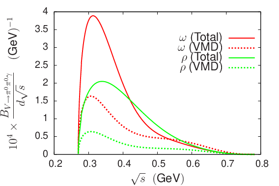
From this, and using the fitted parameters from the last line of table 1, we deduce the following results for the branching fractions
| (96) |
The result for the differs somewhat from that derived by the experimental groups [4, 5] (from the same data), being smaller by nearly one sigma. This illustrates that these branching fractions are not directly measurable quantities, unlike the cross-sections.
The shapes of the differential decay widths of the and the mesons, as a function of the energy, is illustrated on fig. 11. The two shapes are rather different. This can be easily understood from the general structure of the dispersive amplitudes (76). In the decay amplitude, a large rescattering contribution is induced from the Born terms integrals , which is absent in the isospin limit for the decay amplitude. Our result for is in better agreement with the one obtained using a unitarized ChPT approach [46] than those obtained using resonance models with a Breit-Wigner -meson (see fig. 11).
Finally, let us quote our results for the decays into . In this case, the Born amplitude contributes and one must take the infrared divergence into account. We follow ref. [67] and consider the radiative width defined with a cutoff on the photon energy MeV. Integrating the differential decay width (95) up to we obtain
| (97) |
The Born amplitude dominates this mode in the case of the decay. In the case of decay, the Born amplitude is suppressed by isospin but its relative contribution is nevertheless sizable. The experimental values for these branching fractions are [29]
| (98) |

6.2 Generalized polarizabilities
In the case where , it is fruitful to introduce the notion of generalized polarizabilities. This was originally proposed in the case of the nucleon in ref. [68] and extended to the case of the pion and further discussed in refs. [22, 23]. As explained in ref. [23], the generalized polarizabilities characterize the spatial distribution in the hadron of the polarizability induced by an external static electric or magnetic field. These observables can be related to the coefficient functions , , in the limit , after subtracting the Born term. We will be concerned here with the polarizability difference, which is given by [22]
| (99) |
( is denoted as in ref. [22]). Considering the expression for the helicity amplitude in terms of the coefficient functions (18) one sees that the polarizability difference can be related to the helicity amplitude taken in the limit ,
| (100) |
The results deriving from our dispersive amplitudes are shown in fig. 12 and compared to the chiral NLO results. Those have the simple expressions [22]
| (101) |
Keeping in mind that the values at in the dispersive amplitudes have been chosen to be slightly different from the chiral NLO values, fig. 12 shows that the variation as a function of of the generalized polarizabilities is described by the simple NLO expressions (101) to a rather good approximation.

6.3 Sigma meson electromagnetic form factor
The meson resonance is often used as a simplified description of the dynamics of re-scattering in the isoscalar -wave. From this point of view, electromagnetic properties of this resonance play a role in the hadronic contributions to the muon . For instance, in ref. [70] a contribution to the vacuum polarization was estimated assuming a vector dominance behaviour for the form factor. This form factor would also be involved if one considered the pole contribution in the light-by-light scattering amplitude. In the approach used here, the rescattering dynamics is expressed in terms of the partial-wave -matrix. The sigma meson can be identified as a pole of this function, in the complex energy plane, on the second Riemann sheet. It was shown in ref. [72] that a rather precise determination can be achieved, based on the Roy equations, despite the fact that this resonance has a rather large width. Further work on this topic was done in ref. [73].


The discontinuity/unitarity relation shows that the second sheet poles of the -matrix are also present in production amplitudes such as , . The determination of the dependent form factor from the latter amplitude can be performed in exactly the same way as that of the coupling constant from the former amplitude [24] using the residues of the second-sheet poles,
| (102) |
This definition would correspond to the following matrix element of the electromagnetic current in the zero width limit for the ,
| (103) |
Using eq. (102), together with the fact that corresponds to a zero of the -matrix on the first sheet, on obtains
| (104) |
with . We use here an -matrix constrained by the Roy equation up to the threshold discussed in [56], which gives (central values),
| (105) |
At , firstly, we obtain from the amplitude (76), (90) the to two photons coupling
| (106) |
in reasonable agreement with our previous result [56] ( MeV) based on a coupled channel Omnès representation and a more complete description of the left-hand cut. The variation as a function of is illustrated on fig. 13 which shows the ratio , separately for and . In a simple vector dominance picture, this ratio is expected to be proportional to for negative implying that should be real in this region. Fig. 13 shows that the actual results do not follow this simple VMD picture.
6.4 Contribution to the muon anomalous magnetic moment
Let us consider, finally, the contribution from the cross-section to the anomalous magnetic moment of the muon, . This contribution was discussed, in the case of charged pions, in refs. [69, 76] in the so called sQED approximation, which corresponds to retaining only the Born terms in the expression of amplitude. In the context of , the range of validity of our amplitude allows us to evaluate the corresponding contribution in the range GeV. Generically, these contributions to have the following form
| (107) |
where the kernel function is compactly expressed as [74]
| (108) |
(see e.g. [75] for the analytic expression and a detailed review).
In the case of charged pions, at first, one must take care of the infrared divergence. This may be done by separating the contribution from the Born amplitude squared
| (109) |
in the general expression for the cross-section (26) and correspondingly writing the cross-section as a sum of three terms
| (110) |
Only the first term in eq. (110) is affected by an infrared divergence. For definiteness, let us consider the inclusive definition, where is defined by combining it with the radiative correction to the vertex , and can then be written as follows
| (111) |
(see e.g. ref. [75] where the explicit expression for the function can be found). In accordance with the decomposition (110) of the cross-section we can write the contributions from to the muon anomalous magnetic moment as
| (112) |
and we find the following numerical results
| (113) |
showing the separate contributions from the three terms in eq. (110). Similarly, we can compute the contribution to the muon anomalous magnetic moment from the neutral channel , and we find
| (114) |
As was noted in the literature [69, 76, 77]) the contribution of the channel from the purely Born terms, is not negligible. It is of the same size as the present error in the Standard Model evaluation [78], . Comparatively, the other contributions from are rather small, even though they do include some enhancement from the strong rescattering in the isoscalar -wave. As an effect of rescattering, the contribution from the term linear in the Born amplitude (second term in eq. (110)) is found to be positive here, contrary to the result of [7]. Our evaluation of (113), (114) should be more precise than the estimates using -meson approximations [70, 71].
7 Conclusions
We have discussed the generalization of dispersive Omnès-type representations of amplitudes (as e.g. in refs. [17, 18]) to the case where one photon is virtual. These approaches involve a modelling of the left-hand cut, beyond the pion pole contribution, in terms of light resonance exchanges. We showed how this can be consistently defined as a generalized left-hand cut, with no intersection with the unitarity cut, through the use of a Källen-Lehmann representation for the resonance propagators and the limiting prescriptions for energy variables. Our main result is a representation of (or ) helicity amplitudes, eq. (76) which is based on twice-subtracted dispersion relations for the partial-waves. The representation satisfies the soft photon theorem and displays explicitly the dependence on the phase-shifts, on the pion electromagnetic form factor and on form factors. It also involves two functions of the virtuality . These functions are constrained by matching with ChPT, through the values at and their relation to the pion polarizabilites. We then showed that a simple two parameter representation is adequate for reproducing the experimental data on . Eq. (76) is valid in a range of virtualities and energies not exceeding 1 GeV, such that scattering is essentially elastic and the phase-shifts of partial-waves may be neglected. In principle, it is possible to extend this kind of representation to somewhat higher energies where inelasticity is dominated by the single channel, by constructing numerical solutions to the coupled Muskhelishvili-Omnès equations.
As a first application, the behaviour of the generalized polarizability difference , as a function of , was derived. This function is found not to deviate much from the prediction of ChPT at NLO at negative . As a second application, results were deduced for vector meson decay amplitudes as well as the electromagnetic form factor. This latter object can be defined from the second sheet pole definition of the resonance and generalizes the coupling introduced in ref. [24]. The amplitudes participate in the hadronic vacuum polarization contribution to the muon . We have evaluated the contributions beyond the point-like approximation, which is usually accounted for.
Acknowledgements
I would like to thank Diogo Boito for his participation in the first stages of this project. Work supported in part by the European Community-Research Infrastructure Integrating Activity ”Study of Strongly Integrating Matter” (acronym HadronPhysics3, Grant Agreement n. 283286) under the Seventh Framework Programme of EU.
Appendices

Appendix A Vector resonance propagator with good analyticity properties
We give here an explicit representation for the resonance propagator given from eqs. (50) and (51) (see also [32]). In order to evaluate the integral (50) in analytic form, one must first compute the three zeros , of the denominator of . Approximate values are,
| (115) |
with . More precise values must be determined numerically. The spectral integral can then be expressed in terms of the loop function (see (73)), as
| (116) |
where the coefficient functions , , are given by
| (117) |
and satisfy . The poles in these functions cancel in , but they are present on the second Riemann sheet, which is easily seen using the second sheet extension of ,
| (118) |
Fig. 14 compares the real parts of and .
Appendix B Probing the dispersive formulae with simple triangle diagrams
We consider here simple triangle diagrams (fig. 15) as a toy model of rescattering. This allows one to check the absence of anomalous thresholds in the dispersive representation and the correctness of the prescriptions for calculating the real and imaginary parts of the amplitude. All particles in the diagrams are spinless but we take kinematical conditions analogous to those relevant for our problem. We take the mass of the particle associated with the vertical line to be and the other two masses to be . The amplitude can be expressed as a one-dimensional parametric integral,
| (119) |
It is easily verified that the denominator produces no singularity, the only singularities are contained in the logarithms. The real and imaginary parts of the amplitude, in the representation (119) correspond to integrating over the real part and the imaginary part of the logarithm. In order to define the proper sign for the imaginary parts the energy variable is considered as the limit of and similarly for the energy variable .

Let us now consider two cases for the masses
a) :
In this situation, the parametric representation simplifies to
| (120) |
Let us examine the dispersive representation in the variable . The discontinuity is easily found to be
| (121) |
with . The discontinuity has a structure similar to the QED Born term (31) (in particular, it has a singularity at ). The dispersive representation of the amplitude requires no subtraction and has the form
| (122) |
One can verify that the representation (122) is correct (i.e. the absence of an anomalous threshold), as it can be derived from (120) by making a simple change of variable. Splitting the integration range into two parts: and , one sets in the first range and in the second, with
| (123) |
We can rewrite this representation in a form which exhibits the symmetry in and , in terms of a difference of two integrals
| (124) |
with
| (125) |
This form is a simplified analog of the Born term rescattering piece in eq. (59). The function can be expressed analytically
| (126) |
Let us finally remark that the imaginary part of the amplitude does not necessarily coincide with the -discontinuity, depending on the value of . Indeed,
| (127) |
b) :
Let us now consider the unequal mass case. Starting from the
parametric representation (119) one obtains
the expression for the -discontinuity as,
| (128) |
where the function is the same which appears in the vector-exchange amplitude (41). Thus, the dispersion relation representation of reads,
| (129) |
We have not been able to derive this expression by making a simple change of variables as in the equal mass case. As a check of its correctness, we show below that the imaginary parts of the dispersive and parametric representations coincide. For the real parts, we checked their equality only numerically.
When using eq. (129) one must be careful in the evaluation of the real and imaginary parts of the amplitude. Unlike the case when , no imaginary part is generated from the denominator (because ). The function , on the other hand, has an imaginary part if . With real and the limit of , the proper definition of is
| (130) |
The explicit expressions for were given in eq. (43). Inserting this in the dispersive representation of the triangle amplitude (129) we get, for the imaginary part
| (131) |
Let us verify that this result coincides with the one obtained from the parametric representation. We can write the logarithm in the integrand in eq. (119) as a difference: . The zeros of the polynomial are given by
| (132) |
and has an imaginary part when and . The zeros of the polynomial are given by
| (133) |
and has an imaginary part when and . Performing the integration over we find that eq. (119) gives
| (134) |
We can now compare eq. (134) with eq. (131): the two expressions are seen to be identical upon using the relations between the and the functions
| (135) |
The real part of the amplitude is more difficult to evaluate analytically, but one can verify numerically that the real parts of the dispersive and the parametric representations also coincide.
Appendix C Finiteness of at the threshold
We show here that no divergence affects the function (see (63)) at the threshold if one uses a two channel formalism. In connection with two-channel unitarity, one must use a Omnès matrix and the formula for becomes
| (136) |
which replaces eq. (63). The inverse of the Omnès matrix satisfies the following unitarity relation
| (137) |
where is the -matrix. By construction, multiplying the -matrix by the inverse of the Omnès function removes the right-hand cuts, so the matrix elements should not exhibit any cusp at the or the thresholds and therefore have continuous derivatives. The derivative of the remaining pieces involve
| (138) |
(with ) which give contributions which are finite and independent of .
Appendix D Electromagnetic form factors
D.1 Pion form factor
We need a description of the modulus and phase of the pion electromagnetic form factor . The form factor is defined from the matrix element in eq. (27). The modulus can be determined from experiment in the physical region () since it is related to the cross-section by the formula
| (139) |
at leading order in . Many such measurements have been performed recently, see e.g [79] and references therein. Accurate representations at medium energy can be obtained from a simple superposition of Breit-Wigner-type functions [80]. We use here the fit performed by the CMD-2 collaboration [81], based on the following representation,
| (140) |
In eq. (140), is the Gounaris-Sakurai function [30], which can be expressed as follows
| (141) |
with
| (142) |
and the loop function is given in eq. (73). For the meson, a simple Breit-Wigner function is used in eq. (140)
| (143) |
D.2 form factor
Naively, we expect that the form factor should be somewhat similar to the pion form factor, i.e. that it should be approximated reasonably well by a superposition of and resonances with a small isospin violating contribution from the . However, there could be some differences for two reasons: 1) the phase of is not related to the scattering phase , unlike the phase of of and 2) instability of the omega meson permits triangle diagram contributions to the form factor which violate real analyticity. In other terms, the discontinuity of the form factor along the elastic cut is complex. A dispersion relation analysis of which takes such effects into account was performed some time ago [82]. This was reconsidered more recently in ref. [83] whose dispersive analysis is based on self-consistent solutions of Khuri-Treiman type equations for the scattering amplitude [84]. As compared to these results, the Breit-Wigner type approach appears to be, at least qualitatively, acceptable and we will use it here because of its simplicity.
From an experimental point of view the form factor has been probed in the region GeV from [85, 86, 87, 88, 89] and from the decays by the CLEO collaboration [90]. It has also been measured in the energy region GeV from decays [91, 92, 93, 94, 95]. Let us first consider the and decay measurements. Experimental observables are related to the form factor by the following expressions
| (144) | |||
with . A dimensionless quantity also shown in ref. [90] is the spectral function which is given by
| (145) |
These experiments probe the “tail” of the resonance and can be reproduced in the region with a resonance superposition model very similar to that of
| (146) |
The parameter which describes mixing is taken to be the same as in . The parameter is not related to the corresponding one in because the phases of the form factors and should be allowed to be different. We perform a fit of the data varying the two parameters and the width of the resonance (fixing its mass to GeV [90]). We included 60 data points taken from refs. [87, 88, 89] in the fit and obtain the following values for the parameters
| (147) |
giving a . These results allow one to extract the value of the coupling constant (which will be useful below) from its relation with the coefficient of the Breit-Wigner function,
| (148) |
which gives (using MeV)
| (149) |
This value is somewhat smaller than the one obtained in the fits of ref. [88] (e.g. in fit I). This is because a) our fit is constrained to reproduce the PDG value of when (see eq. (38)) and b) our use of Gounaris-Sakurai functions for the , mesons. This indicates that there is a significant model dependent uncertainty in the determination of from . We account for this by multiplying the error in eq. (149) par a factor 10.

The result of this fit is illustrated on fig. 16 and on fig. 17 which also shows the energy region below the peak. One observes a reasonable agreement between our determined form factor and the data at low energies GeV but not with the few data points lying in the range GeV. The pole-like behaviour in this small region is a puzzle which cannot be explained by theoretical models [82, 83, 96]. A new decay experiment is being performed by the WASA at COSY collaboration [97] which will hopefully clarify the situation.

D.3 form factor
In principle, one could determine the form factor similarly to , using experimental inputs from scattering and decay. Unfortunately, the width of the resonance is much larger than that of the and this makes it much more difficult to extract unambiguously the cross section than it was for . There is also only an upper bound available for the decay amplitude . We will therefore try to estimate the form factor from (hopefully) plausible phenomenological considerations rather than from actual data. Let us start by writing, as before, a representation in terms of three Breit-Wigner functions (we ignore mixing here),
| (150) |
with and try to determine the parameters. The first one, , can be related to the coupling constant
| (151) |
and we can use its value determined above (149) (with a rescaled error, accounting for the model dependence), together with MeV and from the second line in eq. (37), which gives
| (152) |
We can write for the second parameter, , a relation analogous to eq. (151) and determine the coupling from . However, only the branching fraction for is precisely known, so we must content with a guess: which gives
| (153) |
The choice of the minus sign can be justified by the consideration of the mixing angle . Indeed, one expects (in a simple minded quark model picture) the following relation to hold
| (154) |
which requires the left-hand side to be negative if . This seems indeed to be the case if one determines from the vector meson masses, e.g. the quadratic mass formula gives . Our determined values for the couplings , gives a reasonably similar value: . This then leads to the following estimate for the parameter ,
| (155) |
while the last parameter in the representation (150) for is determined from the normalization condition . Finally, the result for the form factor is illustrated on fig. 18.

References
- [1] K. T. Engel, H. H. Patel and M. J. Ramsey-Musolf, Phys. Rev. D 86 (2012) 037502 [arXiv:1201.0809]
- [2] M. Hoferichter, private communication.
- [3] C. Carimalo, P. Kessler and J. Parisi, Phys. Rev. D 21 (1980) 669.
- [4] M. N. Achasov, K. I. Beloborodov, A. V. Berdyugin, A. G. Bogdanchikov, A. V. Bozhenok, D. A. Bukin, S. V. Burdin and A. V. Vasiljev et al., Phys. Lett. B 537 (2002) 201 [arXiv:hep-ex/0205068].
- [5] R. R. Akhmetshin et al. [CMD2 Collaboration], Phys. Lett. B 580 (2004) 119 [arXiv:hep-ex/0310012].
- [6] F. Ambrosino et al. [KLOE Collaboration], Eur. Phys. J. C 49 (2007) 473 [hep-ex/0609009].
- [7] S. Dubinsky, A. Korchin, N. Merenkov, G. Pancheri and O. Shekhovtsova, Eur. Phys. J. C 40 (2005) 41 [arXiv:hep-ph/0411113].
- [8] G. Pancheri, O. Shekhovtsova and G. Venanzoni, Phys. Lett. B 642 (2006) 342 [hep-ph/0605244].
- [9] S. Weinberg,“The Quantum Theory of Fields” vol. I, Cambridge University Press, p.130.
- [10] M. J. Creutz and M. B. Einhorn, Phys. Rev. D 1 (1970) 2537.
- [11] R. Omnès, Nuovo Cim. 8 (1958) 316.
- [12] N. I. Muskhelishvili,“Singular Integral Equations”, P. Noordhof, Groningen (1953).
- [13] M. Gourdin and A. Martin, Nuov. Cim. 17 (1960) 224.
- [14] C. E. Carlson and W. -K. Tung, Phys. Rev. D 4 (1971) 2873 [Erratum-ibid. D 6 (1972) 402].
- [15] O. Babelon, J. L. Basdevant, D. Caillerie, M. Gourdin and G. Mennessier, Nucl. Phys. B 114 (1976) 252.
- [16] D. Morgan and M. R. Pennington, Phys. Lett. B 192 (1987) 207.
- [17] D. Morgan and M. R. Pennington, Phys. Lett. B 272 (1991) 134.
- [18] J. F. Donoghue and B. R. Holstein, Phys. Rev. D 48 (1993) 137 [arXiv:hep-ph/9302203].
- [19] J. Bijnens and F. Cornet, Nucl. Phys. B 296 (1988) 557.
- [20] J. F. Donoghue, B. R. Holstein and Y. C. Lin Phys. Rev. D 37 (1988) 2423.
- [21] M. Hoferichter, D. R. Phillips and C. Schat, Eur. Phys. J. C 71 (2011) 1743 [arXiv:1106.4147].
- [22] C. Unkmeir, S. Scherer, A. I. L’vov and D. Drechsel, Phys. Rev. D 61 (2000) 034002 [arXiv:hep-ph/9904442].
- [23] A. I. L’vov, S. Scherer, B. Pasquini, C. Unkmeir and D. Drechsel, Phys. Rev. C 64 (2001) 015203 [arXiv:hep-ph/0103172].
- [24] M. R. Pennington, Phys. Rev. Lett. 97 (2006) 011601.
- [25] W. A. Bardeen and W. K. Tung, Phys. Rev. 173 (1968) 1423 [Erratum-ibid. D 4 (1971) 3229].
- [26] S. Bellucci, J. Gasser and M. E. Sainio, Nucl. Phys. B 423 (1994) 80 [Erratum-ibid. B 431 (1994) 413] [arXiv:hep-ph/9401206].
- [27] U. Bürgi, Nucl. Phys. B 479 (1996) 392 [arXiv:hep-ph/9602429].
- [28] M. Jacob and G. C. Wick, Annals Phys. 7 (1959) 404 [Annals Phys. 281 (2000) 774].
- [29] J. Beringer et al. [Particle Data Group Collaboration], Phys. Rev. D 86 (2012) 010001.
- [30] G. J. Gounaris and J. J. Sakurai, Phys. Rev. Lett. 21 (1968) 244.
- [31] G. Källen, Helvetica Physica Acta 25 (1952) 417, H. Lehmann, Nuov. Cim. 11 (1954) 342.
- [32] E. L. Lomon and S. Pacetti, Phys. Rev. D 85 (2012) 113004 [Erratum-ibid. D 86 (2012) 039901] [arXiv:1201.6126].
- [33] J. Kennedy and T. D. Spearman, Phys. Rev. 126 (1962) 1596.
- [34] F. E. Low, Phys. Rev. 110 (1958) 974.
- [35] H. Terazawa, Phys. Rev. Lett. 26 (1971) 1207.
- [36] J. Gasser and H. Leutwyler, Annals Phys. 158 (1984) 142.
- [37] P. Singer, Phys. Rev. 128 (1962) 2789.
- [38] P. Singer, Phys. Rev. 130 (1963) 2441.
- [39] F. M. Renard, Nuovo Cim. A 62 (1969) 475.
- [40] S. Fajfer and R. J. Oakes, Phys. Rev. D 42 (1990) 2392.
- [41] A. Bramon, A. Grau and G. Pancheri, Phys. Lett. B 283 (1992) 416.
- [42] K. Huber and H. Neufeld, Phys. Lett. B 357 (1995) 221 [hep-ph/9506257].
- [43] E. Marco, S. Hirenzaki, E. Oset and H. Toki, Phys. Lett. B 470 (1999) 20 [arXiv:hep-ph/9903217].
- [44] D. Guetta and P. Singer, Phys. Rev. D 63 (2001) 017502 [arXiv:hep-ph/0005059].
- [45] A. Bramon, R. Escribano, J. L. Lucio Martinez and M. Napsuciale, Phys. Lett. B 517 (2001) 345 [arXiv:hep-ph/0105179].
- [46] J. E. Palomar, S. Hirenzaki and E. Oset, Nucl. Phys. A 707 (2002) 161 [arXiv:hep-ph/0111308].
- [47] A. Gokalp, S. Solmaz and O. Yilmaz, Phys. Rev. D 67 (2003) 073007 [arXiv:hep-ph/0302129],A. Gokalp, A. Kucukarslan and O. Yilmaz, Phys. Rev. D 67 (2003) 073008 [arXiv:hep-ph/0302240].
- [48] R. Escribano, Phys. Rev. D 74 (2006) 114020 [arXiv:hep-ph/0606314].
- [49] S. Eidelman, S. Ivashyn, A. Korchin, G. Pancheri and O. Shekhovtsova, Eur. Phys. J. C 69 (2010) 103 [arXiv:1003.2141].
- [50] N. N. Achasov and A. V. Kiselev, Phys. Rev. D 83 (2011) 054008 [arXiv:1011.4446 [hep-ph]].
- [51] J. A. Oller and L. Roca, Eur. Phys. J. A 37 (2008) 15 [arXiv:0804.0309].
- [52] T. Mori et al. [Belle Collaboration], J. Phys. Soc. Jap. 76 (2007) 074102 [arXiv:0704.3538].
- [53] S. Uehara et al. [Belle Collaboration], Phys. Rev. D 78 (2008) 052004 [arXiv:0805.3387].
- [54] B. Ananthanarayan, G. Colangelo, J. Gasser and H. Leutwyler, Phys. Rept. 353 (2001) 207 [arXiv:hep-ph/0005297].
- [55] J. R. Batley et al. [NA48-2 Collaboration], Eur. Phys. J. C 70 (2010) 635.
- [56] B. Moussallam, Eur. Phys. J. C 71 (2011) 1814 [arXiv:1110.6074].
- [57] D. Babusci, S. Bellucci, G. Giordano, G. Matone, A. M. Sandorfi and M. A. Moinester, Phys. Lett. B 277 (1992) 158.
- [58] G. Amelino-Camelia, F. Archilli, D. Babusci, D. Badoni, G. Bencivenni, J. Bernabeu, R. A. Bertlmann and D. R. Boito et al., Eur. Phys. J. C 68 (2010) 619 [arXiv:1003.3868].
- [59] A. V. Guskov, Phys. Part. Nucl. Lett. 7 (2010) 192.
- [60] L. V. Filkov, I. Guiasu and E. E. Radescu, Phys. Rev. D 26 (1982) 3146.
- [61] B. Pasquini, D. Drechsel and S. Scherer, Phys. Rev. C 77 (2008) 065211 [arXiv:0805.0213 [hep-ph]].
- [62] J. Gasser, M. A. Ivanov and M. E. Sainio, Nucl. Phys. B 728 (2005) 31 [arXiv:hep-ph/0506265].
- [63] J. Gasser, M. A. Ivanov and M. E. Sainio, Nucl. Phys. B 745 (2006) 84 [arXiv:hep-ph/0602234].
- [64] R. Garcia-Martin and B. Moussallam, Eur. Phys. J. C 70 (2010) 155 [arXiv:1006.5373].
- [65] H. Marsiske et al. [Crystal Ball Collaboration], Phys. Rev. D 41 (1990) 3324.
- [66] N. Kaiser, Eur. Phys. J. A 47 (2011) 15.
- [67] S. I. Dolinsky, V. P. Druzhinin, M. S. Dubrovin, V. B. Golubev, V. N. Ivanchenko, E. V. Pakhtusova, A. N. Peryshkin and S. I. Serednyakov et al., Phys. Rept. 202 (1991) 99.
- [68] P. A. M. Guichon, G. Q. Liu and A. W. Thomas, Nucl. Phys. A 591 (1995) 606 [arXiv:nucl-th/9605031].
- [69] J. F. De Troconiz and F. J. Yndurain, Phys. Rev. D 65 (2002) 093001 [hep-ph/0106025].
- [70] S. Narison, Phys. Lett. B 568 (2003) 231 [arXiv:hep-ph/0303004].
- [71] A. I. Ahmadov, E. A. Kuraev and M. K. Volkov, Phys. Part. Nucl. Lett. 7 (2010) 334 [arXiv:1002.1797 [hep-ph]].
- [72] I. Caprini, G. Colangelo and H. Leutwyler, Phys. Rev. Lett. 96 (2006) 132001 [arXiv:hep-ph/0512364].
- [73] R. Garcia-Martin, R. Kaminski, J. R. Pelaez, J. Ruiz de Elvira and , Phys. Rev. Lett. 107 (2011) 072001 [arXiv:1107.1635].
- [74] B. E. Lautrup and E. De Rafael, Nucl. Phys. B 70 (1974) 317 [Erratum-ibid. B 78 (1974) 576].
- [75] F. Jegerlehner and A. Nyffeler, Phys. Rept. 477 (2009) 1 [arXiv:0902.3360 [hep-ph]].
- [76] K. Melnikov, Int. J. Mod. Phys. A 16 (2001) 4591 [hep-ph/0105267].
- [77] H. Czyz, A. Grzelinska, J. H. Kuhn and G. Rodrigo, Eur. Phys. J. C 33 (2004) 333 [hep-ph/0308312].
- [78] M. Davier, A. Hoecker, B. Malaescu and Z. Zhang, Eur. Phys. J. C 71 (2011) 1515 [Erratum-ibid. C 72 (2012) 1874] [arXiv:1010.4180 [hep-ph]].
- [79] J. P. Lees et al. [BaBar Collaboration], Phys. Rev. D 86 (2012) 032013 [arXiv:1205.2228 [hep-ex]].
- [80] J. H. Kühn and A. Santamaria, Z. Phys. C 48 (1990) 445.
- [81] R. R. Akhmetshin et al. [CMD-2 Collaboration], Phys. Lett. B 648 (2007) 28 [arXiv:hep-ex/0610021].
- [82] G. Koepp, Phys. Rev. D 10 (1974) 932.
- [83] S. P. Schneider, B. Kubis and F. Niecknig, Phys. Rev. D 86 (2012) 054013 [arXiv:1206.3098].
- [84] F. Niecknig, B. Kubis and S. P. Schneider, Eur. Phys. J. C 72 (2012) 2014 [arXiv:1203.2501].
- [85] S. I. Dolinsky et al., Phys. Lett. B 174 (1986) 453.
- [86] D. Bisello et al. [DM2 Collaboration], Nucl. Phys. Proc. Suppl. 21 (1991) 111.
- [87] M. N. Achasov, K. I. Beloborodov, A. V. Berdyugin, A. G. Bogdanchikov, A. V. Bozhenok, D. A. Bukin, S. V. Burdin and V. B. Golubev et al., Phys. Lett. B 486 (2000) 29 [arXiv:hep-ex/0005032].
- [88] R. R. Akhmetshin et al. [CMD-2 Collaboration], Phys. Lett. B 562 (2003) 173 [arXiv:hep-ex/0304009].
- [89] M. N. Achasov et al., JETP Lett. 94 (2012) 2.
- [90] K. W. Edwards et al. [CLEO Collaboration], Phys. Rev. D 61 (2000) 072003 [arXiv:hep-ex/9908024].
- [91] R. I. Dzhelyadin, S. V. Golovkin, A. S. Konstantinov, V. F. Konstantinov, V. P. Kubarovsky, L. G. Landsberg, V. A. Mukhin and V. F. Obraztsov et al., Phys. Lett. B 102 (1981) 296 [JETP Lett. 33 (1981) 228].
- [92] L. G. Landsberg, Phys. Rept. 128 (1985) 301.
- [93] R. R. Akhmetshin et al. [CMD-2 Collaboration], Phys. Lett. B 613 (2005) 29 [arXiv:hep-ex/0502024].
- [94] M. N. Achasov, K. I. Beloborodov, A. V. Berdyugin, A. G. Bogdanchikov, A. D. Bukin, D. A. Bukin, A. V. Vasilev and V. B. Golubev et al., J. Exp. Theor. Phys. 107 (2008) 61.
- [95] R. Arnaldi et al. [NA60 Collaboration], Phys. Lett. B 677 (2009) 260
- [96] C. Terschlüsen, S. Leupold and M. F. M. Lutz, [arXiv:1204.4125].
- [97] S. Schadmand [WASA-at-COSY Collaboration], PoS QNP 2012 (2012) 128.