跳到论文正文
W Papers独立论文阅读器 arXiv:1305.3030 论文正文 计算阅读时间 · 0%
引用这篇论文根据当前论文元数据生成,正式投稿前建议核对。


License: arXiv.org perpetual non-exclusive license
arXiv:1305.3030v3 [math-ph] 19 Jun 2013

Vertex models, TASEP and Grothendieck Polynomials

Kohei Motegi ††thanks: E-mail: motegi@gokutan.c.u-tokyo.ac.jp Affiliation: Okayama Institute for Quantum Physics, Kyoyama 1-9-1, Okayama 700-0015, Japan    Kazumitsu Sakai ††thanks: E-mail: sakai@gokutan.c.u-tokyo.ac.jp Affiliation: Institute of physics, University of Tokyo,Komaba 3-8-1, Meguro-ku, Tokyo 153-8902, Japan
May 14, 2013
Abstract

We examine the wavefunctions and their scalar products of a one-parameter family of integrable five vertex models. At a special point of the parameter, the model investigated is related to an irreversible interacting stochastic particle system the so-called totally asymmetric simple exclusion process (TASEP). By combining the quantum inverse scattering method with a matrix product representation of the wavefunctions, the on/off-shell wavefunctions of the five vertex models are represented as a certain determinant form. Up to some normalization factors, we find the wavefunctions are given by Grothendieck polynomials, which are a one-parameter deformation of Schur polynomials. Introducing a dual version of the Grothendieck polynomials, and utilizing the determinant representation for the scalar products of the wavefunctions, we derive a generalized Cauchy identity satisfied by the Grothendieck polynomials and their duals. Several representation theoretical formulae for Grothendieck polynomials are also presented. As a byproduct, the relaxation dynamics such as Green functions for the periodic TASEP are found to be described in terms of Grothendieck polynomials.

PACS numbers: 02.30.Ik, 02.50.Ey, 03.65.Fd

1 Introduction

Symmetric polynomials [1] are ubiquitous objects in mathematics and mathematical physics. One of the most basic and important symmetric polynomials is the Schur polynomials

sλ​(𝒛)=detN​(zjλk+N−k)∏1≤j<k≤N(zj−zk),\displaystyle s_{\lambda}(\boldsymbol{z})=\frac{\mathrm{det}_{N}(z_{j}^{\lambda_{k}+N-k})}{\prod_{1\leq j<k\leq N}(z_{j}-z_{k})}, (1.1)

where 𝒛={z1,…,zN}\boldsymbol{z}=\{z_{1},\dots,z_{N}\} is a set of variables and λ=(λ1,λ2,…,λN)\lambda=(\lambda_{1},\lambda_{2},\dots,\lambda_{N}) is a sequence of weakly decreasing nonnegative integers λ1≥λ2≥⋯≥λN≥0\lambda_{1}\geq\lambda_{2}\geq\dots\geq\lambda_{N}\geq 0. A sequence λ\lambda can be represented as a Young diagram whose kkth row has λk\lambda_{k} boxes.

Schur polynomials appear not only in representation theory but also in many contexts in mathematical physics, especially in integrable systems. For example, the tau functions of the KP hierarchy have Schur polynomial expansions [2]. Schur polynomials also appear as the singular vectors in conformal field theory [3, 4], the Green function of the vicious walkers [5, 6], the domain wall boundary partition function of the six vertex model [7, 8], the Schur processes as one of the most fundamental examples of determinantal processes [9], to list a few. The relation between integrable models and symmetric polynomials can be extended from Schur polynomials to Jack, Hall-Littlewood, Macdonald polynomials and so on.

In this paper, we develop a novel relation between integrable models and symmetric polynomials. We consider a family of integrable five vertex models. At a special point of the parameter, the model we investigate is related to an irreversible interacting stochastic particle system called the totally asymmetric simple exclusion process (TASEP) [10, 11, 12, 13, 14, 15]. At another point, the vertex models reduce to the four vertex model describing the one-dimensional quantum Ising model [16].

We show that up to normalization factors, the wavefunctions of the five vertex model are given by the Grothendieck polynomials [17, 18, 19]

Gλ​(𝒛,β)=detN​(zjλk+N−k​(1+β​zj)k−1)∏1≤j<k≤N(zj−zk),\displaystyle G_{\lambda}(\boldsymbol{z};\beta)=\frac{\mathrm{det}_{N}(z_{j}^{\lambda_{k}+N-k}(1+\beta z_{j})^{k-1})}{\prod_{1\leq j<k\leq N}(z_{j}-z_{k})}, (1.2)

which is a one-parameter extension of the Schur polynomials. The Grothendieck polynomial was originally introduced [17] in the context of the intersection between geometry and representation theory as a KK-theoretical extension of the Schubert polynomials, i.e. as polynomial representatives of Schubert classes in the Grothendieck ring of the flag manifold. The formal parameter β\beta corresponds to the KK-theoretical extension. For flag varieties of type AA, Schubert polynomials is the Schur polynomials itself, and it was shown recently [18, 19] that Grothendieck polynomials for flag varieties of type AA is expressed in the determinant form (1.2). We show the equivalence between the wavefunctions and Grothendieck polynomials by combining the quantum inverse scattering method with a matrix product representation of the wavefunctions. We find the wavefunctions correspond to the Grothendieck polynomials (1.2), and the dual wavefunctions to the following “dual” Grothendieck polynomials

G¯λ​(𝒛,β)=detN​(zjλk+N−k​(1+β​zj−1)1−k)∏1≤j<k≤N(zj−zk).\displaystyle\overline{G}_{\lambda}(\boldsymbol{z};\beta)=\frac{\mathrm{det}_{N}(z_{j}^{\lambda_{k}+N-k}(1+\beta z_{j}^{-1})^{1-k})}{\prod_{1\leq j<k\leq N}(z_{j}-z_{k})}. (1.3)

From this relation between integrable models and symmetric polynomials, we note that studying integrable five vertex models lead us to representation theoretical results of the Grothendieck polynomials. We present several results for the Grothendieck polynomials in this way, i.e. by studying the integrable five vertex models. We find the following Cauchy identity for the Grothendieck and dual Grothendieck polynomials

∑λ⊆(M−N)NGλ​(𝒛,β)​G¯λ​(𝒚,β)\displaystyle\sum_{\lambda\subseteq(M-N)^{N}}G_{\lambda}(\boldsymbol{z};\beta)\overline{G}_{\lambda}(\boldsymbol{y};\beta)
=∏1≤j<k≤N1(zj−zk)​(yj−yk)​detN​[(zj​yk)M−{(1+β​zj)/(1+β​yk−1)}N−1zj​yk−1],\displaystyle\qquad=\prod_{1\leq j<k\leq N}\frac{1}{(z_{j}-z_{k})(y_{j}-y_{k})}\mathrm{det}_{N}\left[\frac{(z_{j}y_{k})^{M}-\left\{(1+\beta z_{j})/(1+\beta y_{k}^{-1})\right\}^{N-1}}{z_{j}y_{k}-1}\right], (1.4)

which generalizes the one for Schur polynomials. We show this identity by evaluating the scalar products of the wavefunctions in two ways. We can evaluate the determinant representation of the scalar products directly in a way by use of the recursive relations called the Izergin-Korepin approach. The scalar products can also be evaluated by inserting the completeness relation and the determinant forms of the wavefunctions and dual wavefunctions. The two ways of the evaluation of the scalar products turns out to yield the Cauchy identity for Grothendieck polynomials (1.4). In short, we find a generalization of the celebrated Cauchy identity by analyzing a family of integrable five vertex models with the recently developed techniques to analyze integrable models (see [20, 21] for the six vertex model, [22, 23, 24, 25, 28] for the XXZ chain, and [27] for the totally asymmetric simple exclusion process). As a special case of the Cauchy identity, we also obtain the summation formula for the Grothendieck polynomials. There are several results on the generalizations of the Cauchy identity for symmetric polynomials related to geometry in the past (see [28, 29] for example). The one for the Grothendieck polynomials presented in this paper has advantages in that the connection with the Schur polynomials is explicit and easily understandable, which seems not to be known before.

As a byproduct of the determinant forms of the wavefunctions, we formulate the exact relaxation dynamics of the periodic TASEP for arbitrary initial condition, generalizing the case for the step and alternating initial conditions [30, 31].

This paper is organized as follows. In the next section, we introduce a one-parameter family of integrable five vertex models by solving the R​L​LRLL-relation, a version of the Yang-Baxter relation which guarantees the integrability of the model. In section 3, we evaluate the scalar products by the Izergin-Korepin approach to find its determinant form. In section 4, by combining the quantum inverse scattering method with a matrix product representation of the wavefunctions, the determinant representation of the wavefunctions is obtained. In section 5, we establish the relation between the wavefunctions and the Grothendieck polynomials. Combining the results in section 3 and 4, we derive the Cauchy identity and the summation formula for Grothendieck polynomials. We give a formulation of the exact relaxation dynamics of the periodic TASEP for arbitrary initial condition in section 6. Section 7 is devoted to the conclusion of this paper.

2 One-parameter family of five vertex models

A key ingredient in constructing quantum integrable models is to find a solution of the relation (R​L​LRLL-relation)

Rμ​ν​(u,v)​Lμ​j​(u)​Lν​j​(v)=Lν​j​(v)​Lμ​j​(u)​Rμ​ν​(u,v)\displaystyle R_{\mu\nu}(u,v)L_{\mu j}(u)L_{\nu j}(v)=L_{\nu j}(v)L_{\mu j}(u)R_{\mu\nu}(u,v) (2.1)

holding in End⁡(Wμ⊗Wν⊗Vj)\End(W_{\mu}\otimes W_{\nu}\otimes V_{j}) for arbitrary u,v∈ℂu,v\in\mathbb{C}. Here the matrix Rμ​ν​(u,v)∈End⁡(Wμ⊗Wν)R_{\mu\nu}(u,v)\in\End(W_{\mu}\otimes W_{\nu}) satisfies the Yang-Baxter equation

Rμ​ν​(u,v)​Rμ​γ​(u,w)​Rν​γ​(v,w)=Rν​γ​(v,w)​Rμ​γ​(u,w)​Rμ​ν​(u,v)\displaystyle R_{\mu\nu}(u,v)R_{\mu\gamma}(u,w)R_{\nu\gamma}(v,w)=R_{\nu\gamma}(v,w)R_{\mu\gamma}(u,w)R_{\mu\nu}(u,v) (2.2)

and Lμ​j​(u)L_{\mu j}(u) is an operator acting on the space Wμ⊗VjW_{\mu}\otimes V_{j}. By convention we call WW and VV the auxiliary space and the quantum space, respectively.

In the following, we shall take both of the spaces WW and VV to be the two-dimensional vector spaces W=V=ℂ2W=V=\mathbb{C}^{2} spanned by the “empty state” |0⟩=(10)|0\rangle=\binom{1}{0} and the “particle occupied state” |1⟩=(01)|1\rangle=\binom{0}{1}. (Note that WμW_{\mu} (resp. VjV_{j}) denotes a copy of ℂ2\mathbb{C}^{2} spanned by the μ\muth (resp. jjth) states |0⟩μ|0\rangle_{\mu} and |1⟩μ|1\rangle_{\mu} (resp. |0⟩j|0\rangle_{j} and |1⟩j|1\rangle_{j})). One solution to the Yang-Baxter equation (2.2) is the following RR-matrix whose elements are the Boltzmann weights associated with a five vertex model:

R⁡(u,v)=(f⁡(v,u)00000g⁡(v,u)00g⁡(v,u)10000f⁡(v,u))\displaystyle R(u,v)=\begin{pmatrix}f(v,u)&0&0&0\\ 0&0&g(v,u)&0\\ 0&g(v,u)&1&0\\ 0&0&0&f(v,u)\end{pmatrix} (2.3)

with

f⁡(v,u)=u2u2−v2,g⁡(v,u)=u​vu2−v2.\displaystyle f(v,u)=\frac{u^{2}}{u^{2}-v^{2}},\quad g(v,u)=\frac{uv}{u^{2}-v^{2}}. (2.4)

As a solution of the R​L​LRLL-relation (2.1) with the RR-matrix (2.3), we find the following LL-operator L⁡(u)∈End⁡(ℂ2⊗ℂ2)L(u)\in\End(\mathbb{C}^{2}\otimes\mathbb{C}^{2}) (see Appendix A for the detailed derivation):

Lμ​j​(u)=u​sμ​sj+σμ−​σj++σμ+​σj−+(α​u−u−1)​nμ​sj+α​u​nμ​nj,\displaystyle L_{\mu j}(u)=us_{\mu}s_{j}+\sigma_{\mu}^{-}\sigma_{j}^{+}+\sigma_{\mu}^{+}\sigma_{j}^{-}+(\alpha u-u^{-1})n_{\mu}s_{j}+\alpha un_{\mu}n_{j}, (2.5)

where σ±,σz\sigma^{\pm},\sigma^{z} are the spin-1/2 Pauli matrices; s=(1+σz)/2s=(1+\sigma^{z})/2 and n=(1−σz)/2n=(1-\sigma^{z})/2 are the projection operators onto the states |0⟩|0\rangle and |1⟩|1\rangle, respectively. Note that the operators with subscript μ\mu (resp. jj) act on the auxiliary (resp. quantum) space WμW_{\mu} (resp. VjV_{j}). See also Figure 1 for a pictorial description of the LL-operator (2.5), which allows for an intuitive understanding of the subsequent calculations.

The parameter α\alpha can be taken arbitrary11 1 Note that the parameter α\alpha is different from the parameter qq of a quantum group Uq​(s​l2)U_{q}(sl_{2}).. In fact, the models at special points of α\alpha are related to some physically interesting models. To see this, let us construct the monodromy matrix T⁡(u)T(u) by a product of LL-operators:

Tμ​(u)=∏i=1MLμ​j​(u)\displaystyle T_{\mu}(u)=\prod_{i=1}^{M}L_{\mu j}(u) (2.6)

which acts on Wμ⊗(V1⊗⋯⊗VM)W_{\mu}\otimes(V_{1}\otimes\dots\otimes V_{M}). Tracing out the auxiliary space, one defines the transfer matrix τ⁡(u)∈End⁡(V⊗M)\tau(u)\in\End(V^{\otimes M}):

τ⁡(u)=TrWμ⁡Tμ​(u).\displaystyle\tau(u)=\Tr_{W_{\mu}}T_{\mu}(u). (2.7)

Thanks to the R​L​LRLL-relation, the transfer matrix τ⁡(u)\tau(u) mutually commutes, i.e.

[τ⁡(u),τ⁡(v)]=0.\displaystyle[\tau(u),\tau(v)]=0. (2.8)

After taking the logarithmic derivative of the transfer matrix with respect to the spectral parameter, one obtains the quantum Hamiltonian which is, in general, non-Hermitian

ℋ:=∑j=1M{α​σj+​σj+1−+14​(σjz​σj+1z−1)}=12​α​∂∂u​log⁡{(α​u)−M​τ​(u)}|u=1α.\displaystyle\mathcal{H}:=\sum_{j=1}^{M}\left\{\alpha\sigma_{j}^{+}\sigma_{j+1}^{-}+\frac{1}{4}(\sigma_{j}^{z}\sigma_{j+1}^{z}-1)\right\}=\left.\frac{1}{2\sqrt{\alpha}}\frac{{\partial}}{{\partial}u}\log\left\{\left(\sqrt{\alpha}u\right)^{-M}\tau(u)\right\}\right|_{u=\frac{1}{\sqrt{\alpha}}}. (2.9)

At α=1\alpha=1, the LL-operator is essentially the same with the RR-matrix (2.3). In this case, the quantum Hamiltonian ℋ\mathcal{H} (2.9) can be interpreted as a stochastic matrix describing an irreversible interacting stochastic particle system called the totally asymmetric simple exclusion process (TASEP) [15, 27] (see section 6, for details). On the other hand, in the limit α→∞\alpha\to\infty, this model is related to an irreversible noncollisional diffusion process (i.e. a vicious random walker model): (ℋ/α−1)⊗N|α→∞(\mathcal{H}/\alpha-1)^{\otimes N}|_{\alpha\to\infty} is nothing but a transition matrix describing the process of NN vicious random walkers. Finally, the LL-operator at α=0\alpha=0 reduces to the four vertex model [16], and through the relation (2.9) it is related to the well-known Ising model.

The quantum integrability of the model (2.9) is easily understood by the commutativity of the transfer matrix (2.8) and its Hamiltonian limit (2.9): the transfer matrix τ⁡(u)\tau(u) is just a generator of nontrivial conserved quantities.

In the next section, by means of the quantum inverse scattering method, we construct state vectors of the Hamiltonian (2.9) (or equivalently, of the transfer matrix (2.7)), and calculate their scalar products.

Refer to caption
Figure 1: The non-zero elements of the LL-operator of the one-parameter family of five vertex models (2.5). The LL-operator is pictorially represented as two crossing arrows. The left (resp. up) arrow represents an auxiliary space (resp. a quantum space). The indices 0 or 1 on the left (resp. right) of the vertices denote the input (resp. output) states in the auxiliary space, while those on the bottom (resp. top) denote the input (resp. output) states in the quantum space.

3 Scalar Products of state vectors

Here we construct a state vector of the integrable models defined in the preceding section by using the quantum inverse scattering method (i.e the algebraic Bethe ansatz). The resultant NN-particle state |ψ⁡({u}N)⟩|\psi(\{u\}_{N})\rangle is characterized by NN unknown numbers uj∈ℂu_{j}\in\mathbb{C} (1≤j≤N1\leq j\leq N), which becomes an eigenstate of (2.9) (or (2.7)) if we choose the parameters {u}N\{u\}_{N} as an arbitrary set of solutions of certain algebraic equation (i.e. the Bethe ansatz equation, see (3.7)). Hereafter we call the eigenstates the on-shell states, while we call the states with arbitrary complex values of {u}N\{u\}_{N} the off-shell states. In this section, we construct the arbitrary off-shell states and show that their scalar products can be expressed as a determinant form.

First let us consider the monodromy matrix:

Tμ​(u,{w})=∏j=1MLμ​j​(u/wj)\displaystyle T_{\mu}(u,\{w\})=\prod_{j=1}^{M}L_{\mu j}(u/w_{j}) =(A⁡(u,{w})B⁡(u,{w})C⁡(u,{w})D⁡(u,{w}))μ.\displaystyle=\begin{pmatrix}A(u,\{w\})&B(u,\{w\})\\ C(u,\{w\})&D(u,\{w\})\end{pmatrix}_{\mu}. (3.1)

Here, for later convenience, we introduced the inhomogeneous parameters w1,…,wM∈ℂw_{1},\dots,w_{M}\in\mathbb{C}. Taking the homogeneous limit wj→1w_{j}\to 1 (1≤j≤M1\leq j\leq M), (2.6) is recovered:

T⁡(u,{w})|w1=1,…,wM=1=T⁡(u).\displaystyle T(u,\{w\})|_{w_{1}=1,\dots,w_{M}=1}=T(u). (3.2)

As in the above equation, hereafter we will omit {w}\{w\} for the quantities in the homogeneous limit (e.g. A⁡(u):=A⁡(u,{w})|w1=1,…,wM=1A(u):=A(u,\{w\})|_{w_{1}=1,\dots,w_{M}=1}). The four elements of the monodromy matrix A⁡(u,{w})A(u,\{w\}), etc. are the operators acting on the quantum space V1⊗⋯⊗VMV_{1}\otimes\dots\otimes V_{M}. The diagrammatic representations of these four elements are given by Figure. 2.

Refer to caption
Figure 2: The diagrammatic representation of the elements of the monodromy matrix (3.1) with the inhomogeneous parameters w1,…,wMw_{1},\dots,w_{M}.

Applying the R​L​LRLL-relation (2.1) repeatedly, the following intertwining relation

Rμ​ν​(u,v)​Tμ​(u,{w})​Tν​(v,{w})=Tν​(v,{w})​Tμ​(u,{w})​Rμ​ν​(u,v)\displaystyle R_{\mu\nu}(u,v)T_{\mu}(u,\{w\})T_{\nu}(v,\{w\})=T_{\nu}(v,\{w\})T_{\mu}(u,\{w\})R_{\mu\nu}(u,v) (3.3)

follows. The relations listed below are obtained by the above equation, which play a key role in the following calculations:

C⁡(u,{w})​B​(v,{w})=g⁡(u,v)​[A⁡(u,{w})​D​(v,{w})−A⁡(v,{w})​D​(u,{w})],\displaystyle C(u,\{w\})B(v,\{w\})=g(u,v)\left[A(u,\{w\})D(v,\{w\})-A(v,\{w\})D(u,\{w\})\right],
A⁡(u,{w})​B​(v,{w})=f⁡(u,v)​B​(v,{w})​A​(u,{w})+g⁡(v,u)​B​(u,{w})​A​(v,{w}),\displaystyle A(u,\{w\})B(v,\{w\})=f(u,v)B(v,\{w\})A(u,\{w\})+g(v,u)B(u,\{w\})A(v,\{w\}),
D⁡(u,{w})​B​(v,{w})=f⁡(v,u)​B​(v,{w})​D​(u,{w})+g⁡(u,v)​B​(u,{w})​D​(v,{w}),\displaystyle D(u,\{w\})B(v,\{w\})=f(v,u)B(v,\{w\})D(u,\{w\})+g(u,v)B(u,\{w\})D(v,\{w\}),
[B⁡(u,{w}),B⁡(v,{w})]=[C⁡(u,{w}),C⁡(v,{w})]=0.\displaystyle\left[B(u,\{w\}),B(v,\{w\})\right]=\left[C(u,\{w\}),C(v,\{w\})\right]=0. (3.4)

The transfer matrix τ⁡(u,{w})\tau(u,\{w\}) is then expressed as elements of the monodromy matrix:

τ⁡(u,{w})=TrWμ⁡Tμ​(u,{w})=A⁡(u,{w})+D⁡(u,{w}).\displaystyle\tau(u,\{w\})=\Tr_{W_{\mu}}T_{\mu}(u,\{w\})=A(u,\{w\})+D(u,\{w\}). (3.5)

The arbitrary NN-particle state |ψ⁡({u}N,{w})⟩|\psi(\{u\}_{N},\{w\})\rangle (resp. its dual ⟨ψ⁡({u}N,{w})|\langle\psi(\{u\}_{N},\{w\})|) (not normalized) with NN spectral parameters {u}N={u1,u2,…,uN}\{u\}_{N}=\{u_{1},u_{2},\dots,u_{N}\} is constructed by a multiple action of BB (resp. CC) operator on the vacuum state |Ω⟩:=|0M⟩:=|0⟩1⊗⋯⊗|0⟩M|\Omega\rangle:=|0^{M}\rangle:=|0\rangle_{1}\ \otimes\dots\otimes|0\rangle_{M} (resp. ⟨Ω|:=⟨0M|:=⟨0|⊗⋯⊗⟨0|M1\langle\Omega|:=\langle 0^{M}|:={}_{1}\langle 0|\otimes\dots\otimes{}_{M}\langle 0|):

|ψ⁡({u}N,{w})⟩=∏j=1NB⁡(uj,{w})​|Ω⟩,⟨ψ⁡({u}N,{w})|=⟨Ω|​∏j=1NC⁡(uj,{w}).\displaystyle|\psi(\{u\}_{N},\{w\})\rangle=\prod_{j=1}^{N}B(u_{j},\{w\})|\Omega\rangle,\quad\langle\psi(\{u\}_{N},\{w\})|=\langle\Omega|\prod_{j=1}^{N}C(u_{j},\{w\}). (3.6)

Due to the commutativity of the operators BB or CC (3.4), the states defined above (and also their scalar products) do not depend on the order of the product of BB or CC.

By the standard procedure of the algebraic Bethe ansatz, we have the followings.

Proposition 3.1.

The NN-particle state |ψ⁡({u}N,{w})⟩|\psi(\{u\}_{N},\{w\})\rangle and its dual ⟨ψ({u}N,{w})\langle\psi(\{u\}_{N},\{w\}) become an eigenstate (on-shell states) of the transfer matrix (3.5) when the set of parameters {u}N\{u\}_{N} satisfies the Bethe ansatz equation:

a⁡(uj,{w})d⁡(uj,{w})=−∏k=1Nf⁡(uk,uj)f⁡(uj,uk),\displaystyle\frac{a(u_{j},\{w\})}{d(u_{j},\{w\})}=-\prod_{k=1}^{N}\frac{f(u_{k},u_{j})}{f(u_{j},u_{k})}, (3.7)

where

a⁡(u,{w})=∏j=1Muwj,d⁡(u,{w})=∏j=1M(α​uwj−wju).\displaystyle a(u,\{w\})=\prod_{j=1}^{M}\frac{u}{w_{j}},\quad d(u,\{w\})=\prod_{j=1}^{M}\left(\frac{\alpha u}{w_{j}}-\frac{w_{j}}{u}\right). (3.8)

Then the eigenvalue of the transfer matrix is given by

τ⁡(u,{w})=a⁡(u,{w})​∏j=1Nf⁡(u,uj)+d⁡(u,{w})​∏j=1Nf⁡(uj,u).\displaystyle\tau(u,\{w\})=a(u,\{w\})\prod_{j=1}^{N}f(u,u_{j})+d(u,\{w\})\prod_{j=1}^{N}f(u_{j},u). (3.9)

The scalar product between the arbitrary off-shell state vectors, which is mainly considered in this section, is defined as

⟨ψ⁡({u}N,{w})|ψ⁡({v}N,{w})⟩=⟨Ω​|∏j=1NC⁡(uj,{w})​∏k=1NB⁡(vk,{w})|​Ω⟩\displaystyle\langle\psi(\{u\}_{N},\{w\})|\psi(\{v\}_{N},\{w\})\rangle=\langle\Omega|\prod_{j=1}^{N}C(u_{j},\{w\})\prod_{k=1}^{N}B(v_{k},\{w\})|\Omega\rangle (3.10)

with uj,vk∈ℂu_{j},v_{k}\in\mathbb{C}. In the homogeneous limit wj→1w_{j}\to 1 (1≤j≤N1\leq j\leq N), the following theorem is known [15, 22, 41].

Theorem 3.2.

The scalar product (3.10) in the homogeneous limit wj→1w_{j}\to 1 (1≤j≤N1\leq j\leq N) is given by a determinant form:

⟨ψ⁡({u}N)|ψ⁡({v}N)⟩=∏1≤j<k≤N1(uj2−uk2)​(vk2−vj2)​detN​Q​({u}N|{v}N),\displaystyle\langle\psi(\{u\}_{N})|\psi(\{v\}_{N})\rangle=\prod_{1\leq j<k\leq N}\frac{1}{(u_{j}^{2}-u_{k}^{2})(v_{k}^{2}-v_{j}^{2})}\mathrm{det}_{N}Q(\{u\}_{N}|\{v\}_{N}), (3.11)

where {u}N\{u\}_{N} and {v}N\{v\}_{N} are arbitrary sets of complex values (i.e. off-shell conditions), and QQ is an N×NN\times N matrix with matrix elements

Q​({u}N|{v}N)j​k=a⁡(uj)​d​(vk)​vk2​(N−1)−a⁡(vk)​d​(uj)​uj2​(N−1)vk/uj−uj/vk.\displaystyle Q(\{u\}_{N}|\{v\}_{N})_{jk}=\frac{a(u_{j})d(v_{k})v_{k}^{2(N-1)}-a(v_{k})d(u_{j})u_{j}^{2(N-1)}}{v_{k}/u_{j}-u_{j}/v_{k}}. (3.12)

Here we will show the above determinant formula by utilizing a method recently developed by Wheeler in the calculation of the scalar product of the spin-1/2 XXZ chain [25]. This technique is based on the Izergin-Korepin procedure [20, 21], which is originally a method to calculate the domain wall boundary partition function of the six vertex model [20, 21]. In contrast to the spin-1/2 XXZ chain, in our case there is no need to impose the Bethe ansatz equation (i.e. on-shell condition) to show the determinant formula. In other words, the determinant formula (3.11) is valid for arbitrary off-shell states.

What plays a fundamental role in this method is the following intermediate scalar products (see also Figure 3 for a diagrammatic representation)

S⁡({u}n​|{v}N|​{w})=⟨0M−N+n​1N−n|∏j=1nC⁡(uj,{w})​∏k=1NB⁡(vk,{w})|Ω⟩.\displaystyle S(\{u\}_{n}|\{v\}_{N}|\{w\})=\langle 0^{M-N+n}1^{N-n}|\prod_{j=1}^{n}C(u_{j},\{w\})\prod_{k=1}^{N}B(v_{k},\{w\})|\Omega\rangle. (3.13)

The term “intermediate” stems from the fact that (3.13) interpolates the scalar product (n=Nn=N) and the domain wall boundary partition function (n=0n=0).

Refer to caption
Figure 3: The graphical representation of the intermediate scalar products (3.13) with inhomogeneous parameters {w}\{w\}. The case n=Nn=N corresponds to the usual scalar product (3.10), while the case n=0n=0 corresponds to the domain wall boundary partition function.

We have the following lemma regarding the properties of the intermediate scalar product.

Lemma 3.3.

The intermediate scalar product (3.13) S⁡({u}n​|{v}N|​{w})S(\{u\}_{n}|\{v\}_{N}|\{w\}) satisfies the following properties.

  1. 1.

    S⁡({u}n​|{v}N|​{w})S(\{u\}_{n}|\{v\}_{N}|\{w\}) is symmetric with respect to the variables {w1,…,wM−N+n}\{w_{1},\dots,w_{M-N+n}\}.

  2. 2.

    ∏j=1nujM+2​n−2​N−1​S​({u}n​|{v}N|​{w})\prod_{j=1}^{n}u_{j}^{M+2n-2N-1}S(\{u\}_{n}|\{v\}_{N}|\{w\}) is a polynomial of degree M−N+n−1M-N+n-1 in un2u_{n}^{2}.

  3. 3.

    The following recursive relations between the intermediate scalar products hold

    S({u}n|{v}N|{w})|un=±α−1/2wM−N+n\displaystyle S(\{u\}_{n}|\{v\}_{N}|\{w\})|_{u_{n}=\pm\alpha^{-1/2}w_{M-N+n}}
    =αN−n−(M−1)/2​(±1)M−1​wM+n−NM∏j=1Mwj​S​({u}n−1​|{v}N|​{w}).\displaystyle\qquad\qquad=\alpha^{N-n-(M-1)/2}(\pm 1)^{M-1}\frac{w_{M+n-N}^{M}}{\prod_{j=1}^{M}w_{j}}S(\{u\}_{n-1}|\{v\}_{N}|\{w\}). (3.14)
  4. 4.

    The case n=0n=0 of the intermediate scalar products has the following form:

    S⁡({u}0​|{v}N|​{w})=αN⁡(N−1)/2​∏j=1N∏k=1M−N(α​vjwk−wkvj)​∏j=1NvjN−1∏j=M−N+1MwjN−1.\displaystyle S(\{u\}_{0}|\{v\}_{N}|\{w\})=\alpha^{N(N-1)/2}\prod_{j=1}^{N}\prod_{k=1}^{M-N}\left(\frac{\alpha v_{j}}{w_{k}}-\frac{w_{k}}{v_{j}}\right)\frac{\prod_{j=1}^{N}v_{j}^{N-1}}{\prod_{j=M-N+1}^{M}w_{j}^{N-1}}. (3.15)
Proof.

Property 1 follows from the R​L​LRLL-relation

R~j​k​(wj/wk)​Lμ​k​(u/wk)​Lμ​j​(u/wj)=Lμ​j​(u/wj)​Lμ​k​(u/wk)​R~j​k​(wj/wk)\displaystyle\widetilde{R}_{jk}(w_{j}/w_{k})L_{\mu k}(u/w_{k})L_{\mu j}(u/w_{j})=L_{\mu j}(u/w_{j})L_{\mu k}(u/w_{k})\widetilde{R}_{jk}(w_{j}/w_{k}) (3.16)

holding in End⁡(Wμ⊗Vj⊗VkCLOSE\End(W_{\mu}\otimes V_{j}\otimes V_{k}). Here R~\widetilde{R} is given by

R~​(u)=(u000001001α⁡(u−u−1)0000u),\displaystyle\widetilde{R}(u)=\begin{pmatrix}u&0&0&0\\ 0&0&1&0\\ 0&1&\alpha(u-u^{-1})&0\\ 0&0&0&u\end{pmatrix}, (3.17)

which intertwines the LL-operators acting on a common auxiliary space (but acting on different quantum spaces). Note the usual R​L​LRLL-relation (3.16) intertwines the LL-operators acting on a same quantum space but acting on different auxiliary spaces. The above R​L​LRLL-relation (3.17) allows one to construct the monodromy matrix as a product of the LL-operators acting on the same quantum space (see also the next section), and rewriting the intermediate scalar products in terms of the resultant monodromy matrices makes one see Property 1 holds.

Property 2 can be shown by inserting the completeness relation into the intermediate scalar products (see Figure 4 for a graphical interpretation)

S⁡({u}n​|{v}N|​{w})\displaystyle S(\{u\}_{n}|\{v\}_{N}|\{w\}) =⟨0M−N+n​1N−n|∏j=1nC⁡(uj,{w})​∏k=1NB⁡(vk,{w})|Ω⟩\displaystyle=\langle 0^{M-N+n}1^{N-n}|\prod_{j=1}^{n}C(u_{j},\{w\})\prod_{k=1}^{N}B(v_{k},\{w\})|\Omega\rangle
=∑k=1M−N+n⟨0M−N+n​1N−n|C⁡(un,{w})|0k−1​10M−N+n−k​1N−n⟩\displaystyle=\sum_{k=1}^{M-N+n}\langle 0^{M-N+n}1^{N-n}|C(u_{n},\{w\})|0^{k-1}10^{M-N+n-k}1^{N-n}\rangle
×⟨0k−1​10M−N+n−k​1N−n|∏j=1n−1C⁡(uj,{w})​∏k=1NB⁡(vk,{w})|Ω⟩,\displaystyle\qquad\times\langle 0^{k-1}10^{M-N+n-k}1^{N-n}|\prod_{j=1}^{n-1}C(u_{j},\{w\})\prod_{k=1}^{N}B(v_{k},\{w\})|\Omega\rangle, (3.18)

and noting the factor containing unu_{n} is calculated as

⟨0M−N+n​1N−n|C⁡(un,{w})|0k−1​10M−N+n−k​1N−n⟩\displaystyle\langle 0^{M-N+n}1^{N-n}|C(u_{n},\{w\})|0^{k-1}10^{M-N+n-k}1^{N-n}\rangle
=αN−n​unN−n+k−1∏j=1k−1wj​∏j=M−N+n+1Mwj​∏j=k+1M−N+n(α​unwj−wjun).\displaystyle\qquad\qquad\qquad\qquad=\frac{\alpha^{N-n}u_{n}^{N-n+k-1}}{\prod_{j=1}^{k-1}w_{j}\prod_{j=M-N+n+1}^{M}w_{j}}\prod_{j=k+1}^{M-N+n}\left(\frac{\alpha u_{n}}{w_{j}}-\frac{w_{j}}{u_{n}}\right). (3.19)
Refer to caption
Figure 4: The intermediate scalar products where the completeness relation is inserted (3.18). Note the parameter unu_{n} comes only from the top row.

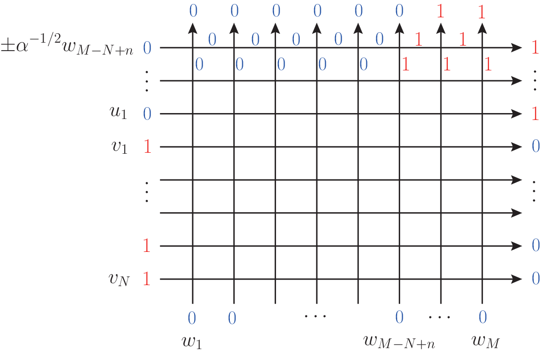
Property 3 can be obtained by setting un=±α−1/2wM−N+nu_{n}=\pm\alpha^{-1/2}w_{M-N+n} in (3.18), or can be directly observed by its graphical representation (Figure 5) that the top row is completely frozen.
Refer to caption
Figure 5: The graphical representation of the recursive relation (3.14). We can see that the top row is frozen by setting the spectral parameter unu_{n} to un=±α−1/2wM−N+nu_{n}=\pm\alpha^{-1/2}w_{M-N+n}.

Property 4 can be shown by noting that all the internal states are frozen (Figure 6), and reading out and multiplying all the weights of the LL-operators to find (3.15). ∎

Refer to caption
Figure 6: The intermediate scalar products (3.15) for n=0n=0, which corresponds to the domain wall boundary partition function. One sees all the internal states are frozen when the boundary states are fixed to the configuration in the figure.
Lemma 3.4.

The properties in Lemma 3.3 uniquely determine the intermediate scalar product (3.13).

Proof.

The proof is by induction on nn. For n=0n=0, by Property 4 the assertion is trivial. Assume by induction that the assertion holds for n−1n-1. Taking into account Property 1, one finds that Property 3 gives values of ∏j=1nujM+2​n−2​N−1​S​({u}n​|{v}N|​{w})\prod_{j=1}^{n}u_{j}^{M+2n-2N-1}S(\{u\}_{n}|\{v\}_{N}|\{w\}) at M−N+nM-N+n distinct points of un2u_{n}^{2}. By this together with Property 2, S⁡({u}n​|{v}N|​{w})S(\{u\}_{n}|\{v\}_{N}|\{w\}) is uniquely determined. Thus the assertion holds for nn. ∎

Due to Lemma 3.4, the following determinant representation for the intermediate scalar product is valid.

Theorem 3.5.

The intermediate scalar product S⁡({u}n​|{v}N|​{w})S(\{u\}_{n}|\{v\}_{N}|\{w\}) (3.13) has the following determinant form:

S⁡({u}n​|{v}N|​{w})=\displaystyle S(\{u\}_{n}|\{v\}_{N}|\{w\})= ∏M−N+n+1≤j<k≤M1wj2−wk2​∏1≤j<k≤n1uj2−uk2​∏1≤j<k≤N1vk2−vj2\displaystyle\prod_{M-N+n+1\leq j<k\leq M}\frac{1}{w_{j}^{2}-w_{k}^{2}}\prod_{1\leq j<k\leq n}\frac{1}{u_{j}^{2}-u_{k}^{2}}\prod_{1\leq j<k\leq N}\frac{1}{v_{k}^{2}-v_{j}^{2}}
×detN​Q​({u}n​|{v}N|​{w})\displaystyle\times\mathrm{det}_{N}Q(\{u\}_{n}|\{v\}_{N}|\{w\}) (3.20)

with an N×NN\times N matrix Q⁡({u}n​|{v}N|​{w})Q(\{u\}_{n}|\{v\}_{N}|\{w\}) whose matrix elements are given by

Q​({u}n​|{v}N|​{w})j​k\displaystyle Q(\{u\}_{n}|\{v\}_{N}|\{w\})_{jk}
={a⁡(uj,{w})​d​(vk,{w})​vk2​(N−1)−a⁡(vk,{w})​d​(uj,{w})​uj2​(N−1)(vk/uj−uj/vk)​∏l=M−N+n+1M(uj2−α−1​wl2), (1≤j≤n)vk2​(N−1)​∏l=1l≠M−N+jM(α​vkwl−wlvk), (n+1≤j≤N).\displaystyle\quad=\begin{cases}\frac{\displaystyle a(u_{j},\{w\})d(v_{k},\{w\})v_{k}^{2(N-1)}-a(v_{k},\{w\})d(u_{j},\{w\})u_{j}^{2(N-1)}}{\displaystyle(v_{k}/u_{j}-u_{j}/v_{k})\prod_{l=M-N+n+1}^{M}(u_{j}^{2}-\alpha^{-1}w_{l}^{2})},&\text{ ($1\leq j\leq n$)}\\ \displaystyle v_{k}^{2(N-1)}\prod_{\begin{subarray}{c}l=1\\ l\neq M-N+j\end{subarray}}^{M}\left(\frac{\alpha v_{k}}{w_{l}}-\frac{w_{l}}{v_{k}}\right),&\text{ ($n+1\leq j\leq N$)}\end{cases}. (3.21)
Proof.

We can directly see that the determinant formula (3.20) satisfies all the properties in Lemma 3.3. To show Property 2, we just use the fact that the singularities un2=uj2u_{n}^{2}=u_{j}^{2} (1≤j≤n−11\leq j\leq n-1) in the prefactor, and un2=α−1​wj2u_{n}^{2}=\alpha^{-1}w_{j}^{2} (M−N+n+1≤j≤MM-N+n+1\leq j\leq M) and un2=vj2u_{n}^{2}=v_{j}^{2} (1≤j≤n1\leq j\leq n) in elements of the determinant are removal. For Property 4, we utilize the Cauchy determinant formula to obtain

detN​{(α1/2​vkwM−N+j−wM−N+jα1/2​vk)−1}=∏M−N+1≤j<k≤M(wjwk−wkwj)​∏1≤j<k≤N(vkvj−vjvk)∏j=1N∏k=M−N+1M(α1/2​vjwk−wkα1/2​vj).\displaystyle\mathrm{det}_{N}\left\{\left(\frac{\alpha^{1/2}v_{k}}{w_{M-N+j}}-\frac{w_{M-N+j}}{\alpha^{1/2}v_{k}}\right)^{-1}\right\}=\frac{\displaystyle\prod_{M-N+1\leq j<k\leq M}\left(\frac{w_{j}}{w_{k}}-\frac{w_{k}}{w_{j}}\right)\prod_{1\leq j<k\leq N}\left(\frac{v_{k}}{v_{j}}-\frac{v_{j}}{v_{k}}\right)}{\displaystyle\prod_{j=1}^{N}\prod_{k=M-N+1}^{M}\left(\frac{\alpha^{1/2}v_{j}}{w_{k}}-\frac{w_{k}}{\alpha^{1/2}v_{j}}\right)}. (3.22)

Finally due to Lemma 3.4, the determinant formula (3.20) holds. ∎

Corollary 3.6.

Taking n=Nn=N in (3.20) yields the determinant representation of the scalar product for the five vertex model with inhomogeneous parameters (3.10):

⟨ψ⁡({u}N,{w})|ψ⁡({v}N,{w})⟩=\displaystyle\langle\psi(\{u\}_{N},\{w\})|\psi(\{v\}_{N},\{w\})\rangle= ∏1≤j<k≤n1(uj2−uk2)​(vk2−vj2)​detN​Q​({u}N​|{v}N|​{w})\displaystyle\prod_{1\leq j<k\leq n}\frac{1}{(u_{j}^{2}-u_{k}^{2})(v_{k}^{2}-v_{j}^{2})}\mathrm{det}_{N}Q(\{u\}_{N}|\{v\}_{N}|\{w\}) (3.23)

with

Q​({u}N​|{v}N|​{w})j​k=a⁡(uj,{w})​d​(vk,{w})​vk2​(N−1)−a⁡(vk,{w})​d​(uj,{w})​uj2​(N−1)vk/uj−uj/vk.\displaystyle Q(\{u\}_{N}|\{v\}_{N}|\{w\})_{jk}=\frac{a(u_{j},\{w\})d(v_{k},\{w\})v_{k}^{2(N-1)}-a(v_{k},\{w\})d(u_{j},\{w\})u_{j}^{2(N-1)}}{v_{k}/u_{j}-u_{j}/v_{k}}. (3.24)

Further taking the homogeneous limit wj→1w_{j}\to 1 (1≤j≤n1\leq j\leq n) yields (3.11) in Theorem 3.5.

The state vectors |ψ⁡({u}N)⟩|\psi(\{u\}_{N})\rangle and ⟨ψ⁡({u}N)|\langle\psi(\{u\}_{N})| become the energy eigenstates of (6.3), when an arbitrary set of solutions {u}N\{u\}_{N} to the Bethe ansatz equation (3.7) in the homogeneous limit wj→1w_{j}\to 1 (1≤j≤N1\leq j\leq N) is substituted into the state vectors. Then we have the following corollary regarding the norm of the eigenstates.

Corollary 3.7.

The norm of the eigenstates in the homogeneous limit wj→1w_{j}\to 1 (1≤j≤n1\leq j\leq n) is given by

⟨ψ⁡({u}N)|ψ⁡({u}N)⟩=∏j=1Nuj2​(M+N−1)​∏j,k=1j≠kN1uj2−uk2​detN​Q~​({u}N)\displaystyle\langle\psi(\{u\}_{N})|\psi(\{u\}_{N})\rangle=\prod_{j=1}^{N}u_{j}^{2(M+N-1)}\prod_{\begin{subarray}{c}j,k=1\atop j\neq k\end{subarray}}^{N}\ \frac{1}{u_{j}^{2}-u_{k}^{2}}\mathrm{det}_{N}\widetilde{Q}(\{u\}_{N}) (3.25)

with

Q~j​k​({u}N)=−1+α​N+(M−N)​uj−2α−uj−2​δj​k.\displaystyle\widetilde{Q}_{jk}(\{u\}_{N})=-1+\frac{\alpha N+(M-N)u_{j}^{-2}}{\alpha-u_{j}^{-2}}\delta_{jk}. (3.26)

By use of Sylvester’s determinant theorem, the determinant in the above further reduces to

detN​Q~=∏j=1Nα​N+(M−N)​uj−2α−uj−2​(1−∑j=1Nα−uj−2α​N+(M−N)​uj−2).\displaystyle\mathrm{det}_{N}\widetilde{Q}=\prod_{j=1}^{N}\frac{\alpha N+(M-N)u_{j}^{-2}}{\alpha-u_{j}^{-2}}\left(1-\sum_{j=1}^{N}\frac{\alpha-u_{j}^{-2}}{\alpha N+(M-N)u_{j}^{-2}}\right). (3.27)

4 Wavefunctions

In this section, we compute the overlap between an arbitrary off-shell NN-particle state |ψ⁡({u}N)⟩|\psi(\{u\}_{N})\rangle and the (normalized) state with an arbitrary particle configuration |x1⋯xN⟩|x_{1}\cdots x_{N}\rangle (x1<⋯<xNCLOSE(x_{1}<\dots<x_{N}), where xjx_{j} denotes the positions of the particles. Namely here we evaluate the wavefunction ⟨x1⋯xN|ψ({u}N)⟩\langle x_{1}\cdots x_{N}|\psi(\{u\}_{N})\rangle and its dual ⟨ψ⁡({u}N)|x1​…​xN⟩\langle\psi(\{u\}_{N})|x_{1}\dots x_{N}\rangle. One finds these quantities are crucial to describe physically interesting phenomena such as the relaxation dynamics as in Section 6, because the state |ψ​({u})N⟩|\psi(\{u\})_{N}\rangle becomes an eigenstate of the Hamiltonian (2.9) (correspondingly ⟨x1​…​xN|ψ⁡({u}N)⟩\langle x_{1}\dots x_{N}|\psi(\{u\}_{N})\rangle becomes an energy eigenfunction), if we choose {u}N\{u\}_{N} as an arbitrary set of solutions of the Bethe ansatz equation (see Proposition 3.1 and Section 6 for details). Here and in what follows, we consider the homogeneous case w1=1,…,wM=1w_{1}=1,\dots,w_{M}=1, and as noted in the previous section we omit {w}\{w\} as in (3.2).

The main results in this section are summarized in the following theorem.

Theorem 4.1.

The wavefunctions can be written as the following determinant formulae:

⟨x1⋯xN|ψ({v}N)⟩=∏j=1NvjM−1​(α​vj2−1)−1∏1≤j<k≤N(vk2−vj2)detN(vj2​k(α−vj−2)xk),\displaystyle\langle x_{1}\cdots x_{N}|\psi(\{v\}_{N})\rangle=\frac{\prod_{j=1}^{N}v_{j}^{M-1}(\alpha v_{j}^{2}-1)^{-1}}{\prod_{1\leq j<k\leq N}(v_{k}^{2}-v_{j}^{2})}\mathrm{det}_{N}(v_{j}^{2k}(\alpha-v_{j}^{-2})^{x_{k}}), (4.1)
⟨ψ({u}N)|x1⋯xN⟩=∏j=1N(α​uj−uj−1)M​uj2​N−1∏1≤j<k≤N(uj2−uk2)detN(uj−2​k(α−uj−2)−xk),\displaystyle\langle\psi(\{u\}_{N})|x_{1}\cdots x_{N}\rangle=\frac{\prod_{j=1}^{N}(\alpha u_{j}-u_{j}^{-1})^{M}u_{j}^{2N-1}}{\prod_{1\leq j<k\leq N}(u_{j}^{2}-u_{k}^{2})}\mathrm{det}_{N}(u_{j}^{-2k}(\alpha-u_{j}^{-2})^{-x_{k}}), (4.2)

where

⟨x1​…​xN|=⟨Ω|​∏j=1Nσxj+,|x1​…​xN⟩=∏j=1Nσxj−​|Ω⟩,\displaystyle\langle x_{1}\dots x_{N}|=\langle\Omega|\prod_{j=1}^{N}\sigma^{+}_{x_{j}},\qquad|x_{1}\dots x_{N}\rangle=\prod_{j=1}^{N}\sigma^{-}_{x_{j}}|\Omega\rangle, (4.3)

and {v}N\{v\}_{N} and {u}N\{u\}_{N} are sets of arbitrary complex parameters.

The strategy to show Theorem 4.1 is as follows. We first rewrite the wavefunctions into a matrix product form, following [27]. The matrix product form can be expressed as a determinant with some overall factor which remains to be calculated. The information of the particle configuration {x1,x2,…,xN}\{x_{1},x_{2},\dots,x_{N}\} is encoded in the determinant. On the other hand, the overall factor is independent of the particle positions, and therefore we can determine this factor by considering the specific configuration: we explicitly calculate it with the help of the result for the overlap of the consecutive configuration (i.e. xj=jx_{j}=j) obtained in [30, 31].

Let us begin to compute the wavefunctions. We consider (4.2) first. The proof of (4.1) can be done in a similar way. First we shall rewrite the wavefunction ⟨ψ({u}N|x1…xN⟩\langle\psi(\{u\}_{N}|x_{1}\dots x_{N}\rangle into the matrix product representation. With the help of graphical description, one finds that the wavefunction can be written as

⟨Ω|∏j=1NC(uj)|x1…xN⟩=TrW⊗N[⟨Ω|∏μ=1NTμ(uμ)|x1⋯xN⟩P],\displaystyle\langle\Omega|\prod_{j=1}^{N}C(u_{j})|x_{1}\dots x_{N}\rangle=\Tr_{W^{\otimes N}}\left[\langle\Omega|\prod_{\mu=1}^{N}T_{\mu}(u_{\mu})|x_{1}\cdots x_{N}\rangle P\right], (4.4)

where P=|0N⟩​⟨1N|P=|0^{N}\rangle\langle 1^{N}| is an operator acting on the tensor product of auxiliary spaces W1⊗⋯⊗WNW_{1}\otimes\dots\otimes W_{N}. The trace here is also over the auxiliary spaces. Due to the commutativity of the operators BB or CC (3.4), the wavefunctions do not depend on the order of the product of BB or CC. In other words, the wavefunctions are symmetric with respect to the parameters {u}N\{u\}_{N} or {v}N\{v\}_{N}. Changing the viewpoint of the products of the monodromy matrices, we have

∏μ=1NTμ​(uμ)=∏j=1M𝒯j​({u}N),\displaystyle\prod_{\mu=1}^{N}T_{\mu}(u_{\mu})=\prod_{j=1}^{M}\mathcal{T}_{j}(\{u\}_{N}), (4.5)

where 𝒯j​({u}N):=∏μ=1NLμ​j​(uμ)∈End⁡(W⊗N⊗Vj)\mathcal{T}_{j}(\{u\}_{N}):=\prod_{\mu=1}^{N}L_{\mu j}(u_{\mu})\in\End(W^{\otimes N}\otimes V_{j}) can be regarded as a monodromy matrix consisting of LL-operators acting on the same quantum space VjV_{j} (but acting on different auxiliary spaces). The monodromy matrix is decomposed as

𝒯j​({u}N)\displaystyle\mathcal{T}_{j}(\{u\}_{N}) :=(𝒜N​({u}N)ℬN​({u}N)𝒞N​({u}N)𝒟N​({u}N))j,\displaystyle:=\begin{pmatrix}\mathcal{A}_{N}(\{u\}_{N})&\mathcal{B}_{N}(\{u\}_{N})\\ \mathcal{C}_{N}(\{u\}_{N})&\mathcal{D}_{N}(\{u\}_{N})\end{pmatrix}_{j}, (4.6)

where the elements (𝒜N\mathcal{A}_{N}, etc.) act on W1⊗⋯⊗WNW_{1}\otimes\dots\otimes W_{N}. The wavefunction (4.4) can then be rewritten by 𝒯j​({u}N)\mathcal{T}_{j}(\{u\}_{N}) as

⟨ψ⁡({u}N)|x1​…​xN⟩\displaystyle\langle\psi(\{u\}_{N})|x_{1}\dots x_{N}\rangle =TrW⊗N[⟨Ω|∏j=1M𝒯j({u}N)|x1⋯xN⟩P]\displaystyle=\Tr_{W^{\otimes N}}\left[\langle\Omega|\prod_{j=1}^{M}\mathcal{T}_{j}(\{u\}_{N})|x_{1}\cdots x_{N}\rangle P\right]
=TrW⊗N⁡[𝒜NM−xN​ℬN​𝒜NxN−xN−1−1​…​ℬN​𝒜Nx2−x1−1​ℬN​𝒜Nx1−1​P].\displaystyle=\Tr_{W^{\otimes N}}\left[\mathcal{A}_{N}^{M-x_{N}}\mathcal{B}_{N}\mathcal{A}_{N}^{x_{N}-x_{N-1}-1}\dots\mathcal{B}_{N}\mathcal{A}_{N}^{x_{2}-x_{1}-1}\mathcal{B}_{N}\mathcal{A}_{N}^{x_{1}-1}P\right]. (4.7)

In Figure 7, we depict the elements 𝒜n​({u}n)\mathcal{A}_{n}(\{u\}_{n}) and ℬn​({u}n)\mathcal{B}_{n}(\{u\}_{n}) of the monodromy matrix 𝒯j​({u}n)\mathcal{T}_{j}(\{u\}_{n}), which explicitly appear in (4.7).

Refer to caption
Figure 7: The elements 𝒜⁡({u}n)\mathcal{A}(\{u\}_{n}) and ℬ⁡({u}n)\mathcal{B}(\{u\}_{n}) of the monodromy matrix 𝒯j​({u}n)\mathcal{T}_{j}(\{u\}_{n}) (4.6).

For these operators, one finds the following recursive relations:

𝒜n+1​({u}n+1)=𝒜n​({u}n)⊗(un+100α​un+1−un+1−1)+ℬn​({u}n)⊗(0100),\displaystyle\mathcal{A}_{n+1}(\{u\}_{n+1})=\mathcal{A}_{n}(\{u\}_{n})\otimes\begin{pmatrix}u_{n+1}&0\\ 0&\alpha u_{n+1}-u_{n+1}^{-1}\end{pmatrix}+\mathcal{B}_{n}(\{u\}_{n})\otimes\begin{pmatrix}0&1\\ 0&0\end{pmatrix}, (4.8)
ℬn+1​({u}n+1)=𝒜n​({u}n)⊗(0010)+ℬn​({u}n)⊗(000α​un+1)\displaystyle\mathcal{B}_{n+1}(\{u\}_{n+1})=\mathcal{A}_{n}(\{u\}_{n})\otimes\begin{pmatrix}0&0\\ 1&0\end{pmatrix}+\mathcal{B}_{n}(\{u\}_{n})\otimes\begin{pmatrix}0&0\\ 0&\alpha u_{n+1}\end{pmatrix} (4.9)

with the initial condition

𝒜1=(u100α​u1−u1−1),ℬ1=(0010).\displaystyle\mathcal{A}_{1}=\begin{pmatrix}u_{1}&0\\ 0&\alpha u_{1}-u_{1}^{-1}\end{pmatrix},\quad\mathcal{B}_{1}=\begin{pmatrix}0&0\\ 1&0\end{pmatrix}. (4.10)

See Figure 8 for a graphical description of the recursion relation for the operator 𝒜n​({u}n)\mathcal{A}_{n}(\{u\}_{n}).

Refer to caption
Figure 8: The graphical description of the recursive relation for the element 𝒜n​({u}n)\mathcal{A}_{n}(\{u\}_{n}) (see (4.8)).

By using the recursive relations (4.8) and (4.9), one sees that these operators satisfy the following simple algebra.

Lemma 4.2.

There exists a decomposition of ℬn\mathcal{B}_{n} : ℬn=∑j=1nℬn(j)\mathcal{B}_{n}=\sum_{j=1}^{n}\mathcal{B}_{n}^{(j)} such that the following algebraic relations hold for 𝒜n\mathcal{A}_{n} and ℬn(j)\mathcal{B}_{n}^{(j)}:

ℬn(j)​𝒜n=ujα​uj−uj−1​𝒜n​ℬn(j),\displaystyle\mathcal{B}_{n}^{(j)}\mathcal{A}_{n}=\frac{u_{j}}{\alpha u_{j}-u_{j}^{-1}}\mathcal{A}_{n}\mathcal{B}_{n}^{(j)}, (4.11)
(ℬn(j))2=0,\displaystyle(\mathcal{B}_{n}^{(j)})^{2}=0, (4.12)
(α​uj2−1)​ℬn(j)​ℬn(k)=−(α​uk2−1)​ℬn(k)​ℬn(j),(j≠k).\displaystyle(\alpha u_{j}^{2}-1)\mathcal{B}_{n}^{(j)}\mathcal{B}_{n}^{(k)}=-(\alpha u_{k}^{2}-1)\mathcal{B}_{n}^{(k)}\mathcal{B}_{n}^{(j)},\ \ \ (j\neq k). (4.13)
Proof.

This can be shown by induction on nn. For n=1n=1, from (4.10) 𝒜1\mathcal{A}_{1} is diagonal and one directly sees that the relations are valid. For nn, we assume that 𝒜n\mathcal{A}_{n} is diagonalizable and write the corresponding diagonal matrix as 𝒜n=Gn−1​𝒜n​Gn\mathscr{A}_{n}=G_{n}^{-1}\mathcal{A}_{n}G_{n}. Also writing ℬn=Gn−1​ℬn​Gn\mathscr{B}_{n}=G_{n}^{-1}\mathcal{B}_{n}G_{n} and ℬn=∑j=1nℬn(j)\mathscr{B}_{n}=\sum_{j=1}^{n}\mathscr{B}_{n}^{(j)}, and noting the algebraic relations above do not depend on the choice of basis, we suppose by the induction hypothesis that the same relations are satisfied by 𝒜n\mathscr{A}_{n} and ℬn(j)\mathscr{B}_{n}^{(j)}.

Now we shall show that they also hold for n+1n+1. To this end, first we construct Gn+1G_{n+1}. Noting from (4.8) that 𝒜n+1\mathcal{A}_{n+1} is an upper triangular block matrix whose block diagonal elements are written in terms of 𝒜n\mathcal{A}_{n}, we assume that Gn+1G_{n+1} is written as

Gn+1=(GnGn​Hn0Gn),G_{n+1}=\begin{pmatrix}G_{n}&G_{n}H_{n}\\ 0&G_{n}\end{pmatrix}, (4.14)

where 2​n×2​n2n\times 2n matrix HnH_{n} remains to be determined. Using the induction hypothesis for nn, one obtains

Gn+1−1​𝒜n+1​Gn+1=(un+1​𝒜nun+1​𝒜n​Hn+ℬn−(α​un+1−un+1−1)​Hn​𝒜n0(α​un+1−un+1−1)​𝒜n).G_{n+1}^{-1}\mathcal{A}_{n+1}G_{n+1}=\begin{pmatrix}u_{n+1}\mathscr{A}_{n}&u_{n+1}\mathscr{A}_{n}H_{n}+\mathscr{B}_{n}-(\alpha u_{n+1}-u_{n+1}^{-1})H_{n}\mathscr{A}_{n}\\ 0&(\alpha u_{n+1}-u_{n+1}^{-1})\mathscr{A}_{n}\end{pmatrix}. (4.15)

The above matrix is guaranteed to be diagonal when

ℬn=(α​un+1−un+1−1)​Hn​𝒜n−un+1​𝒜n​Hn.\mathscr{B}_{n}=(\alpha u_{n+1}-u_{n+1}^{-1})H_{n}\mathscr{A}_{n}-u_{n+1}\mathscr{A}_{n}H_{n}. (4.16)

Utilizing the above relation and recalling 𝒜n\mathscr{A}_{n} and ℬn(j)\mathscr{B}^{(j)}_{n} satisfy the relation same as that in (4.11), one finds

Hn=𝒜n−1​∑j=1n(α​uj−uj−1)uj−1​un+1−uj​un+1−1​ℬn(j).\displaystyle H_{n}=\mathscr{A}^{-1}_{n}\sum_{j=1}^{n}\frac{(\alpha u_{j}-u_{j}^{-1})}{u_{j}^{-1}u_{n+1}-u_{j}u_{n+1}^{-1}}\mathscr{B}_{n}^{(j)}. (4.17)

One thus obtains the diagonal matrix 𝒜n+1\mathscr{A}_{n+1}:

𝒜n+1=(un+1​𝒜n00(α​un+1−un+1−1)​𝒜n).\displaystyle\mathscr{A}_{n+1}=\begin{pmatrix}u_{n+1}\mathscr{A}_{n}&0\\ 0&(\alpha u_{n+1}-u_{n+1}^{-1})\mathscr{A}_{n}\end{pmatrix}. (4.18)

The remaining task is to derive ℬn+1(j)\mathscr{B}_{n+1}^{(j)} and to prove the relations (4.11)–(4.13) hold for n+1n+1. Combining (4.9), (4.14) and (4.17), and also inserting the relations (4.12) and (4.13), one arrives at ℬn+1=∑j=1n+1ℬn+1(j)\mathscr{B}_{n+1}=\sum_{j=1}^{n+1}\mathscr{B}_{n+1}^{(j)} where

ℬn+1(j)={1uj​un+1−1−uj−1​un+1​(uj​ℬn(j)00uj−1​(1−α​un+12)​ℬn(j)) for 1≤j≤n(00𝒜n0) for j=n+1.\displaystyle\mathscr{B}_{n+1}^{(j)}=\begin{cases}\displaystyle\frac{1}{u_{j}u_{n+1}^{-1}-u_{j}^{-1}u_{n+1}}\begin{pmatrix}u_{j}\mathscr{B}_{n}^{(j)}&0\\ 0&u_{j}^{-1}(1-\alpha u_{n+1}^{2})\mathscr{B}_{n}^{(j)}\end{pmatrix}&\text{ for $1\leq j\leq n$}\\[17.07164pt] \begin{pmatrix}0&0\\ \mathscr{A}_{n}&0\end{pmatrix}&\text{ for $j=n+1$}\end{cases}. (4.19)

Finally recalling that 𝒜n\mathscr{A}_{n} and ℬn(j)\mathscr{B}_{n}^{(j)} are supposed to satisfy the relations (4.11)–(4.13) and using the explicit form of 𝒜n+1\mathscr{A}_{n+1} (4.18) and ℬn+1(j)\mathscr{B}_{n+1}^{(j)} (4.19), one sees they satisfy the same algebraic relations as those in (4.11)–(4.13) for n+1n+1. ∎

Due to the algebraic relations (4.11) and (4.12) in Lemma 4.2, the matrix product form for the wavefunction (4.7) can be rewritten as

⟨ψ({u}N)|x1…xN⟩=∑σ∈𝔖N\displaystyle\langle\psi(\{u\}_{N})|x_{1}\dots x_{N}\rangle=\sum_{\sigma\in\mathfrak{S}_{N}} ∏j=1Nuσ⁡(j)−2​(M−N)​(α​uσ⁡(j)2−1)M−N+j​uσ⁡(j)−2​j​(α−uσ⁡(j)−2)−xj\displaystyle\prod_{j=1}^{N}u_{\sigma(j)}^{-2(M-N)}\left(\alpha u^{2}_{\sigma(j)}-1\right)^{M-N+j}u_{\sigma(j)}^{-2j}\left(\alpha-u_{\sigma(j)}^{-2}\right)^{-x_{j}}
×TrW⊗N⁡[ℬN(σ⁡(N))​…​ℬN(σ⁡(1))​𝒜NM−N​P],\displaystyle\times\Tr_{W^{\otimes N}}\left[\mathcal{B}_{N}^{(\sigma(N))}\dots\mathcal{B}_{N}^{(\sigma(1))}\mathcal{A}_{N}^{M-N}P\right], (4.20)

where 𝔖n\mathfrak{S}_{n} is the symmetric group of order NN. Using (4.13) to arrange the order of the matrix product ℬN(σ⁡(N))​…​ℬN(σ⁡(1))\mathcal{B}_{N}^{(\sigma(N))}\dots\mathcal{B}_{N}^{(\sigma(1))} in the canonical order ℬN(N)​…​ℬN(1)\mathcal{B}_{N}^{(N)}\dots\mathcal{B}_{N}^{(1)} yields the following determinant form:

⟨ψ⁡({u}N)|x1​…​xN⟩\displaystyle\langle\psi(\{u\}_{N})|x_{1}\dots x_{N}\rangle =K​∑σ∈𝔖n(−1)σ​∏j=1Nuσ⁡(j)−2​j​(α−uσ⁡(j)−2)−xj\displaystyle=K\sum_{\sigma\in\mathfrak{S}_{n}}(-1)^{\sigma}\prod_{j=1}^{N}u_{\sigma(j)}^{-2j}\left(\alpha-u_{\sigma(j)}^{-2}\right)^{-x_{j}}
=K​detN​[uj−2​k​(α−uj−2)−xk],\displaystyle=K\mathrm{det}_{N}\left[u_{j}^{-2k}\left(\alpha-u_{j}^{-2}\right)^{-x_{k}}\right], (4.21)

where the prefactor KK given below remains to be determined:

K=∏j=1N(α​uj2−1)M−N+j​uj−2​(M−N)​TrW⊗N​[ℬN(N)​…​ℬN(1)​𝒜NM−N​P].\displaystyle K=\prod_{j=1}^{N}\left(\alpha u^{2}_{j}-1\right)^{M-N+j}u_{j}^{-2(M-N)}\Tr_{W^{\otimes N}}\left[\mathcal{B}_{N}^{(N)}\dots\mathcal{B}_{N}^{(1)}\mathcal{A}_{N}^{M-N}P\right]. (4.22)

In (4.21), we notice that the information of the particle configuration {x1,x2,…,xN}\{x_{1},x_{2},\dots,x_{N}\} is encoded in the determinant, while the overall factor KK is independent of the configuration. This fact allows us to determine the factor KK by evaluating the overlap for a particular particle configuration. In fact, the overlaps for some particular cases can be directly evaluated as in [30, 31]. For instance, we find the following explicit expression for the case xj=jx_{j}=j (1≤j≤n1\leq j\leq n):

⟨ψ⁡({u}N)|12​…​N⟩=αN⁡(N−1)/2​∏j=1NujN−1​(α​uj−uj−1)M−N,\displaystyle\langle\psi(\{u\}_{N})|12\dots N\rangle=\alpha^{N(N-1)/2}\prod_{j=1}^{N}u_{j}^{N-1}(\alpha u_{j}-u_{j}^{-1})^{M-N}, (4.23)

which can be evaluated with the help of its graphical description, just in the same way with the n=0n=0 case in the intermediate scalar products (3.15). Comparison of (4.23) with (4.21) for xj=jx_{j}=j (1≤j≤N1\leq j\leq N) determines the desired prefactor KK:

K=∏j=1N(α​uj−uj−1)M​uj2​N−1∏1≤j<k≤1(uj2−uk2),\displaystyle K=\frac{\prod_{j=1}^{N}(\alpha u_{j}-u_{j}^{-1})^{M}u_{j}^{2N-1}}{\prod_{1\leq j<k\leq 1}(u_{j}^{2}-u_{k}^{2})}, (4.24)

where we have used the Vandermonde determinant detN​(xjN−k)=∏1≤j<k≤N(xj−xk)\mathrm{det}_{N}(x_{j}^{N-k})=\prod_{1\leq j<k\leq N}(x_{j}-x_{k}) to evaluate the determinant in (4.21) for the case xj=jx_{j}=j (1≤j≤N1\leq j\leq N). Insertion of the result of KK into (4.21) yields (4.2).

We can also evaluate the dual expression (4.1) in the similar manner. In this case the corresponding matrix product representation is given by

⟨x1​…​xN|ψ⁡({u}N)⟩=TrW⊗N⁡[𝒜NM−xN​𝒞N​𝒜NxN−xN−1−1​…​𝒞N​𝒜Nx2−x1−1​𝒞N​𝒜Nx1−1​Q],\displaystyle\langle x_{1}\dots x_{N}|\psi(\{u\}_{N})\rangle=\Tr_{W^{\otimes N}}\left[\mathcal{A}_{N}^{M-x_{N}}\mathcal{C}_{N}\mathcal{A}_{N}^{x_{N}-x_{N-1}-1}\dots\mathcal{C}_{N}\mathcal{A}_{N}^{x_{2}-x_{1}-1}\mathcal{C}_{N}\mathcal{A}_{N}^{x_{1}-1}Q\right], (4.25)

where 𝒞N\mathcal{C}_{N} is an element of the monodromy matrix defined in (4.6) and QQ is a projection operator Q=|1N⟩​⟨0N|Q=|1^{N}\rangle\langle 0^{N}| acting on W1⊗⋯⊗WNW_{1}\otimes\dots\otimes W_{N} (cf. (4.4) and (4.7)). The algebraic relations satisfied by the operators 𝒜\mathcal{A} and 𝒞\mathcal{C} are summarized in the following lemma.

Lemma 4.3.

There exists a decomposition of 𝒞n\mathcal{C}_{n}: 𝒞n=∑j=1n𝒞n(j)\mathcal{C}_{n}=\sum_{j=1}^{n}\mathcal{C}_{n}^{(j)} such that the following algebraic relations hold for 𝒜n\mathcal{A}_{n} and 𝒞n(j)\mathcal{C}_{n}^{(j)}:

𝒜n​𝒞n(j)=ujα​uj−uj−1​𝒞n(j)​𝒜n,\displaystyle\mathcal{A}_{n}\mathcal{C}_{n}^{(j)}=\frac{u_{j}}{\alpha u_{j}-u_{j}^{-1}}\mathcal{C}_{n}^{(j)}\mathcal{A}_{n}, (4.26)
(𝒞n(j))2=0,\displaystyle(\mathcal{C}_{n}^{(j)})^{2}=0, (4.27)
(α​uk2−1)​𝒞n(j)​𝒞n(k)=−(α​uj2−1)​𝒞n(k)​𝒞n(j),(j≠k).\displaystyle(\alpha u_{k}^{2}-1)\mathcal{C}_{n}^{(j)}\mathcal{C}_{n}^{(k)}=-(\alpha u_{j}^{2}-1)\mathcal{C}_{n}^{(k)}\mathcal{C}_{n}^{(j)},\ \ \ (j\neq k). (4.28)

According to Lemma 4.3 and the explicit expression for the wavefunction

⟨12​…​N|ψ⁡({u}N)⟩=αN⁡(N−1)/2​∏j=1NujM−1,\displaystyle\langle 12\dots N|\psi(\{u\}_{N})\rangle=\alpha^{N(N-1)/2}\prod_{j=1}^{N}u_{j}^{M-1}, (4.29)

the matrix product representation of the overlap (4.25) reduces to the determinant expression given in (4.1).

Example 4.4.

The wavefunction (4.2) for the configuration xj=2​j−1x_{j}=2j-1 (1≤j≤N1\leq j\leq N) is obtained as follows.

⟨Ω|∏j=1NC(uj)|x1⋯xN⟩\displaystyle\langle\Omega|\prod_{j=1}^{N}C(u_{j})|x_{1}\cdots x_{N}\rangle =∏j=1N(α​uj−uj−1)M​uj2​N−1∏1≤j<k≤N(uj2−uk2)​detN​[uj−2​k​(α−uj−2)−(2​k−1)]\displaystyle=\frac{\prod_{j=1}^{N}(\alpha u_{j}-u_{j}^{-1})^{M}u_{j}^{2N-1}}{\prod_{1\leq j<k\leq N}(u_{j}^{2}-u_{k}^{2})}\mathrm{det}_{N}\left[u_{j}^{-2k}(\alpha-u_{j}^{-2})^{-(2k-1)}\right]
=∏j=1N(α​uj−uj−1)M−2​N+1​uj2​N−2∏1≤j<k≤N(uj2−uk2)​detN​[(α​uj−uj−1)2​(N−k)]\displaystyle=\frac{\prod_{j=1}^{N}(\alpha u_{j}-u_{j}^{-1})^{M-2N+1}u_{j}^{2N-2}}{\prod_{1\leq j<k\leq N}(u_{j}^{2}-u_{k}^{2})}\mathrm{det}_{N}\left[(\alpha u_{j}-u_{j}^{-1})^{2(N-k)}\right]
=∏j=1N(α​uj−uj−1)M−2​N+1​∏1≤j<k≤N(α2​uj2​uk2−1).\displaystyle=\prod_{j=1}^{N}(\alpha u_{j}-u_{j}^{-1})^{M-2N+1}\prod_{1\leq j<k\leq N}(\alpha^{2}u_{j}^{2}u_{k}^{2}-1). (4.30)

From the second line to the third line we used the property of the Vandermonde determinant. The formula (4.30) for α=1\alpha=1 and M=2​NM=2N recovers our former result [31] originally obtained by the Izergin-Korepin approach, i.e., deriving and solving recursive relations between different sizes of the overlap.

Finally let us show the following summation formulae for the wavefunctions.

Theorem 4.5.

The off-shell wavefunction ⟨x1⋯xN|ψ({v}N)⟩\langle x_{1}\cdots x_{N}|\psi(\{v\}_{N})\rangle (4.1) satisfies the following summation formula:

∑1≤x1⋯≤xN≤MαM​N−∑j=1Nxj⟨x1⋯xN|ψ({v}N)⟩=∏j=1NvjM+1∏1≤j<k≤N1vk2−vj2detNV,\displaystyle\sum_{1\leq x_{1}\cdots\leq x_{N}\leq M}\alpha^{MN-\sum_{j=1}^{N}x_{j}}\langle x_{1}\cdots x_{N}|\psi(\{v\}_{N})\rangle=\prod_{j=1}^{N}v_{j}^{M+1}\prod_{1\leq j<k\leq N}\frac{1}{v_{k}^{2}-v_{j}^{2}}\mathrm{det}_{N}V, (4.31)

where VV is an N×NN\times N matrix with the elements are

Vj​k=∑m=0j−1(−1)m​αM−m​(Mm)​vk−2​(m−j+1)(1≤j≤N−1),\displaystyle V_{jk}=\sum_{m=0}^{j-1}(-1)^{m}\alpha^{M-m}\binom{M}{m}v_{k}^{-2(m-j+1)}\quad(1\leq j\leq N-1),
VN​k=−∑m=max⁡(N−1,1)M(−1)mαM−m(Mm)vk−2​(m−N+1).\displaystyle V_{Nk}=-\sum_{m=\mathrm{max}(N-1,1)}^{M}(-1)^{m}\alpha^{M-m}\binom{M}{m}v_{k}^{-2(m-N+1)}. (4.32)

While the dual off-shell wavefunction ⟨ψ({u}N)|x1⋯xN⟩\langle\psi(\{u\}_{N})|x_{1}\cdots x_{N}\rangle (4.2) satisfies the following.

∑1≤x1⋯xN≤Nα∑j=1Nxj−N⟨ψ({u}N)|x1⋯xN⟩=∏j=1NujM+1∏1≤j<k≤N1uj2−uk2detNV~\displaystyle\sum_{1\leq x_{1}\cdots x_{N}\leq N}\alpha^{\sum_{j=1}^{N}x_{j}-N}\langle\psi(\{u\}_{N})|x_{1}\cdots x_{N}\rangle=\prod_{j=1}^{N}u_{j}^{M+1}\prod_{1\leq j<k\leq N}\frac{1}{u_{j}^{2}-u_{k}^{2}}\mathrm{det}_{N}\widetilde{V} (4.33)

with an N×NN\times N matrix V~\widetilde{V} whose elements are given by

V~j​k=∑m=0N−j(−1)m​αM−m​(Mm)​uk−2​(m+j−N)(2≤j≤N),\displaystyle\widetilde{V}_{jk}=\sum_{m=0}^{N-j}(-1)^{m}\alpha^{M-m}\binom{M}{m}u_{k}^{-2(m+j-N)}\quad(2\leq j\leq N),
V~1​k=−∑m=max⁡(N−1,1)M(−1)mαM−m(Mm)uk−2​(m−N+1).\displaystyle\widetilde{V}_{1k}=-\sum_{m=\mathrm{max}(N-1,1)}^{M}(-1)^{m}\alpha^{M-m}\binom{M}{m}u_{k}^{-2(m-N+1)}. (4.34)
Proof.

By the graphical description, it can be easily shown that

⟨Ω|limuj→∞∏j=1Nuj−M+1C(uj)=∑1≤x1⋯xN≤MαM​N−∑j=1Nxj⟨x1⋯xN|,\displaystyle\langle\Omega|\lim_{u_{j}\to\infty}\prod_{j=1}^{N}u_{j}^{-M+1}C(u_{j})=\sum_{1\leq x_{1}\cdots x_{N}\leq M}\alpha^{MN-\sum_{j=1}^{N}x_{j}}\langle x_{1}\cdots x_{N}|,
limvj→∞∏j=1Nvj−M+1B(vj)|Ω⟩=∑1≤x1⋯xN≤Mα∑j=1Nxj−N|x1⋯xM⟩.\displaystyle\lim_{v_{j}\to\infty}\prod_{j=1}^{N}v_{j}^{-M+1}B(v_{j})|\Omega\rangle=\sum_{1\leq x_{1}\cdots x_{N}\leq M}\alpha^{\sum_{j=1}^{N}x_{j}-N}|x_{1}\cdots x_{M}\rangle. (4.35)

By substituting them into the determinant representation of the scalar product (3.11), one sees that the resultant expressions coincide with (4.31) and (4.33). Here the limiting procedure uj→∞u_{j}\to\infty and vj→∞v_{j}\to\infty for 1≤j≤N1\leq j\leq N in the scalar product (3.11) can be taken by expanding d⁡(uj)=(uj−α​uj−1)Md(u_{j})=(u_{j}-\alpha u_{j}^{-1})^{M} and d⁡(vk)=(vk−α​vk−1)Md(v_{k})=(v_{k}-\alpha v_{k}^{-1})^{M} in the numerator of the elements for the determinant (3.12), dividing the numerator by the denominator and then making use of the formula:

limuj→udetN​[Φ⁡(uj,vk)]∏1≤j<k≤N(uk−uj)=detN​[1(j−1)!​(∂∂u)j−1​Φ​(u,vk)],\displaystyle\lim_{u_{j}\to u}\frac{\mathrm{det}_{N}[\Phi(u_{j},v_{k})]}{\prod_{1\leq j<k\leq N}(u_{k}-u_{j})}=\mathrm{det}_{N}\left[\frac{1}{(j-1)!}\left(\frac{{\partial}}{{\partial}u}\right)^{j-1}\Phi(u,v_{k})\right], (4.36)

where Φ⁡(u,v)\Phi(u,v) is (N−1)(N-1)-times differentiable functions of uu. ∎

Setting α=1\alpha=1, one finds that (4.31) and (4.33) recover the formula obtained in [15]22 2 Note that there exists a misprint in the index of the summation of the elements of the determinant corresponding to (4.34).

5 Grothendieck polynomials and Cauchy identity

The wavefunctions (4.1) and (4.2) play a key role to analyze physically interesting quantities such as Green functions. Because the operators BB (or CC) in (3.4) mutually commute, the wavefunctions (and the corresponding Green functions) can be described by some symmetric polynomials of {v}N\{v\}_{N} (or {u}N\{u\}_{N}). In this section, we show that the wavefunctions for generic value of α\alpha are written as Grothendieck polynomial which is a one-parameter deformation of Schur polynomial. Combining the completeness relation and the determinant form of the scalar product (3.11), one obtains the Cauchy identity of the Grothendieck polynomials.

Let us first define the Grothendieck polynomials.

Definition 5.1.

The Grothendieck polynomial is defined to be the following determinant [18]:

Gλ​(𝒛,β)=detN​(zjλk+N−k​(1+β​zj)k−1)∏1≤j<k≤N(zj−zk),\displaystyle G_{\lambda}(\boldsymbol{z};\beta)=\frac{\mathrm{det}_{N}(z_{j}^{\lambda_{k}+N-k}(1+\beta z_{j})^{k-1})}{\prod_{1\leq j<k\leq N}(z_{j}-z_{k})}, (5.1)

where 𝒛={z1,…,zN}\boldsymbol{z}=\{z_{1},\dots,z_{N}\} is a set of variables and λ\lambda denotes a Young diagram λ=(λ1,λ2,…,λN)\lambda=(\lambda_{1},\lambda_{2},\dots,\lambda_{N}) with weakly decreasing nonnegative integers λ1≥λ2≥⋯≥λN≥0\lambda_{1}\geq\lambda_{2}\geq\dots\geq\lambda_{N}\geq 0. For our purpose, we further define the “dual” Grothendieck polynomial (we discuss the orthogonality of the original and the dual Grothendieck polynomials later)

G¯λ​(𝒛,β)=detN​(zjλk+N−k​(1+β​zj−1)1−k)∏1≤j<k≤N(zj−zk).\displaystyle\overline{G}_{\lambda}(\boldsymbol{z};\beta)=\frac{\mathrm{det}_{N}(z_{j}^{\lambda_{k}+N-k}(1+\beta z_{j}^{-1})^{1-k})}{\prod_{1\leq j<k\leq N}(z_{j}-z_{k})}. (5.2)

The Grothendieck polynomial (5.1) and its dual version (5.2) can be regarded as a one-parameter deformation of the Schur polynomial, since they reduce to the Schur polynomial sλ​(𝒛)s_{\lambda}(\boldsymbol{z}) by taking the parameter β\beta to be zero:

Gλ​(𝒛,0)=G¯λ​(𝒛,0)=sλ​(𝒛).\displaystyle G_{\lambda}(\boldsymbol{z};0)=\overline{G}_{\lambda}(\boldsymbol{z};0)=s_{\lambda}(\boldsymbol{z}). (5.3)

The Grothendieck polynomial was originally introduced in [17] as polynomial representatives of Schubert classes in the Grothendieck ring of the flag manifold. From its origin, there are geometric studies [32, 33] related to Schubert calculus, and also combinatorial ones [34, 35, 36] as they are some classes of symmetric polynomials. However, it was shown very recently [18, 19] that Grothendieck polynomials can be expressed in the determinant from (5.1) (they moreover extended the determinant representation to factorial Grothendieck polynomials [37] originally defined in terms of set-valued semi-standard tableaux). We take the determinant form (5.1) as the definition of the Grothendieck polynomials in this paper.

Noticing that there exists one-to-one correspondence between the particle configuration {x1,…,xN}\{x_{1},\dots,x_{N}\} (1≤x1<⋯<xN≤M1\leq x_{1}<\dots<x_{N}\leq M) and the Young diagram λ=(λ1,…,λN)⊆(M−N)N\lambda=(\lambda_{1},\dots,\lambda_{N})\subseteq(M-N)^{N} (which means M−N≥λ1≥⋯≥λN≥0M-N\geq\lambda_{1}\geq\dots\geq\lambda_{N}\geq 0), i.e. λj=xN−j+1−N+j−1\lambda_{j}=x_{N-j+1}-N+j-1, one finds that the wavefunctions (4.1) and (4.2) can be expressed as Grothendieck polynomials (5.1).

Lemma 5.2.

By inserting the relation λj=xN−j+1−N+j−1\lambda_{j}=x_{N-j+1}-N+j-1 and setting

zj=α−vj−2,yj−1=α−uj−2,β=−1/α,\displaystyle z_{j}=\alpha-v_{j}^{-2},\quad y_{j}^{-1}=\alpha-u_{j}^{-2},\quad\beta=-1/\alpha, (5.4)

the wavefunctions (4.1) and (4.2) can, respectively, be expressed as the Grothendieck polynomials (5.1) and its dual version (5.2):

⟨x1​…​xN|ψ⁡({v}N)⟩=αN⁡(N−1)/2​∏j=1NvjM−1​Gλ​(𝒛,β),\displaystyle\langle x_{1}\dots x_{N}|\psi(\{v\}_{N})\rangle=\alpha^{N(N-1)/2}\prod_{j=1}^{N}v_{j}^{M-1}G_{\lambda}(\boldsymbol{z};\beta),
⟨ψ⁡({u}N)|x1​…​xN⟩=αN⁡(N−1)/2​∏j=1NujM−1​yj−M+N​(1+β​yj−1)N−1​G¯λ​(𝒚,β).\displaystyle\langle\psi(\{u\}_{N})|x_{1}\dots x_{N}\rangle=\alpha^{N(N-1)/2}\prod_{j=1}^{N}u_{j}^{M-1}y_{j}^{-M+N}(1+\beta y_{j}^{-1})^{N-1}\overline{G}_{\lambda}(\boldsymbol{y};\beta). (5.5)

The Cauchy identity holding for the Schur polynomials can be extended to that for the Grothendieck polynomials.

Theorem 5.3.

The following identity holds true for the Grothendieck polynomials (5.1) and (5.2).

∑λ⊆(M−N)NGλ​(𝒛,β)​G¯λ​(𝒚,β)\displaystyle\sum_{\lambda\subseteq(M-N)^{N}}G_{\lambda}(\boldsymbol{z};\beta)\overline{G}_{\lambda}(\boldsymbol{y};\beta)
=∏1≤j<k≤N1(zj−zk)​(yj−yk)​detN​[(zj​yk)M−{(1+β​zj)/(1+β​yk−1)}N−1zj​yk−1].\displaystyle\qquad=\prod_{1\leq j<k\leq N}\frac{1}{(z_{j}-z_{k})(y_{j}-y_{k})}\mathrm{det}_{N}\left[\frac{(z_{j}y_{k})^{M}-\left\{(1+\beta z_{j})/(1+\beta y_{k}^{-1})\right\}^{N-1}}{z_{j}y_{k}-1}\right]. (5.6)

The usual Cauchy identity holding for the Schur polynomials is recovered by taking β=0\beta=0.

Proof.

First, substituting the completeness relation, one decomposes the scalar product as

⟨ψ⁡({u}N)​|ψ⁡({v}N)⟩=∑1≤x1<⋯<xN≤M⟨ψ⁡({u}N)|​x1​…​xN⟩​⟨x1​…​xN|ψ⁡({v}N)⟩.\displaystyle\langle\psi(\{u\}_{N})|\psi(\{v\}_{N})\rangle=\sum_{1\leq x_{1}<\dots<x_{N}\leq M}\langle\psi(\{u\}_{N})|x_{1}\dots x_{N}\rangle\langle x_{1}\dots x_{N}|\psi(\{v\}_{N})\rangle. (5.7)

Then substituting the determinant representation for the scalar product (3.11) into the RHS of the above and utilizing the relations in Lemma 5.2 yields the one-parameter deformation of the Cauchy identity (5.6). ∎

Taking M→∞M\to\infty, one has the following identity.

Corollary 5.4.
∑λGλ​(𝒛,β)​G¯λ​(𝒚,β)=∏j=1N(1+β​zj1+β​yj−1)N−1​∏j,k=1N11−zj​yk,\displaystyle\sum_{\lambda}G_{\lambda}(\boldsymbol{z};\beta)\overline{G}_{\lambda}(\boldsymbol{y};\beta)=\prod_{j=1}^{N}\left(\frac{1+\beta z_{j}}{1+\beta y_{j}^{-1}}\right)^{N-1}\prod_{j,k=1}^{N}\frac{1}{1-z_{j}y_{k}}, (5.8)

where the sum is over all Young diagram of shape λ=(λ1,…,λN)\lambda=(\lambda_{1},\dots,\lambda_{N}). Taking β=0\beta=0, the well-known Cauchy identity for the Schur functions is recovered

∑λsλ​(𝒛)​sλ​(𝒚)=∏j,k=1N11−zj​yk.\displaystyle\sum_{\lambda}s_{\lambda}(\boldsymbol{z})s_{\lambda}(\boldsymbol{y})=\prod_{j,k=1}^{N}\frac{1}{1-z_{j}y_{k}}. (5.9)

We also list the summation formulae for the Grothendieck polynomials, which are obtained by inserting (5.5) into (4.31) and (4.33).

Theorem 5.5.

The following summation formula is valid for the Grothendieck polynomials (5.1).

∑λ⊆(M−N)N(−β)∑j=1Nλj​Gλ​(𝒛,β)=∏1≤j<k≤N1zk−zj​detN​V(M)\displaystyle\sum_{\lambda\subseteq(M-N)^{N}}(-\beta)^{\sum_{j=1}^{N}\lambda_{j}}G_{\lambda}(\boldsymbol{z};\beta)=\prod_{1\leq j<k\leq N}\frac{1}{z_{k}-z_{j}}\mathrm{det}_{N}V^{(M)} (5.10)

with an N×NN\times N matrix V(M)V^{(M)} whose matrix elements are

Vj​k(M)=∑m=0j−1(−1)m​(−β)j−N​(Mm)​(1+β​zk)m−j+N−1(1≤j≤N−1),\displaystyle V_{jk}^{(M)}=\sum_{m=0}^{j-1}(-1)^{m}(-\beta)^{j-N}\binom{M}{m}(1+\beta z_{k})^{m-j+N-1}\quad(1\leq j\leq N-1),
VN​k(M)=−∑m=max⁡(N−1,1)M(−1)m(Mm)(1+βzk)m−1.\displaystyle V_{Nk}^{(M)}=-\sum_{m=\mathrm{max}(N-1,1)}^{M}(-1)^{m}\binom{M}{m}(1+\beta z_{k})^{m-1}. (5.11)

While the dual Grothendieck polynomials (5.2) satisfy

∑λ⊆(M−N)N(−β)−∑j=1NλjG¯λ(𝒚;β)=∏j=1NyjM−1∏1≤j<k≤N1yk−yjdetNV~(M),\displaystyle\sum_{\lambda\subseteq(M-N)^{N}}(-\beta)^{-\sum_{j=1}^{N}\lambda_{j}}\overline{G}_{\lambda}(\boldsymbol{y};\beta)=\prod_{j=1}^{N}y_{j}^{M-1}\prod_{1\leq j<k\leq N}\frac{1}{y_{k}-y_{j}}\mathrm{det}_{N}\widetilde{V}^{(M)}, (5.12)

where an V~(M)\widetilde{V}^{(M)} is an N×NN\times N matrix whose elements are given by

V~j​k(M)=∑m=0N−j(−1)m​(−β)−j+1−M+N​(Mm)​(1+β​yk−1)m+j−N−1(2≤j≤N),\displaystyle\widetilde{V}_{jk}^{(M)}=\sum_{m=0}^{N-j}(-1)^{m}(-\beta)^{-j+1-M+N}\binom{M}{m}(1+\beta y_{k}^{-1})^{m+j-N-1}\quad(2\leq j\leq N),
V~1​k(M)=−∑m=max⁡(N−1,1)M(−1)m(−β)−M+N(Mm)(1+βyk−1)m−N.\displaystyle\widetilde{V}_{1k}^{(M)}=-\sum_{m=\mathrm{max}(N-1,1)}^{M}(-1)^{m}(-\beta)^{-M+N}\binom{M}{m}(1+\beta y_{k}^{-1})^{m-N}. (5.13)

Finally, we discuss the orthogonality of the Grothendieck polynomials and dual Grothendieck polynomials. We now impose the periodic boundary condition on the model, i.e., suppose that the spectral parameters {z}N\{z\}_{N} satisfy the Bethe ansatz equations

(1+β​zk)N+(−1)N​zkM​∏j=1N(1+β​zj)=0(1≤k≤N).\displaystyle(1+\beta z_{k})^{N}+(-1)^{N}z_{k}^{M}\prod_{j=1}^{N}(1+\beta z_{j})=0\quad(1\leq k\leq N). (5.14)

We insert into ⟨x1⋯xN|x1′⋯xN′⟩=∏j=1Nδxj​xj′\langle x_{1}\cdots x_{N}|x_{1}^{\prime}\cdots x_{N}^{\prime}\rangle=\prod_{j=1}^{N}\delta_{x_{j}x_{j}^{\prime}} the completeness of Bethe states

I=∑{u}N|ψ⁡({u}N)⟩​⟨ψ⁡({u}N)|⟨ψ⁡({u}N)|ψ⁡({u}N)⟩,\displaystyle I=\sum_{\{u\}_{N}}\frac{|\psi(\{u\}_{N})\rangle\langle\psi(\{u\}_{N})|}{\langle\psi(\{u\}_{N})|\psi(\{u\}_{N})\rangle}, (5.15)

where the summation is over all of the solutions of the Bethe ansatz equations. We have

∑{u}N⟨x1⋯xN|ψ({u}N)⟩⟨ψ({u}N)|x1′⋯xN′⟩⟨ψ⁡({u}N)|ψ⁡({u}N)⟩=∏j=1Nδxj​xj′,\displaystyle\sum_{\{u\}_{N}}\frac{\langle x_{1}\cdots x_{N}|\psi(\{u\}_{N})\rangle\langle\psi(\{u\}_{N})|x_{1}^{\prime}\cdots x_{N}^{\prime}\rangle}{\langle\psi(\{u\}_{N})|\psi(\{u\}_{N})\rangle}=\prod_{j=1}^{N}\delta_{x_{j}x_{j}^{\prime}}, (5.16)

which, with the use of the expressions (3.25) and (5.5), can be translated to the following orthogonality relation between the Grothendieck polynomials and the dual Grothendieck polynomials.

Theorem 5.6.

The following orthogonality relation between the Grothendieck polynomials and the dual Grothendieck polynomials holds.

∑{z}Nw⁡({z}N)​G¯λ​(𝒛−1,β)​Gμ​(𝒛,β)=δλ​μ,\displaystyle\sum_{\{z\}_{N}}w(\{z\}_{N})\overline{G}_{\lambda}(\boldsymbol{z}^{-1};\beta)G_{\mu}(\boldsymbol{z};\beta)=\delta_{\lambda\mu}, (5.17)

where the summation is over the all of the solutions of the Bethe ansatz equation (5.14), and the weight w⁡({z}N)w(\{z\}_{N}) given by

w⁡({z}N)=(1+∑j=1Nβ​zjM+(M−N)​β​zj)−1​∏j,k=1j≠kN(zj−zk)​∏j=1Nzj1−N​(1+β​zj)M+(M−N)​β​zj.\displaystyle w(\{z\}_{N})=\Bigg(1+\sum_{j=1}^{N}\frac{\beta z_{j}}{M+(M-N)\beta z_{j}}\Bigg)^{-1}\prod_{\begin{subarray}{c}j,k=1\\ j\neq k\end{subarray}}^{N}(z_{j}-z_{k})\prod_{j=1}^{N}\frac{z_{j}^{1-N}(1+\beta z_{j})}{M+(M-N)\beta z_{j}}. (5.18)
Corollary 5.7.

Setting β=0\beta=0 and taking the limit M→∞M\to\infty yields well-known orthogonal relation for the Schur polynomials (see [39] for example):

1(2​π​i)N​N!∮|z1|=1⋯∮|zN|=1∏j=1Ndzjsλ(𝒛−1)sμ(𝒛)∏j,k=1j≠kN(zj−zk)∏j=1Nzj−N=δλ​μ.\displaystyle\frac{1}{(2\pi{\mathrm{i}})^{N}N!}\oint_{|z_{1}|=1}\cdots\oint_{|z_{N}|=1}\prod_{j=1}^{N}\mathrm{d}z_{j}s_{\lambda}(\boldsymbol{z}^{-1})s_{\mu}(\boldsymbol{z})\prod_{\begin{subarray}{c}j,k=1\\ j\neq k\end{subarray}}^{N}(z_{j}-z_{k})\prod_{j=1}^{N}z_{j}^{-N}=\delta_{\lambda\mu}. (5.19)
Proof.

Setting β=0\beta=0 and using the relation (5.3), one finds that (5.17) reduces to

∑{z}Nsλ​(𝒛−1)​sμ​(𝒛)​∏j=1NzjM​∏j,k=1j≠kN(zj−zk)​∏j=1Nzj−N=δλ​μ.\displaystyle\sum_{\{z\}_{N}}s_{\lambda}(\boldsymbol{z}^{-1})s_{\mu}(\boldsymbol{z})\prod_{j=1}^{N}\frac{z_{j}}{M}\prod_{\begin{subarray}{c}j,k=1\\ j\neq k\end{subarray}}^{N}(z_{j}-z_{k})\prod_{j=1}^{N}z_{j}^{-N}=\delta_{\lambda\mu}. (5.20)

From the Bethe ansatz equation (5.16) for β=0\beta=0, one observes that the roots are located on the unit circle in the complex plane: zj=exp⁡(2​π​i​Ij/M)z_{j}=\exp(2\pi\mathrm{i}I_{j}/M) where Ij∈ℤI_{j}\in\mathbb{Z} (Ij∈(2​ℤ+1)/2I_{j}\in(2\mathbb{Z}+1)/2) for N∈2​ℤ+1N\in 2\mathbb{Z}+1 (N∈2​ℤN\in 2\mathbb{Z}) and 0≤I1<I2<⋯<IN≤M−10\leq I_{1}<I_{2}<\cdots<I_{N}\leq M-1. Recalling the sum in the above is taken over all the sets of the solutions, and ignoring the order of {zj}\{z_{j}\}, we can rewrite the sum as the multiple integrals:

limM→∞∑{z}N∏j=1NzjM=limM→∞∑{z}N∏j=1Ne2​π​i​Ij/MM=1(2​π​i)N​N!∮|z1|=1⋯∮|zN|=1∏j=1Ndzj.\displaystyle\lim_{M\to\infty}\sum_{\{z\}_{N}}\prod_{j=1}^{N}\frac{z_{j}}{M}=\lim_{M\to\infty}\sum_{\{z\}_{N}}\prod_{j=1}^{N}\frac{e^{2\pi\mathrm{i}I_{j}/M}}{M}=\frac{1}{(2\pi\mathrm{i})^{N}N!}\oint_{|z_{1}|=1}\cdots\oint_{|z_{N}|=1}\prod_{j=1}^{N}\mathrm{d}z_{j}. (5.21)

Inserting this limiting procedure into (5.20), one arrives at (5.19). ∎

6 Totally asymmetric simple exclusion process

In the previous sections, we have evaluated the arbitrary off-shell wavefunctions for the one-parameter family of the five vertex model by making use of the matrix product representations. The most significant is that the resultant determinant representation of the wavefunctions can be expressed by Grothendieck polynomials which is a one-parameter deformation of Schur polynomials. As mentioned in Section 2, the five vertex model includes several physically interesting models. As an application of the results obtained in the previous sections, we consider the TASEP and formulate the relaxation dynamics.

The TASEP is a stochastic interacting particle system consisting of biased random walkers obeying the exclusion principle, whose dynamics can be formulated as follows. We consider the NN-particle system on the periodic lattice with MM sites. By the exclusion rule, each site can be occupied by at most one particle. The dynamical rule of the TASEP is: during the time interval d​t\mathrm{d}t, a particle at a site jj jumps to the (j+1)(j+1)th site with probability d​t\mathrm{d}t, if the (j+1)(j+1)th site is vacant. The probability of being in the (normalized) state |x1⋯xN⟩|x_{1}\cdots x_{N}\rangle is denoted as Pt​(x1,…,xN)P_{t}(x_{1},\dots,x_{N}). Then the arbitrary states can be written as

|φ(t)⟩=∑1≤x1<⋯<xN≤MPt(x1,…,xN)|x1⋯xN⟩.\displaystyle|\varphi(t)\rangle=\sum_{1\leq x_{1}<\dots<x_{N}\leq M}P_{t}(x_{1},\dots,x_{N})|x_{1}\cdots x_{N}\rangle. (6.1)

Note that the probability is given as the amplitude of each state, which is in contrast to the quantum mechanics where the probability is given by the squared magnitude of the amplitude. The time evolution of the state vector is subject to the master equation

dd​t​|φ⁡(t)⟩=ℋ⁡|φ⁡(t)⟩.\displaystyle\frac{\mathrm{d}}{\mathrm{d}t}|\varphi(t)\rangle=\mathcal{H}|\varphi(t)\rangle. (6.2)

Here the stochastic matrix ℋ\mathcal{H} of the TASEP is given by (2.9) for the case α=1\alpha=1:

ℋ=∑j=1M{σj+​σj+1−+14​(σjz​σj+1z−1)}.\displaystyle\mathcal{H}=\sum_{j=1}^{M}\left\{\sigma_{j}^{+}\sigma_{j+1}^{-}+\frac{1}{4}(\sigma_{j}^{z}\sigma_{j+1}^{z}-1)\right\}. (6.3)

The eigenvalue spectrum of the stochastic matrix (6.3) can be calculated by the Bethe ansatz method [14, 15, 22, 38] as formulated in Section 3. Namely taking the logarithmic derivative of the eigenvalue of the transfer matrix (3.9) according to (2.9), and setting wj=1w_{j}=1 (1≤j≤M1\leq j\leq M), α=1\alpha=1 and zj=1−uj−2z_{j}=1-u_{j}^{-2} (1≤j≤N1\leq j\leq N), one obtains

ℋ⁡(𝒛)=−N+∑j=1Nzj−1,\displaystyle\mathcal{H}(\boldsymbol{z})=-N+\sum_{j=1}^{N}z_{j}^{-1}, (6.4)

where the parameters {z}N\{z\}_{N} must satisfy the Bethe ansatz equation (3.7). Explicitly it reads

zk−M​(1−zk)N=(−1)N−1​∏j=1N(1−zj)(1≤k≤N).\displaystyle z_{k}^{-M}(1-z_{k})^{N}=(-1)^{N-1}\prod_{j=1}^{N}(1-z_{j})\quad(1\leq k\leq N). (6.5)

The state vector |ψ⁡(𝒛)⟩|\psi(\boldsymbol{z})\rangle (resp. ⟨ψ⁡(𝒛)|\langle\psi(\boldsymbol{z})|) defined by setting uj−2=1−zju_{j}^{-2}=1-z_{j} in |ψ⁡({u}N)⟩|\psi(\{u\}_{N})\rangle (resp. ⟨ψ⁡({u}N)|\langle\psi(\{u\}_{N})|) becomes an energy eigenstate of (6.3), when we choose the set of parameters 𝒛\boldsymbol{z} as an arbitrary set of solutions of (6.5). Then the norm of the eigenstate is given by (3.25) after setting α=1\alpha=1 and uj−2=1−zju_{j}^{-2}=1-z_{j}.

The Green functions 𝒢t​(𝒙′|𝒙)\mathcal{G}_{t}(\boldsymbol{x}^{\prime}|\boldsymbol{x}) which is the probability that the particles starting at initial positions 𝒙={x1,…,xN}\boldsymbol{x}=\{x_{1},\dots,x_{N}\} (1≤x1<⋯<xN≤M1\leq x_{1}<\cdots<x_{N}\leq M) arrive at positions 𝒙′={x1′,…,xN′}\boldsymbol{x}^{\prime}=\{x^{\prime}_{1},\dots,x^{\prime}_{N}\} (1≤x1′<⋯<xN′≤M1\leq x^{\prime}_{1}<\cdots<x^{\prime}_{N}\leq M) at time tt is given by solving the master equation (6.2):

𝒢t(𝒙′|𝒙)=⟨x1′⋯xN′|eℋ​t|x1⋯xN⟩.\displaystyle\mathcal{G}_{t}(\boldsymbol{x}^{\prime}|\boldsymbol{x})=\langle x_{1}^{\prime}\cdots x_{N}^{\prime}|e^{\mathcal{H}t}|x_{1}\cdots x_{N}\rangle. (6.6)

Utilizing the results in the previous section, one finds that the Green function can be written in terms of the Grothendieck polynomials.

Proposition 6.1.

The Green function 𝒢t​(𝐱′|𝐱)\mathcal{G}_{t}(\boldsymbol{x}^{\prime}|\boldsymbol{x}) of the TASEP whose stochastic matrix is given by (6.3) is expressed as the Grothendieck polynomials (5.1) and (5.2) with β=−1/α=−1\beta=-1/\alpha=-1:

𝒢t​(𝒙′|𝒙)=∑𝒛Gμ​(𝒛,−1)​G¯λ​(𝒛−1,−1)∑γ⊆(M−N)NGγ​(𝒛,−1)​G¯γ​(𝒛−1,−1)​eℋ⁡(𝒛)​t,\displaystyle\mathcal{G}_{t}(\boldsymbol{x}^{\prime}|\boldsymbol{x})=\sum_{\boldsymbol{z}}\frac{G_{\mu}(\boldsymbol{z};-1)\overline{G}_{\lambda}(\boldsymbol{z}^{-1};-1)}{\sum_{\gamma\subseteq(M-N)^{N}}G_{\gamma}(\boldsymbol{z};-1)\overline{G}_{\gamma}(\boldsymbol{z}^{-1};-1)}e^{\mathcal{H}(\boldsymbol{z})t}, (6.7)

where λ=(λ1,…,λN)\lambda=(\lambda_{1},\dots,\lambda_{N}) and μ=(μ1,…,μN)\mu=(\mu_{1},\dots,\mu_{N}) denote Young diagram characterized by the initial and final positions: λj=xN−j+1−N+j−1\lambda_{j}=x_{N-j+1}-N+j-1 and μj=xN−j+1′−N+j−1\mu_{j}=x^{\prime}_{N-j+1}-N+j-1, respectively. The arguments of the Grothendieck polynomials 𝐳={z1,…,zN}\boldsymbol{z}=\{z_{1},\dots,z_{N}\} and 𝐳−1={z1−1,…,zN−1}\boldsymbol{z}^{-1}=\{z^{-1}_{1},\dots,z^{-1}_{N}\} are expressed as the solutions to the Bethe ansatz equation (6.5). The summation is over all the sets of the solutions to the Bethe ansatz equation.

Proof.

Substituting the resolution of the identity operator into (6.6), we have

𝒢t​(𝒙′|𝒙)=∑𝒛⟨x1′⋯xN′|ψ(𝒛)⟩⟨ψ(𝒛)|x1⋯xN⟩⟨ψ⁡(𝒛)|ψ⁡(𝒛)⟩​eℋ⁡(𝒛)​t,\displaystyle\mathcal{G}_{t}(\boldsymbol{x}^{\prime}|\boldsymbol{x})=\sum_{\boldsymbol{z}}\frac{\langle x_{1}^{\prime}\cdots x_{N}^{\prime}|\psi(\boldsymbol{z})\rangle\langle\psi(\boldsymbol{z})|x_{1}\cdots x_{N}\rangle}{\langle\psi(\boldsymbol{z})|\psi(\boldsymbol{z})\rangle}e^{\mathcal{H}(\boldsymbol{z})t}, (6.8)

where the parameters 𝒛={z1,…,zn}\boldsymbol{z}=\{z_{1},\dots,z_{n}\} are the solutions to the Bethe ansatz equation (6.5) and the summation is over all the sets of the solutions. Finally utilizing the expression of the wavefunctions (5.5) and the deformed Cauchy identity (5.6), one arrives at (6.7). ∎

Let us check the validity of (6.8) for the steady state. After infinite time, the system will relax to the steady state |SN⟩|S_{N}\rangle:

|SN⟩=(MN)−1∑1≤x1<⋯<xN≤M|x1⋯xN⟩.\displaystyle|S_{N}\rangle=\binom{M}{N}^{-1}\sum_{1\leq x_{1}<\dots<x_{N}\leq M}|x_{1}\cdots x_{N}\rangle. (6.9)

Up to some overall factor, the steady state corresponds to the zero-energy state |ψ⁡({u}N)⟩|\psi(\{u\}_{N})\rangle with uj=∞u_{j}=\infty (1≤j≤N1\leq j\leq N). Due to the Perron-Frobenius theorem, all the energy spectrum except for the unique zero eigenvalue must have negative-real parts. Utilizing this fact and substituting (6.9) into (6.8), we have

𝒢∞​(𝒙′|𝒙)=(MN)−1.\mathcal{G}_{\infty}(\boldsymbol{x}^{\prime}|\boldsymbol{x})=\binom{M}{N}^{-1}. (6.10)

On the other hand, one finds that the Grothendieck polynomials Gλ​(𝒛,−1)G_{\lambda}(\boldsymbol{z},-1) and G¯μ​(𝒛−1,−1)\overline{G}_{\mu}(\boldsymbol{z}^{-1},-1) do not depend on the shapes λ\lambda and μ\mu in the limit zj→1z_{j}\to 1 (1≤j≤N1\leq j\leq N):

Gλ​(𝒛,−1)|𝒛→{1}=1,∏j=1N(1−zj)N−1​G¯μ​(𝒛−1,−1)|𝒛→{1}=1,\displaystyle G_{\lambda}(\boldsymbol{z},-1)|_{\boldsymbol{z}\to\{1\}}=1,\quad\prod_{j=1}^{N}(1-z_{j})^{N-1}\overline{G}_{\mu}(\boldsymbol{z}^{-1},-1)|_{\boldsymbol{z}\to\{1\}}=1, (6.11)

which follows from the formula (4.36). Thus the RHS of (6.7) reduces to 1/∑λ⊆(M−N)N1=(MN)−11/\sum_{\lambda\subseteq(M-N)^{N}}1=\binom{M}{N}^{-1} which is nothing but the RHS of (6.10). The following is a consequence of Proposition 6.1 and the conservation law of the total probability: ∑1≤x1<⋯<xN≤MPt​(x1,…,xN)=1\sum_{1\leq x_{1}<\cdots<x_{N}\leq M}P_{t}(x_{1},\dots,x_{N})=1.

Corollary 6.2.

The following sum rule holds for the Grothendieck polynomials.

∑𝒛∑μ⊆(M−N)NGμ​(𝒛,−1)​G¯λ​(𝒛−1,−1)∑γ⊆(M−N)NGγ​(𝒛,−1)​G¯γ​(𝒛−1,−1)​eℋ⁡(𝒛)​t=1,\displaystyle\sum_{\boldsymbol{z}}\frac{\sum_{\mu\subseteq(M-N)^{N}}G_{\mu}(\boldsymbol{z};-1)\overline{G}_{\lambda}(\boldsymbol{z}^{-1};-1)}{\sum_{\gamma\subseteq(M-N)^{N}}G_{\gamma}(\boldsymbol{z};-1)\overline{G}_{\gamma}(\boldsymbol{z}^{-1};-1)}e^{\mathcal{H}(\boldsymbol{z})t}=1, (6.12)

where the summation is over all the sets of the solutions to the Bethe ansatz equation (6.5).

Finally we comment on the relaxation dynamics of a physical quantity 𝒜\mathcal{A}. The time evolution of the expectation value for 𝒜\mathcal{A} starting from an initial state |x1⋯xN⟩|x_{1}\cdots x_{N}\rangle is defined as

⟨𝒜⟩t=⟨SN|𝒜eℳ​t|x1⋯xN⟩,\displaystyle\langle\mathcal{A}\rangle_{t}=\langle S_{N}|\mathcal{A}e^{\mathcal{M}t}|x_{1}\cdots x_{N}\rangle, (6.13)

where ⟨SN|\langle S_{N}| is the left steady state vector

⟨SN|=∑1≤x1<⋯<xN≤M⟨x1⋯xN|.\displaystyle\langle S_{N}|=\sum_{1\leq x_{1}<\dots<x_{N}\leq M}\langle x_{1}\cdots x_{N}|. (6.14)

This definition comes from the fact that the TASEP is a stochastic process, and the coefficient Pt​(x1′,…,xN′)P_{t}(x_{1}^{\prime},\dots,x_{N}^{\prime}) of the state vector |φ(t)⟩=eℋ​t|x1⋯xN⟩|\varphi(t)\rangle=e^{\mathcal{H}t}|x_{1}\cdots x_{N}\rangle directly gives the probability of being in the state |x1′⋯xN′⟩|x_{1}^{\prime}\cdots x_{N}^{\prime}\rangle (see (6.1)), and the left steady state vector ⟨SN|\langle S_{N}| plays the role of picking out the coefficients. Inserting the resolution of identity as in (6.8), we can express the quantity (6.13) in terms of the Grothendieck polynomials.

Proposition 6.3.
⟨𝒜⟩t=∑𝒛[∑ν⊆(M−N)N∑μ⊆(M−N)N𝒜μν​Gμ​(𝒛,−1)]​G¯λ​(𝒛−1,−1)∑γ⊆(M−N)NGγ​(𝒛,−1)​G¯γ​(𝒛−1,−1)​eℋ⁡(𝒛)​t,\displaystyle\langle\mathcal{A}\rangle_{t}=\sum_{\boldsymbol{z}}\frac{\left[\sum_{\nu\subseteq(M-N)^{N}}\sum_{\mu\subseteq(M-N)^{N}}\mathcal{A}_{\mu}^{\nu}G_{\mu}(\boldsymbol{z};-1)\right]\overline{G}_{\lambda}(\boldsymbol{z}^{-1};-1)}{\sum_{\gamma\subseteq(M-N)^{N}}G_{\gamma}(\boldsymbol{z};-1)\overline{G}_{\gamma}(\boldsymbol{z}^{-1};-1)}e^{\mathcal{H}(\boldsymbol{z})t}, (6.15)

where the matrix elements 𝒜λμ\mathcal{A}_{\lambda}^{\mu} is given by 𝒜λμ=⟨y1⋯yN|𝒜|x1⋯xN⟩\mathcal{A}_{\lambda}^{\mu}=\langle y_{1}\cdots y_{N}|\mathcal{A}|x_{1}\cdots x_{N}\rangle with xj=λN−j+1+jx_{j}=\lambda_{N-j+1}+j (M−N≥λ1≥⋯λN≥0M-N\geq\lambda_{1}\geq\cdots\lambda_{N}\geq 0) and yj=μN−j+1+jy_{j}=\mu_{N-j+1}+j (M−N≥μ1≥⋯μN≥0M-N\geq\mu_{1}\geq\cdots\mu_{N}\geq 0), and the summation is over all the sets of the solutions to the Bethe ansatz equation (6.5).

For instance, the relaxation dynamics of the the local densities 𝒜=ni=1−si\mathcal{A}=n_{i}=1-s_{i} and currents 𝒜=ji=(1−si)​si+1\mathcal{A}=j_{i}=(1-s_{i})s_{i+1} can be explicitly evaluated by applying the following theorem.

Theorem 6.4.

Let 𝒜=sl⋯sl+n−1\mathcal{A}=s_{l}\cdots s_{l+n-1} (−l+1≤n≤M-l+1\leq n\leq M; l∈ℤl\in\mathbb{Z}). Then the following formula holds for arbitrary complex values zj∈ℂz_{j}\in\mathbb{C} (1≤j≤N1\leq j\leq N):

∑ν⊆(M−N)N∑μ⊆(M−N)NAμν​Gμ​(z,−1)=∏j=1Nzjl+n−1​∏1≤j<k≤N1zk−zj​detN​V(M−n),\displaystyle\sum_{\nu\subseteq(M-N)^{N}}\sum_{\mu\subseteq(M-N)^{N}}A_{\mu}^{\nu}G_{\mu}(z;-1)=\prod_{j=1}^{N}z_{j}^{l+n-1}\prod_{1\leq j<k\leq N}\frac{1}{z_{k}-z_{j}}\mathrm{det}_{N}V^{(M-n)}, (6.16)

where 𝒜=sl⋯sl+n−1\mathcal{A}=s_{l}\cdots s_{l+n-1} and the N×NN\times N matrix VV is written as

Vj​k(M−n)=∑m=0j−1(−1)m​(M−n)!m!​(M−m−n)!​(1−zk)m−j+N−1(1≤j≤N−1),\displaystyle V_{jk}^{(M-n)}=\sum_{m=0}^{j-1}(-1)^{m}\frac{(M-n)!}{m!(M-m-n)!}(1-z_{k})^{m-j+N-1}\quad(1\leq j\leq N-1),
VN​k(M−n)=−∑m=max⁡(N−1,1)M−n(−1)m(M−n)!m!​(M−m−n)!(1−zk)m−1.\displaystyle V_{Nk}^{(M-n)}=-\sum_{m=\mathrm{max}(N-1,1)}^{M-n}(-1)^{m}\frac{(M-n)!}{m!(M-m-n)!}(1-z_{k})^{m-1}. (6.17)
Proof.

The formula directly follows from the determinant representation of the form factor for ⟨SN|sl⋯sl+n−1|ψ(𝒛)⟩\langle S_{N}|s_{l}\cdots s_{l+n-1}|\psi(\boldsymbol{z})\rangle obtained in [30, 31]. ∎

Setting n=0n=0 and l=1l=1 in the above formula, we find that 𝒜μν=δμν\mathcal{A}_{\mu}^{\nu}=\delta^{\nu}_{\mu} and then the above formula reduces to (5.10) for β=−1\beta=-1.

7 Conclusion

In this paper, we studied the determinant structures of a one-parameter family of integrable five vertex models. By use of the algebraic Bethe ansatz and the matrix product representation of the wavefunctions, the on/off-shell wavefunctions are expressed in terms of determinant forms. We found that the resultant wavefunctions are given by Grothendieck polynomials which are a one parameter deformation of Schur polynomials. By use of the properties satisfied by the wavefunctions, we derived several important formulae such as the Cauchy identity, summation formulae and so on for the Grothendieck polynomials.

The Grothendieck polynomial was originally introduced in the context of Schubert calculus. This paper investigates the objects of (geometric) representation theory from the perspectives of integrable models. See also [40, 41, 42, 43, 44, 45, 46, 47] for the integrable model approach to the (geometric) representation theory or the classical integrable interpretation of integrable models. It is interesting to study the geometric and classical integrable interpretation of the Cauchy identity, or to examine other representation theoretical objects from the integrable model side, the Littlewood-Richardson coefficient for example. The Cauchy identity also seems to have potential applications to boxed plane partitions and determinantal process, which we would like to pursue in the near future.

From the physics side, the evaluation of the wavefunctions by means of the matrix product representation allows us to formulate the exact relaxation dynamics of the periodic TASEP for arbitrary initial condition, beyond the step and alternating initial conditions studied in our former works [30, 31]. We can now extract the asymptotics, fluctuations and so on from the formulation. Moreover, since we started from the one-parameter extension of the LL-operator which corresponds to the TASEP with an effective long range potential [48, 49, 50], we are in a position to make an extensive study of them. One of the continuations of this paper is to study the properties of the model.

Acknowledgement

The authors thank C. Arita and K. Mallick for fruitful discussions on the TASEP, especially the matrix product representation, and T. Ikeda and H. Naruse on Grothendieck polynomials, especially informing us the determinant representation. We also thank H. Katsura, H. Konno and M. Nakagawa for useful discussions. The present work was partially supported by Grants-in-Aid for Scientific Research (C) No. 24540393 and for Young Scientists (B) No. 25800223.

Appendix A

Let us derive (2.5) as a solution to the R​L​LRLL-relation (2.1) with the RR-matrix (2.3), by making the ansatz on the LL operator

Lμ​j​(u)=d1​(u)​sμ​sj+d2​(u)​σμ−​σj++d3​(u)​σμ+​σj−+d4​(u)​nμ​sj+d5​(u)​nμ​nj,\displaystyle L_{\mu j}(u)=d_{1}(u)s_{\mu}s_{j}+d_{2}(u)\sigma_{\mu}^{-}\sigma_{j}^{+}+d_{3}(u)\sigma_{\mu}^{+}\sigma_{j}^{-}+d_{4}(u)n_{\mu}s_{j}+d_{5}(u)n_{\mu}n_{j}, (7.1)

where dj​(u)d_{j}(u) are the functions to be determined. In this paper, we consider the case d2​(u)d_{2}(u) is not identically equal to zero33 3 For d2​(u)≡0d_{2}(u)\equiv 0, one sees from (7.2)–(7.9) that the model reduces to the four vertex model: d1​(u)=A​u​f​(u)d_{1}(u)=Auf(u), d3​(u)=f​(u)d_{3}(u)=f(u), d4​(u)=d5​(u)=B​u​f​(u)d_{4}(u)=d_{5}(u)=Buf(u), where AA and BB are some constants, and f⁡(u)f(u) is a rational function not identically equal to zero. (d2​(u)≢0d_{2}(u)\not\equiv 0). The equations to be solved are listed as

v​d1​(u)​d2​(v)−u​d1​(v)​d2​(u)=0,\displaystyle vd_{1}(u)d_{2}(v)-ud_{1}(v)d_{2}(u)=0, (7.2)
d2​(u)​d3​(v)−d2​(v)​d3​(u)=0,\displaystyle d_{2}(u)d_{3}(v)-d_{2}(v)d_{3}(u)=0, (7.3)
v​d5​(u)​d2​(v)−u​d5​(v)​d2​(u)=0,\displaystyle vd_{5}(u)d_{2}(v)-ud_{5}(v)d_{2}(u)=0, (7.4)
v​d1​(u)​d3​(v)−u​d1​(v)​d3​(u)=0,\displaystyle vd_{1}(u)d_{3}(v)-ud_{1}(v)d_{3}(u)=0, (7.5)
v​d5​(u)​d3​(v)−u​d5​(v)​d3​(u)=0,\displaystyle vd_{5}(u)d_{3}(v)-ud_{5}(v)d_{3}(u)=0, (7.6)
(u2−v2)​d2​(u)​d3​(v)+u​v​(d1​(u)​d4​(v)−d1​(v)​d4​(u))=0,\displaystyle(u^{2}-v^{2})d_{2}(u)d_{3}(v)+uv(d_{1}(u)d_{4}(v)-d_{1}(v)d_{4}(u))=0, (7.7)
(u2−v2)​d5​(u)​d2​(v)+u⁡(v​d2​(u)​d4​(v)−u​d2​(v)​d4​(u))=0,\displaystyle(u^{2}-v^{2})d_{5}(u)d_{2}(v)+u(vd_{2}(u)d_{4}(v)-ud_{2}(v)d_{4}(u))=0, (7.8)
(u2−v2)​d5​(u)​d3​(v)+u⁡(v​d3​(u)​d4​(v)−u​d3​(v)​d4​(u))=0.\displaystyle(u^{2}-v^{2})d_{5}(u)d_{3}(v)+u(vd_{3}(u)d_{4}(v)-ud_{3}(v)d_{4}(u))=0. (7.9)

From (7.2), (7.3) and (7.4), we have the relations between d1​(u)d_{1}(u), d3​(u)d_{3}(u), d5​(u)d_{5}(u) and d2​(u)d_{2}(u) with the use of arbitrary constants AA, BB and CC as

d1​(u)\displaystyle d_{1}(u) =A​u​d2​(u),\displaystyle=Aud_{2}(u), (7.10)
d3​(u)\displaystyle d_{3}(u) =B​d2​(u),\displaystyle=Bd_{2}(u), (7.11)
d5​(u)\displaystyle d_{5}(u) =C​u​d2​(u).\displaystyle=Cud_{2}(u). (7.12)

Substituting the above relations into the remaining equations, we find (7.5) and (7.6) are automatically satisfied, and we are left with (7.7), (7.8) and (7.9) which now read

(B​d2​(u)+A​u​d4​(u))​v2​d2​(v)−(B​d2​(v)+A​v​d4​(v))​u2​d2​(u)=0,\displaystyle(Bd_{2}(u)+Aud_{4}(u))v^{2}d_{2}(v)-(Bd_{2}(v)+Avd_{4}(v))u^{2}d_{2}(u)=0, (7.13)
u⁡(C​u​d2​(u)−d4​(u))​d2​(v)−v⁡(C​v​d2​(v)−d4​(v))​d2​(u)=0.\displaystyle u(Cud_{2}(u)-d_{4}(u))d_{2}(v)-v(Cvd_{2}(v)-d_{4}(v))d_{2}(u)=0. (7.14)

These equations lead to following relations between d4​(u)d_{4}(u) and d2​(u)d_{2}(u)

B​d2​(u)+A​u​d4​(u)\displaystyle Bd_{2}(u)+Aud_{4}(u) =E​u2​d2​(u),\displaystyle=Eu^{2}d_{2}(u), (7.15)
C​u2​d2​(u)−u​d4​(u)\displaystyle Cu^{2}d_{2}(u)-ud_{4}(u) =F​d2​(u),\displaystyle=Fd_{2}(u), (7.16)

with constants EE and FF. Assuming A≠0A\neq 0, the compatibility between the two relations (7.15) and (7.16) leads to E=A​C,F=A−1​BE=AC,F=A^{-1}B. Considering also the case A=0A=0, we finally find the elements of the LL-operator satisfying the R​L​LRLL-relation under the ansatz (7.1) to be

d1​(u)\displaystyle d_{1}(u) =A​u​f​(u),\displaystyle=Auf(u), (7.17)
d2​(u)\displaystyle d_{2}(u) =f⁡(u),\displaystyle=f(u), (7.18)
d3​(u)\displaystyle d_{3}(u) =B​f​(u),\displaystyle=Bf(u), (7.19)
d4​(u)\displaystyle d_{4}(u) =(C​u−D​u−1)​f​(u),\displaystyle=(Cu-Du^{-1})f(u), (7.20)
d5​(u)\displaystyle d_{5}(u) =C​u​f​(u),\displaystyle=Cuf(u), (7.21)

where f⁡(u)≢0f(u)\not\equiv 0 is a rational function of uu and A,B,C,DA,B,C,D are constants satisfying the constraints B−A​D=0B-AD=0. Taking A=B=D=1A=B=D=1 and C=αC=\alpha, we have the desired LL-operator (2.5) up to the overall factor f⁡(u)f(u). (See [51] for example for a brute force search of more complicated integrable models of higher ranks or higher spins.)

References

  • [1] Macdonald I 1995 Symmetric Functions and Hall Polynomials (Oxford: Oxford Press)
  • [2] Date E, Jimbo M, Kashiwara M and Miwa T 1982 Transformation groups for soliton equations Nonlinear Integrable Systems-Classical Theory and Quantum Theory ed Jimbo M and Miwa T (Singapore: World Scientific) p 39
  • [3] Segal G 1981 Commun. Math. Phys. 80 301
  • [4] Wakimoto M and Yamada H 1986 Hiroshima Math. J. 16 427
  • [5] Guttmann A and Owczarek A and Viennot X 1998 J. Phys. A:Math. Gen. 31 8123
  • [6] Nagao T, Katori M and Tanemura H 2003 Phys. Lett. A 307 29
  • [7] Okada S 2006 J. Alg. Comb. 23 43
  • [8] Stroganov Y arXiv:math-ph/0204042
  • [9] Okounkov A and Reshetikhin N 2003 J. Amer. Math. Soc. 16 581
  • [10] Derrida B 1998 Phys. Rep. 301 65
  • [11] Schütz G M 2000 Exactly Solvable Models for Many-Body Systems Far from Equilibrium Phase Transitions and Critical Phenomena vol 19 (London: Academic)
  • [12] Liggett T M 1999 Stochastic Interacting Systems: Contact, Vote, and Exclusion Processes (New York: Springer-Verlag)
  • [13] Spohn H 1991 Large Scale Dynamics of Interacting Particles (New York: Springer-Verlag)
  • [14] Golinelli O and Mallick K 2006 J. Phys. A:Math. Gen. 39 12679
  • [15] Bogoliubov N M 2009 SIGMA 5 052
  • [16] Bogoliubov N M 2008 Theor. Math. Phys. 155 523
  • [17] Lascoux A and Schützenberger 1982 C. R. Acad. Sci. Parix Sér. I Math 295 629
  • [18] Ikeda T and Naruse H 2013 Adv in Math. 243 22
  • [19] Ikeda T and T Shimazaki, preprint
  • [20] Korepin V E 1982 Commun. Math. Phys. 86 391
  • [21] Izergin A 1987 Sov. Phys. Dokl. 32 878
  • [22] Korepin V E, Bogoliubov N M and Izergin A G 1993 Quantum Inverse Scattering Method and Correlation functions (Cambridge: Cambridge University)
  • [23] Slavnov N 1989 Theor. Math. Phys. 79 502
  • [24] Kitanine N, Maillet J, Slavnov N and Terras V 2007 J. Stat. Mech. 0701:P022
  • [25] Wheeler M 2011 Nucl. Phys. B 852 468
  • [26] Katsura H and Maruyama I 2010 J. Phys. A:Math. Theor. 43 175003
  • [27] Golinelli O and Mallick K 2006 J. Phys. A:Math. Gen. 39 10647
  • [28] Kirillov A and Maeno T 2000 Discrete Math. 217 191
  • [29] Kirillov A 2004 J. Math. Sci. 121 2360
  • [30] Motegi K, Sakai K and Sato J 2012 Phys. Rev. E 85 042105
  • [31] Motegi K, Sakai K and Sato J 2012 J. Phys. A:Math. Theor. 45 465004
  • [32] Lascoux A Transition on Grothendieck Polynomials Physics and Combinatorics ed Kirillov A and Liskova N (Singapore: World Scientific) p 164
  • [33] Buch A 2002 Acta. Math. 189 37
  • [34] Fomin S and Kirillov A 1996 Discrete Math. 153 123
  • [35] Lenart C, Robinson S and Sottile F 2006 Amer. J. Math. 128 805
  • [36] Buch A, Kresch A, Shimozono M, Tamvakis H and Yong A 2008 Math. Ann. 340 359
  • [37] McNamara P 2006 Electron. J. Combin. 13 R71 1
  • [38] Takhtajan L A and Faddeev L D 1979 Russ. Math. Surveys 34 11
  • [39] Conrey B A guide to random matrix theory for number theorists www.math.ethz.ch/u/sznitman/conrey−\mathrm{y}_{-}notes.pdf
  • [40] Korff C and Stroppel C 2010 Adv. in Math. 225 200
  • [41] Takasaki K 2010 KP and Toda tau functions in Bethe ansatz New Trends in Quantum Integrable Systems ed Feigin B, Jimbo M and Okado M (Singapore: World Scientific) p 373
  • [42] Foda O Wheeler M and Zuparic M 2009 Nucl. Phys. B 820 64
  • [43] Zuparic M 2009 J. Stat. Mech. P08010
  • [44] Zinn-Justin P 2009 Electon. J. Combin. Research paper 12
  • [45] Korff C arXiv:1204.4109
  • [46] Brubaker B, Bump D and Friedberg S 2011 Commun. Math. Phys. 308 281
  • [47] Bump D, McNamara P and Nakasuji M arXiv:1108.3087
  • [48] Derrida B and Lebowitz J 1998 Phys. Rev. Lett. 80 209
  • [49] Mallick K and Prolhac S 2008 J. Phys. A:Math. Theor. 41 175002
  • [50] Simon D, Popkov V and Schütz 2010 J. Stat. Mech. P10007
  • [51] Pimenta R and Martins M 2011 J. Phys. A:Math. Theor. 44 085205