Individual Addressing in Quantum Computation through Spatial Refocusing

Performing useful quantum computation and simulation in the presence of unavoidable noise has been a goal long sought after. Many solid steps have been taken on different physical platforms in the past decade, demonstrating for small systems elementary quantum logic [1], simple algorithms [2], error correction [3] and quantum simulation [4]. While the celebrated error threshold theorem [5] guarantees the fault tolerance of a large scale quantum computer when each single operation error is reduced below a certain limit, this threshold is very hard to satisfy in a typical multi-qubit setting. To fully control the state evolution of the quantum information processor, one needs to pinpoint any individual qubit at will and manipulate it while keeping the others intact. This is a stringent requirement for almost all physical platforms. A lot of efforts have been devoted to the development of individual addressing optical beam delivery and imaging systems [6, 7]. Assuming a Gaussian profile of the beam, single qubit addressing typically requires the beam waist to be much smaller than the inter-qubit spacing, which is half the wavelength of the trapping laser in optical lattices and around one micron in a linear trapped ion chain. So subwavelength focusing beyond the diffraction limit is usually required and this makes it experimentally very challenging.

There have already been many proposals and/or demonstrations in the context of cold atoms in optical lattices [8, 9, 10, 11] and linearly trapped ions [14, 15]. To name a few, interference of several Bessel beams were proposed to form a pattern such that all but one atom locate at the nodes of laser profile in [8]; the sharp nonlinear atomic response and position dependent dark states in an electromagnetically induced transparency (EIT) setting was exploited to enable subwavelength selectivity in various proposals [9] and experimentally demonstrated very recently [10]; single spin manipulation in an optical lattice with the combination of a well focused level shifting beam and a microwave pulse was demonstrated in [11]. The adaptation of composite pulse refocusing technique widely used in nuclear magnetic resonance [12] and quantum information [13] to trapped ions was considered for single-qubit operation [14] and two-qubit operation with a special form of interaction [15]. Note the two-qubit correction scheme depends on the physical operation being carried out and requires specific form of controllable interaction, and does not reduce error for certain gate realizations.

Our approach is along the line of [8] but in a different setting. We propose and provide detailed analysis for a scheme to reduce crosstalk error and achieve individual addressing with several imperfectly focused laser beams. By applying an array of beams centered at different qubits and controlling their relative amplitudes, we can achieve quantum gates with ideal fidelity even when the beam waist is comparable with or slightly larger than the inter-qubit distance. A reduction of the crosstalk error by several orders of magnitude can be achieved with only moderate increase of the required laser power. The basic idea is reminiscent of the refocusing in NMR, but works in the spatial domain using multiple beams instead of in the time domain. So we call this technique spatial refocusing. Unlike [15], this technique is universal and works for any quantum gate. We believe it is a valuable addition to the existing toolbox of subwavelength addressing.

We consider an array of qubits with even spacing $a$ located at the positions $x_{i}$ $\left(i=1,2,\cdots,N\right)$. The laser beam used to manipulate the qubits is assumed to have a spatial profile denoted by $g(x-x_{i})$ when it is centered at $x_{i}$. To have individual addressing, normally we assume the laser is strongly focused so that $g(x_{j}-x_{i})\rightarrow 0$ for any $j\neq i$ (i.e., $g(x_{j}-x_{i})=\delta_{ij}$). It remains experimentally challenging to achieve this condition in multi-qubit quantum computing platforms where the spacing $a$ needs to be small to have sufficiently strong interaction. Here, instead of strong focusing, we assume that the laser beams applied to different qubits have relative coherence. To address a single qubit, say qubit $i$ at position $x_{i}$, instead of just shining this qubit with $g(x-x_{i})$, we apply a number of identical beams centered on its nearby qubits with relative amplitudes denoted by $f(x_{j}-x_{i})$. The total effective laser profile is then the convolution

For a given $g(x-x_{i})$, we want to find an envelop function $f(x_{j}-x_{i})$ to make $G(x_{j}-x_{i})\rightarrow 0$ for any $j\neq i$. It is desirable that $f(x_{j}-x_{i})$ is fast decaying so that in practice we can cut off $j$ in the summation of Eq. (1) and apply laser beams to only a few of its neighbors. If we take the normalization $g(0)=G(0)=1$, $f(0)$ then determines the relative increase of the required laser light amplitude, which is desired to be moderate for practical applications.

The solution depends on the laser profile $g(x-x_{i})$. To show that the idea works, first we look at a toy model by assuming $g(x-x_{i})$ given by an exponential decay $g(x-x_{i})=e^{-\alpha\left|x-x_{i}\right|}$. In this case, two correction beams applied to its nearest neighbors $x_{i-1}$ and $x_{i+1}$ perfectly cancel the residue laser amplitude for all the qubits $j\neq i$. To see this, let us take $f(0)=\beta_{0}$, $f(x_{j}-x_{i})=\beta_{1}$ for $j=i\pm 1$, and all other $f(x_{j}-x_{i})=0$. If we choose $\beta_{0}=\left(1+\lambda^{2}\right)/\left(1-\lambda^{2}\right)$ and $\beta_{1}=-\lambda/\left(1-\lambda^{2}\right)$, where $\lambda\equiv e^{-\alpha a}$, we immediately have $G(x_{j}-x_{i})=\delta_{ij}$. The required increase of the laser power $f(0)=\left(1+\lambda^{2}\right)/\left(1-\lambda^{2}\right)$ is moderate even when the original laser profile $g(x-x_{i})$ has a significant residue amplitude $\lambda=e^{-\alpha a}$ on the neighboring qubits.

For a general laser profile $g(x-x_{i})$, if the number of qubits is large or if the envelop function $f(x_{i})$ is fast decaying so that the boundary condition is irrelevant, we can formally solve Eq. (1) by assuming the periodic boundary condition for the array. In this case, we can take a discrete Fourier transformation of Eq. (1), which yields $g(k)f(k)=G(k)$. As the target profile $G(x-x_{i})$ needs to be a $\delta$-function, $G(k)=1$, and a formal solution of Eq. (1) is

where the summation is over $k=\pi n/N$ with $n=-N/2,-N/2+1,\cdots,N/2$. In the limit of large $N$, $f(x_{j}-x_{i})\approx\left(1/2\pi\right)\int_{-\pi}^{\pi}dk\left[1/g(k)\right]e^{ik(x_{j}-x_{i})/a}$.

Now we apply this formalism to practical Gaussian beams, for which $g(x-x_{i})=\exp\left[-\left(x-x_{i}\right)^{2}/w^{2}\right]$, where $w$ characterizes the width of the beam. The discrete Fourier transformation of $g(x-x_{i})$ gives

where $\gamma\equiv e^{-a^{2}/w^{2}}<1,$ and $\theta_{3}(z,q)\equiv 1+2\sum_{n=1}^{\infty}q^{n^{2}}\cos(2nz)$ is the Jacobi elliptic function. We can do a series expansion with $\gamma$, and up to the order of $\gamma^{2}$, $g(k)\approx 1+2\gamma\cos(k)+\mathcal{O}(\gamma^{4})$ and $f(x_{j}-x_{i})\approx\left(1+2\gamma^{2}\right)\delta_{ij}-\gamma\delta_{i\pm 1,j}+\gamma^{2}\delta_{i\pm 2,j}$. One can see that the envelop function $f(x_{j}-x_{i})$ decays exponentially by the factor $-\gamma$ as one moves away from the target qubit. This result holds in general. To show this, we write Eq. (1) into a matrix form $\sum_{j}M_{nj}f_{ji}=\delta_{n,i}$, denoting $x$ as $x_{n}=na$ and$\ g(x_{n}-x_{j})$ as $M_{nj}=e^{-(n-j)^{2}a^{2}/w^{2}}=\gamma^{(n-j)^{2}}$, where $n,j$ are integers between $1$ and $N$. For large enough positive integers $m$, $\gamma^{m}\ll 1$ , so we can always cut off at certain $m$ and set terms $\mathcal{O}\left(\gamma^{m+1}\right)$ in $M_{nj}$ to zero. The resulting $M_{nj}$ is then a Toeplitz band matrix with bandwidth $2m+1$ [16]. The solution $f_{ji}$ contains several exponential decay components with different decay constants (see appendix for details), but $\left|-\gamma\right|$ characterizes the largest decay constant and in the limit of large $\left|j-i\right|$ a single term wins out with $f_{ji}\equiv f(x_{j}-x_{i})\sim(-\gamma)^{\left|j-i\right|}$. Numerical solution of the matrix equation confirms this (see Fig 1(a)). An important implication of this result is that we can set a truncation tolerance error $\epsilon$ and only apply correction beams to those qubits with $\left|f_{ji}\right|>\epsilon$. That will require about $2\log\epsilon/\log\gamma=2(w/a)^{2}\log(1/\epsilon)$ beams, independent of the system size. We expect this qualitative behavior to persist for any beam profile that decays quickly with the increase of distance from its center.

The amplitude $f(0)$, characterizing the required laser power, is plotted in Fig. 1(b) as a function of $w/a$ from exact numerical solution of Eq. (1). When $w/a\lesssim 1,$ $\gamma$ is small and from a truncation of Eq. (2) $g(k)\approx 1+2\gamma\cos(k)$, we find $f(0)\approx\left(1/2\pi\right)\int_{-\pi}^{\pi}dk\left[1/g(k)\right]\approx 1/\sqrt{1-4\gamma^{2}}$. In the other region with $w/a\gtrsim 1$, the summation in Eq. (3) can be approximated with an integration, which yields $g(k)\approx\sqrt{\pi w^{2}/a^{2}}e^{-k^{2}w^{2}/\left(4a^{2}\right)}$ and therefore $f(0)\approx\frac{2a^{3}}{\pi^{5/2}w^{3}}e^{\pi^{2}w^{2}/\left(4a^{2}\right)}$. These two analytic expressions, also drawn in Fig. 1(b) agree well with the exact solution in their respective regions. Note that for $w/a\lesssim 1$, $f(0)$ is close to unity and the cost in the laser power in negligible. For $w/a\gtrsim 1$, $f(0)$ increases exponentially with $w^{2}/a^{2}$, and the scheme becomes impractical when $w^{2}/a^{2}\gg 1$. Our scheme is most effective in the region $w/a\sim 1$, where it allows a reduction of the crosstalk error by several orders of magnitude with just a few correction beams while keeping the cost in the laser power still negligible.

The above analysis extends straightforwardly to higher dimensional systems. Moreover, neither the assumption of homogeneous spacing nor that correction beams center around each qubit is essential. We can always treat the qubits as equidistant if we effectively modify the beam profile $g(x-x_{i})$ or $M_{nj}$ according to the actual qubit spacings and the focus positions of the correction lasers. For multi-qubit operations, the relative overhead of spatial refocusing usually becomes lower. For instance, the quantum simulation of arbitrary Ising interaction with $N$ trapped ion qubits requires $N^{2}$ well focused laser beams in Ref. [17]. Without perfect focusing, using the scheme here we still only need $N^{2}$ beams.

Instead of using localized beams, an alternative for spatial refocusing is to spectrally decompose the desired amplitude profile and use broad beams of travelling plane waves with varying wave-vectors $k$ to reconstruct a focused beam. Note here we do not use light beams with different frequencies. We simply tilt the traveling wave direction so that the effective spatial periodicity is varied along the system axis. The desired spatial profile $G(x_{j}-x_{i})=\delta_{ij}$, transformed to the momentum space, is a constant function. For $N$ qubits, one can use $N$ plane waves with $k$ evenly spread in the Brillouin zone $\left[-\pi/a,\pi/a\right]$ to reconstruct the profile $\delta_{ij}$. We may tilt a travelling wave with a fixed $k$ by different angles with respect to the qubit array to get a varying wave-vector component $k_{x}$ along the axis. For ion qubits in a harmonic trap, the spacing is inhomogeneous and the exact amplitudes of the components are not even, but can be obtained using the matrix formalism of Eq. (1). For the plane wave with wave vector $k_{x}^{j}$, the amplitude at position $x_{n}$ is $M_{nj}=\exp(i\,k_{x}^{j}\,x_{n})$. To get a perfectly focused beam at position $x_{i}$, the amplitude $f_{ji}$ for the $k_{x}^{j}$ component is given by the solution of the matrix equation $\sum_{j}M_{nj}\,f_{ji}=\delta_{ni}$. The maximum $k_{x}^{j}=k\sin(\theta_{m})$ needs to be comparable with$\,\pi/a$, so we require the laser angle is tunable over a window $[-\theta_{m},\,\theta_{m}]$, where $\theta_{m}\approx\sin(\theta_{m})\approx\pi/ka$ is typically small. For instance, in an ion trap quantum computer, the ion spacing is about $5\mu m$ and the laser has wavelength about $0.4\mu m$, which gives $\theta_{m}\sim 0.04\sim 2.3^{\circ}$. In Fig. 2(a), we show the amplitude distribution $f\left(k_{x}^{j}\right)$ for $21$ ions in a harmonic trap and the associated profile $G(x)$, which is basically a $\delta$-function at ions’ positions albeit with small wiggles at other location. This spectral decomposition approach is particularly convenient for quantum simulation where we need to simultaneously apply focused laser beams on each ion [17]. With spectral decomposition, we only need to apply a number of broad plane wave beams that cover all the ions, with their angles tunable in a small window $[-\theta_{m},\,\theta_{m}]$.

As an example of application, we consider two-qubit quantum gates in an ion chain. With spatial refocusing, we can perform high fidelity entangling gates even when the Gaussian beam width is comparable with the ion spacing, which significantly simplifies the experimental realization. For two qubit operations, we need to illuminate only two target ions in the chain. To be concrete, we consider a conditional phase flip (CPF) gate $U_{jn}^{\text{CPF}}=\exp(i\pi\sigma_{j}^{z}\sigma_{n}^{z}/4)$ mediated by transverse phonon modes based on the scheme in Refs. [18, 19]. Here we only list the essential formula and for detailed derivation we point the readers to the original papers. From a practical point of view, one only needs to have Eq. 4 below in hand to understand this example. We define the trap axis to be the $z$-direction. The gate is achieved by applying a state-dependent ac-Stark shift on the ions, induced by a pair of Raman beams with frequency detuning $\mu$ and wave vector difference $\Delta\mathbf{k}$ along the transverse direction $x$. The effective Hamiltonian for the laser-ion interaction is $H=\sum_{j=1}^{N}\hbar\Omega_{j}\cos\left(\Delta k\cdot q_{j}+\mu t\right)\sigma_{j}^{z}$ where $q_{j}$ is the $j$-th ion’s displacement operator along $x$-direction and $\sigma_{j}^{z}$ acts on the qubit space of the $j$-th ion. Expanding $q_{j}$ with normal phonon modes [20] $q_{j}=\sum_{k}b_{j}^{k}\sqrt{\hbar/2M\omega_{k}}(a_{k}+a_{k}^{\dagger})$ and assuming Lamb Dicke regime $\eta_{k}=\left|\Delta k\right|\sqrt{\hbar/2M\omega_{k}}\ll 1$, the interaction picture Hamiltonian under the rotating wave approximation is $H_{I}=-\sum_{j,k=1}^{N}\hbar\chi_{j}(t)g_{j}^{k}\left(a_{k}^{\dagger}e^{i\omega_{k}t}+a_{k}e^{-i\omega_{k}t}\right)\sigma_{j}^{z}$, where $g_{j}^{k}=\eta_{k}b_{j}^{k}$, $\chi_{j}(t)=\Omega_{j}(t)\sin\left(\mu t\right)$, $b_{j}^{k}$ is the normal mode wavefunction, $M$ is the ion mass, and $\omega_{k}$ is the frequency of the $k$th motional mode. The associated evolution operator is [18, 19]

where

This is the key equation of this gate example so let us give more comments to clarify the picture. The evolution operator contains single-spin and two-spin part. The coefficients of the single-spin part $\phi_{j}(\tau)$ are operators acting on the motional degree of freedom. They give ions an internal state dependent displacement of the motion. This would entangle the spin and motional degrees of freedom. Since we care only about the spin part without measuring the motional states, spin-motion entanglement reduces the purity of the spin states. To get a high fidelity gate we desire a vanishing single-spin part. The coefficients of two-spin part of evolution $\phi_{jn}(\tau)$ are c-numbers and they only add a phase to the state. Both $\phi_{j}(\tau)$ and $\phi_{jn}(\tau)$ can be tuned by varying the Raman detuning $\mu$, the gate time $\tau$, and the time-dependent laser Rabi frequency $\Omega_{j}(t)$. By definition of a controled phase flip gate between ion $j$ and $n$, one should have $\phi_{jn}(\tau)=\pi/4$ with every other single-spin and two-spin coefficient being zero. To perform such a gate, we shine lasers to ions $j$ and $n$ only, i.e. $\Omega_{i}=0$ for $i\neq j,n$, and optimize over $\mu$ so that the effective evolution best approximates $U_{jn}^{\text{CPF}}$. For simplicity, here we assume a time independent $\Omega$ and pick a relatively long gate time $\tau=180\tau_{0}$ ($\tau_{0}\equiv 2\pi/\omega_{z}$ is the trap period). The gate fidelity is quantified by $F=Tr_{m}\left\langle\Psi_{f}\right|U(\tau)\left|\Psi_{0}\right\rangle\left\langle\Psi_{0}\right|U^{\dagger}(\tau)\left|\Psi_{f}\right\rangle$, where $\left|\Psi_{0}\right\rangle=\frac{1}{2}\left(\left|0\right\rangle+\left|1\right\rangle\right)\otimes\left(\left|0\right\rangle+\left|1\right\rangle\right)$ is the assumed initial state, $\left|\Psi_{f}\right\rangle\equiv U_{jn}^{\text{CPF}}\left|\Psi_{0}\right\rangle$ is the ideal final state and $Tr_{m}$ indicates tracing over all the motional modes.

Similar to real experiments, we apply Gaussian beams to the target ions $j,n$. We consider two entangling CPF gates in a $20$-ion chain with $\omega_{x}/\omega_{z}=10,$ one for two center ions and the other for two ions on one edge, with the beam width about $15\%$ larger than the separation of the two center ions and $2/3$ of separation of the two edge ions. The ion spacings and laser beam width are fixed throughout the calculation. Clearly the condition $w/a\ll 1$ is violated in both cases. All the transverse phonon modes are assumed to be initially in thermal states with the same temperature $T$ such that the center of mass mode has one phonon on average, a typical situation after Doppler cooling. We scan over the Raman detuning $\mu$ and for each $\mu$ optimize over $\Omega_{j}$ and $\Omega_{n}$ to find the best possible gate fidelity. As expected, without applying correction beams the fidelity of the gate is rather low (see the top curves in Fig. 3 (a) and (b)). However, keeping all other parameters fixed, the gate error is largely reduced by including only one correction beam and including two correction beams the fidelity gets very close to the ideal case. For the center ions, three correction beams on both sides already reduce the gate error by nearly three orders of magnitude. As shown in Fig 3(c), the gate infidelity (t1-fidelity) caused by the crosstalk error decreases exponentially with the number of correction beams, until one approaches the optimal value set by other error sources. Note that with time constant $\Omega_{j}$ and $\Omega_{n}$, there is an intrinsic gate fidelity due to the lack of control knobs, shown in Fig 3(c) as dashed lines.

The proposed spatial refocusing technique is ready to implement in many quantum computation architectures, such as harmonically trapped ion crystals [4, 21] or arrays of micro-traps [22], Rydberg atoms in optical lattices [23], arrays of optical tweezers [24], etc. After measurement of qubit positions, laser focusing positions, and the laser beam profile, one only needs to apply the inverse linear transformation $M_{nj}^{-1}$ to the target beam profile $G_{j}$ and use the result as input to the beam delivery device. Removing the need of strong focusing, this scheme should significantly simplify the required optics. Another nice feature is that we do not even require each beam to center at each qubit, as long as the beam positions are known and fixed. The scheme requires coherence between the correction beams. Since Raman beams are used we only need to stabilize the relative phase between the Raman beams. We also note that in small scale systems, the $\log(1/\epsilon)$ scaling of the number of required correction beams $n_{\text{corr}}$ with truncation error is often irrelevant. An array of $N$ coherent pulses should always suffice for the generation of arbitrary laser strength profile for $N$ qubits. So one would never need 10 beams to address 5 qubits.

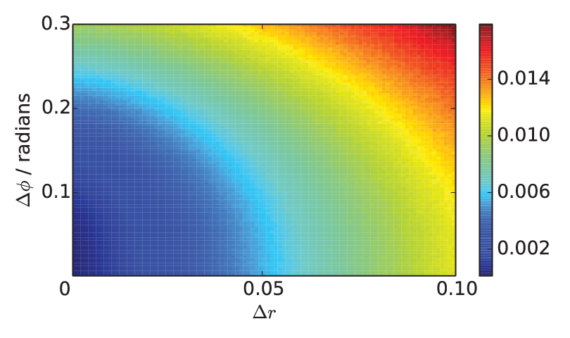
In practice, spatial refocusing is subject to several types of experimental noise. First of all, the ions are not stationary point particles. Their positions fluctuate thermally and quantum mechanically. Second, the amplitudes and phases of each beam in the array may deviate from the prescription. It is unclear whether the interference is robust to these deviations. We first estimate the position fluctuations of the ions. Take a 21 ion chain as example, the ion spacing vary between $1.02\upmu\text{m}$ and $1.78\upmu\text{m}$ with the smallest spacing in the middle of the chain. Among the axial motional modes the center of mass mode has the lowest frequency, about $2\pi\times 1\text{MHz}$ and the corresponding oscillator length is $\sqrt{\hbar/2M\omega_{z}}\approx 5.4\text{nm}$. The other axial modes all have higher frequencies and the oscillator lengths are even smaller. Assuming the Doppler cooling limit, i.e. with temperature given by $k_{B}T=\hbar\Gamma/2$ and the cooling transition linewidth $\Gamma\approx 2\pi\times 20\text{MHz}$, the center of mass mode along $z$ contains on average $\frac{k_{B}T}{\hbar\omega_{z}}\approx 10$ phonons for a trap with $\omega_{z}=2\pi\times 1\text{MHz}$. With these realistic data, exact numerical calculation taking all the axial modes into account shows that for each ion the standard deviation of position ranges from $6.5\text{nm}$ to $10\text{nm}$, at least two orders of magnitude smaller than the inter-ion spacing. So for our purpose here the noise caused by ions’ thermal motion is negligible. For the second problem, since the laser beams superpose linearly to give the final refocused pulse, an arbitrary deviation of the j-th pulse’s amplitude $\delta f(x_{j}-x_{i})$ only add noise $\delta f(x_{j}-x_{i})g(x-x_{j})$ to the final amplitude distribution $G(x-x_{i})$. To consider both strength and phase error of the laser, we allow the deviation $\delta f(x_{j}-x_{i})$ to be a complex number. To quantify the effect of $\delta f(x_{j}-x_{i})$, we parametrize the deviation as follows

where the real numbers $r_{j}$ and $\phi_{j}$ measure respectively the relative amplitude error and phase error of the beam on ion $j$. Each $r_{j}$/$\phi_{j}$ is sampled from the normal distribution with zero mean and standard deviation $\Delta r$/$\Delta\phi$, i.e. $r_{j}\sim\mathcal{N}(0,\sigma^{2}=\Delta r^{2})$ and $\phi_{j}\sim\mathcal{N}(0,\sigma^{2}=\Delta\phi^{2})$. We define the quantity

to measure the difference of actual and ideal intensity distribution. We now do a numerical simulation to investigte the robustness of the interference. We take a 21-ion chain harmonically trapped and try to address the central ion, $i=11$. The ideal target is $G(x_{j}-x_{11})=\delta_{j,11}$. Assume the addressing beams have a Gaussian profile with width the same as the distance between 11-th and 12-th ion. We randomly sample $r_{j}$ and $\phi_{j}$ 5000 times, calculate $\epsilon$ for each sample and plot the average $\bar{\epsilon}$ as a function of $\Delta r$ and $\Delta\phi$, in Fig 4. We found that the interference pattern is pretty robust. For 5% standard amplitude error and 0.2 radians phase error, the average intensity error $\bar{\epsilon}$ is still below 1%. In terms of gate infidelity, we did numerical experiments and found that 1% intensity error induces on the order of $10^{-2}$ ($10^{-3}$) infidelity for two center ions with $n_{\text{corr}}=8$ (edge ions with $n_{\text{corr}}=5$), with every other parameter the same as described in caption of fig 3. For 0.5% intensity error, both infidelities are on the $10^{-3}$ level.

In summary, we have proposed a spatial refocusing technique to achieve effective individual addressing and reduce crosstalk error in a general multi-qubit platform. The scheme is efficient as the crosstalk error decreases exponentially with the number of correction beams, and the cost in the laser power is modest even when the beam width is comparable with the qubit separation. The scheme works universally for any type of quantum gates and can apply to any quantum computational platform.

This work was supported by the NBRPC (973 Program) 2011CBA00300 (2011CBA00302), the IARPA MUSIQC program, the ARO and the AFOSR MURI program, and the DARPA OLE program. We thank Kihwan Kim for helpful discussion.

According to the Toeplitz matrix theory, the general solution to the equation $M_{lj}f_{ji}=\delta_{li}$ has the form $f_{ji}=\sum_{k}c_{k}^{+/-}\left(a_{k}\right){}^{j-i}$ where $c_{k}^{+}$ and $c_{k}^{-}$ are for the regions $j>i$ and $j<i$, respectively. Here $a_{k}$ are the roots of the polynomial $P_{n}(x)=x^{n}\left(1+\sum_{m=1}^{n}\left(1\left/x^{m}\right.+x^{m}\right)\gamma^{m^{2}}\right)$ and $c_{k}^{+/-}$ are coefficients to be determined (the band-width of the matrix $M_{lj}$ is $2n+1$). Our first observation is that the roots come in pairs ($a$ , $1/a$ ) due to the symmetry $x\leftrightarrow 1/x$. Thus $f_{ji}$ is composed of terms like $c_{k}^{+/-}(a_{k})^{j-i}$ decaying (increasing) exponentially with $\left|j-i\right|$ if $a_{k}<1$ ($a_{k}>1$). In the region $j>i$ ($j<i$) , boundary condition at $\left|j-i\right|\rightarrow\infty$ requires $c_{k}=0$ for $a_{k}>1$ ($a_{k}>1$). Note that in the large $\left|j-i\right|$ limit, the $a_{k}$ closest to the unity should dominate since other components die out more quickly. Next we prove that $-\gamma$ (and hence $-1/\gamma$) is a root of $P_{n}(x)$ when $n$ is sufficiently large.

The characteristic quantities of $P_{n}(x)$ are $\gamma$, $\gamma^{4}$, $\gamma^{9}$, …, of which the one closest to the unity is $\gamma$. This leads us to conjecture $(-\gamma)$ is the root of $P_{n}(x)$ closest to $1$ in magnitude. This turns out to be true. Since $\tilde{P}_{n}(x)=P_{n}(x)/x^{n}>0$ when $x>0$, there is no positive root. Let us focus on the interval $[-1,0)$. For $n=1$, $\tilde{P}_{1}(x)=1+\gamma(1/x+x)$ is monotonically decreasing from $\tilde{P}_{1}(-1)=1-2\gamma$ to $\tilde{P}_{1}(0^{-})\rightarrow-\infty$ and there is one root in this interval: $\frac{-1+\sqrt{1-4\gamma^{2}}}{2\gamma}\approx\frac{-1+1-2\gamma^{2}}{2\gamma}=-\gamma$. When increasing $n$ by $1$, we include one more term $Q_{n+1}(x)=\left(1/x^{n+1}+x^{n+1}\right)\gamma^{(n+1)^{2}}$. Due to the small factor $\gamma^{(n+1)^{2}}$, the contribution of $Q_{n+1}$ can be comparable with that of $Q_{n}$ only when $\left|x\right|\lesssim\gamma^{2n+1}$. Since $Q_{n}(0^{-})$ approaches $+\infty$ for even $n$ and $-\infty$ for odd $n$ and $Q_{n}$ is always monotonic on $[-1,0)$, adding one more term always introduces one more turning point in $\tilde{P}_{n}(x)$ and thus adds one more root with magnitude much smaller than the previous roots. Therefore $(-\gamma)$ is the root with the largest magnitude by far on $[-1,0)$. We therefore conclude $f_{ji}\propto(-\gamma)^{|j-i|}$ when $\left|j-i\right|$ is large.

References

- [1] J. P. Home, et.al., Science 325, 1227 (2009); M. Anderlini, et. al., Nature 448, 452 (2007); J. R. Petta, et. al., Science 309, 2180 (2005); M. Steffen, et. al., Science 313, 1423 (2006); L. Isenhower, et. al., Phys. Rev. Lett. 104, 010503 (2010); T. Wilk, et. al., Phys. Rev. Lett. 104, 010502 (2010).
- [2] L. DiCarlo, et. al., Nature 460, 240 (2009); A. Politi, et.al., Science 325, 1221 (2009); E. Lucero, et. al., Nature Physics 8, 719 (2012);
- [3] M. D. Reed, et. al., Nature 482, 382 (2012); P. Schindler, et. al., Science 332, 1059 (2011).
- [4] K. Kim, et. al., Nature 465, 590 (2010); R. Islam, et. al., Nature Communications 2, 377 (2011); J. T. Barreiro, et. al., Nature 470, 486(24 February 2011); B. P. Lanyon, et. al., Science 334, 57 (2011).
- [5] M. A. Nielsen, I. L. Chuang, Quantum Computation and Quantum Information, Cambridge University Press (2000).
- [6] C. Kim, C. Knoernschild, B. Liu, and J. Kim, IEEE J. Sel. Top. Quantum Electron. 13, 322 (2007); C. Knoernschild, et. al., Appl. Phys. Lett. 97, 134101 (2010).
- [7] W. S. Bakr, et. al., Nature 462, 74 (2009); J. F. Sherson, et. al., Nature 467, 68 (2010).
- [8] M. Saffman, Opt. Lett. 29, 1016 (2004).
- [9] G. S. Agarwal and K. T. Kapale, J. Phys. B 39, 3437 (2006); J. Cho, Phys. Rev. Lett. 99, 020502 (2007); D. D. Yavuz and N. A. Proite, Phys. Rev. A 76, 041802(R) (2007); A. V. Gorshkov, L. Jiang, M. Greiner, P. Zoller, and M. D. Lukin , Phys. Rev. Lett. 100, 093005 (2008); D. Viscor, et. al., Phys. Rev. A 86, 063409 (2012);
- [10] J. A. Miles, Z. J. Simmons and D. D. Yavuz, Phys. Rev. X 3, 031014 (2013)
- [11] C. Weitenberg, et. al., Nature 471, 319 (2011).
- [12] U. Haeberlen, High Resolution NMR in Solids, Advances in Magnetic Resonance Series, Supplement 1 (Academic Press, New York, 1976).
- [13] See H. K. Ng, D. A. Lidar, J. Preskill, Phys. Rev. A 84, 012305 (2011) and references therein.
- [14] K. R. Brown, A. W. Harrow, and I. L. Chuang, Phys. Rev. A 70, 052318 (2004).
- [15] Y. Tomita, J. T. Merrill and K. R. Brown, New J. Phys. 12 015002 (2010).
- [16] W. F. Trench, J. Soc. Indust. Appl. Math., 12, 515, 1964.
- [17] S. Korenblit et al., New J. Phys. 14, 095024 (2012).
- [18] S.-L. Zhu, C. Monroe, L.-M. Duan, Phys. Rev. Lett. 97, 050505 (2006).
- [19] S.-L. Zhu, C. Monroe, L.-M. Duan, Europhys. Lett. 73, 485 (2006).
- [20] D.F.V James, Appl. Phys. B 66, 181 (1998).
- [21] G.-D. Lin et al., Europhys. Lett. 86, 60004 (2009).
- [22] J. D. Siverns, et. al., New J. Phys. 14, 085009 (2012); J. M. Amini, et. al.,New J. Phys. 12, 033031 (2010).
- [23] M. Saffman, T. G. Walker and K. Mølmer, Rev. Mod. Phys. 82, 2313 (2010).
- [24] R. Dumke, et. al., Phys. Rev. Lett., 89, 097903 (2002); S. Bergamini, et. al., JOSA B 21, 1889 (2004).