跳到论文正文
W Papers独立论文阅读器 arXiv:1305.2651 论文正文 计算阅读时间 · 0%
引用这篇论文根据当前论文元数据生成,正式投稿前建议核对。


License: arXiv.org perpetual non-exclusive license
arXiv:1305.2651v3 [math.OC] 23 Sep 2013

Stable Hierarchical Model Predictive Control Using an Inner Loop Reference Model and λ\lambda-Contractive Terminal Constraint Sets

Chris Vermillion Address: Altaeros Energies, Boston, MA 02110 (e-mail: chris.vermillion@altaerosenergies.com)    Amor Menezes Address: California Institute for Quantitative Biosciences, University of California, Berkeley, Berkeley, CA 94704 (e-mail: amenezes@berkeley.edu)    Ilya Kolmanovsky Address: Department of Aerospace Engineering, University of Michigan, Ann Arbor, MI 48109 (e-mail: ilya@umich.edu)
Abstract

This paper presents a hierarchical model predictive control (MPC) framework that is presented in Vermillion, Menezes, Kolmanovsky (2011) and Vermillion, Menezes, Kolmanovsky (2013), along with proofs that were omitted in the aforementioned works. The method described in this paper differs significantly from previous approaches to guaranteeing overall stability, which have relied upon a multi-rate framework where the inner loop (low level) is updated at a faster rate than the outer loop (high level), and the inner loop must reach a steady-state within each outer loop time step. In contrast, the method proposed in this paper is aimed at stabilizing the origin of an error system characterized by the difference between the inner loop state and the state specified by a full-order reference model. This makes the method applicable to systems with reduced levels of time scale separation. This paper reviews the fundamental results of Vermillion, Menezes, Kolmanovsky (2011) and Vermillion, Menezes, Kolmanovsky (2013) and presents proofs that were omitted due to space limitations.

Keywords: 
Model predictive control, Hierarchical control, Control of constrained systems, Decentralization.

1 Introduction

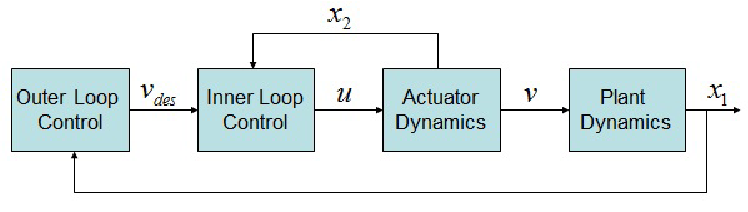
This paper focuses on a two-layer inner loop/outer loop hierarchical control structure where the ultimate objective is to stabilize the overall system. The actuator and plant represent a cascade, depicted in Fig. 1, wherein an actuator output, denoted by vv, characterizes an overall force, moment, or generalized effect produced by the actuators, and is referred to as a virtual control input. In the hierarchical control strategy, an outer loop controller sets a desired value for this virtual control input, denoted by vd​e​sv_{des}, and it is the responsibility of the inner loop to generate control inputs uu that drive vv close to vd​e​sv_{des}.

Refer to caption
Figure 1: Block diagram of the actuator/plant cascade considered in this work.

This control approach is employed in a number of automotive, aerospace, and marine applications, such as Luo et. al. (2004), Luo et. al. (2005), Luo et. al. (2007), Tjonnas, Johansen (2007), and Vermillion et. al. (2007). Hierarchical control has become commonplace in industrial applications, as it offers two key advantages over its centralized counterpart:

  1. 1.

    Plug-and-play integration of new design features (for example, a new inner loop) without requiring a complete system redesign;

  2. 2.

    Reduction in overall computational complexity, in terms of the number of inputs and/or states considered by each controller.

The use of MPC for constrained hierarchical control has been a natural choice in instances when constraint satisfaction was critical and/or multiple control objectives were traded off. Only recently, however, has an effort been made to provide theoretical stability guarantees for the hierarchical system. In many recent papers, including Falcone et. al. (2008), Scattolini, Colaneri (2007), Scattolini et. al. (2008), Scattolini (2009), and Picasso et. al. (2010), the inner loop is updated at a faster rate than the outer loop, and the inner loop is designed to reach a steady-state, wherein v=vd​e​sv=v_{des}, within a single outer loop time step. This strategy represents an effective way of guaranteeing stability under large time-scale separation, but numerous systems, including those described in Luo et. al. (2004), Luo et. al. (2005), and Luo et. al. (2007) (which address a flight control application), and Vermillion et. al. (2007), Vermillion et. al. (2009), and Vermillion et. al. (2011) (which address a thermal management system), do not exhibit such a demonstrable time scale separation.

Our approach differs from that of Scattolini, Colaneri (2007), Scattolini et. al. (2008), and Picasso et. al. (2010) in that it drives the inner loop states to those of a reference model rather than to the steady state values corresponding to vd​e​sv_{des}. Our stability formulation relies on λ\lambda-contractive terminal constraint sets for the outer and inner loop, in addition to rate-like constraints that ensure that the optimized MPC trajectories do not vary too much from one instant to the next. The contractive nature of the terminal constraint allows MPC-optimized control input trajectories to vary from one time step and the next.

The work presented in this paper is an extension of an original IFAC conference paper (Vermillion, Menezes, Kolmanovsky (2011)) and builds upon it through two key mechanisms:

  • •

    Allowance for inexact (approximate) inner loop reference model matching;

  • •

    Greater flexibility in the decay of contraction rates within the MPC optimization.

2 Problem Statement

In this paper, we consider two interconnected systems, as depicted in Fig. 3, whose dynamics in discrete time are given by:

x1​(k+1)\displaystyle x_{1}(k+1) =\displaystyle= A1​x1​(k)+B1​v​(k),\displaystyle A_{1}x_{1}(k)+B_{1}v(k),
x2​(k+1)\displaystyle x_{2}(k+1) =\displaystyle= A2​x2​(k)+B2​u​(k),\displaystyle A_{2}x_{2}(k)+B_{2}u(k), (1)
v⁡(k)\displaystyle v(k) =\displaystyle= C​x2​(k),\displaystyle Cx_{2}(k),

where v∈ℝqv\in\mathbb{R}^{q} represents the virtual control input, x1∈ℝn1x_{1}\in\mathbb{R}^{n_{1}} represents the plant states, which are driven by the virtual control input, vv, whereas x2∈ℝn2x_{2}\in\mathbb{R}^{n_{2}} represents the actuator states, which are driven by the real control inputs, u∈ℝpu\in\mathbb{R}^{p}, where p≥qp\geq q. The control inputs, uu are subject to a saturation constraint set UU, such that u⁡(k)∈Uu(k)\in U at every time instant. We assume that:

  • •

    Assumption 1: The pair (A1,B1)(A_{1},B_{1}) is stabilizable.

  • •

    Assumption 2: The pair (A2,B2)(A_{2},B_{2}) is controllable.

  • •

    Assumption 3: Without loss of generality, the actuator dynamics of (1) are written in block controllable canonical form (CCF) described in Luenberger (1967).

The assumption of stabilizability is clearly essential to any problem whose objective is stabilization of the origin. The stronger assumption of inner loop controllability (Assumption 2) allows us to generate an inner loop error system and control law that appropriately places all of the poles of the closed inner loop to satisfy the reference model specifications.

3 Control Design Formulation

Our approach relies on the design of an inner loop reference model, which describes the ideal input-output behavior from vd​e​sv_{des} to vv. We will proceed to derive an error system describing the difference between the inner loop and reference model states, and we will show how closed-form control laws can be used to achieve exact or sufficiently accurate reference model matching near the origin of this system, ultimately resulting in local stability of the overall system. MPC is used to enlarge the region of attraction of the overall system to include states under which the closed-form control laws hit saturation constraints.

The specific control algorithm incorporates both outer and inner loop terminal constraint sets, wherein closed-form control laws are used to achieve reference model matching (or approximate matching) behavior. Farther from the origins of the outer and inner loops, MPC is used to drive the system into these constraint sets, explicitly accounting for saturation constraints.

3.1 Reference Model Design and Assumptions

This reference model is given by:

xf​(k+1)\displaystyle x_{f}(k+1) =\displaystyle= Af​xf​(k)+Bf​vd​e​s​(k),\displaystyle A_{f}x_{f}(k)+B_{f}v_{des}(k), (2)
vd​e​sf​(k)\displaystyle v_{des}^{f}(k) =\displaystyle= C​xf​(k),\displaystyle Cx_{f}(k),

where xf∈ℝn2x_{f}\in\mathbb{R}^{n_{2}}, vd​e​s∈ℝqv_{des}\in\mathbb{R}^{q}, and vd​e​sf∈ℝqv_{des}^{f}\in\mathbb{R}^{q}. We assume that:

  • •

    Assumption 4: The reference model is stable, i.e., ∥λ¯i(Af))∥<1,∀i\|\bar{\lambda}_{i}(A_{f}))\|<1,\forall i (λ¯i\bar{\lambda}_{i} represents the it​hi^{th} eigenvalue of AfA_{f});

  • •

    Assumption 5: The reference model does not share any zeros with unstable poles of A1A_{1}.

Because Assumptions 4 and 5 are on the reference model, which is freely chosen by the control system designer, they do not restrict the applicability of the proposed control design.

We use the reference model to analyze the closed-loop behavior of the inner loop through the following error system:

x~​(k+1)\displaystyle\tilde{x}(k+1) =\displaystyle= A2​x~​(k)+(A2−Af)​xf​(k)+B2​u​(k)\displaystyle A_{2}\tilde{x}(k)+(A_{2}-A_{f})x_{f}(k)+B_{2}u(k) (3)
−Bf​vd​e​s​(k),\displaystyle-B_{f}v_{des}(k),
v~​(k)\displaystyle\tilde{v}(k) =\displaystyle= C​x~​(k),\displaystyle C\tilde{x}(k),

where x~​(k)=x2​(k)−xf​(k)\tilde{x}(k)=x_{2}(k)-x_{f}(k) and it follows that v~​(k)=v⁡(k)−vd​e​sf​(k)\tilde{v}(k)=v(k)-v_{des}^{f}(k). For notational convenience throughout the paper, because the reference model is embedded in the outer loop, we will introduce the augmented outer loop state, x1a​u​g≜[x1TxfT]Tx_{1}^{aug}\triangleq\left[\begin{array}[]{cc}x_{1}^{T}&x_{f}^{T}\end{array}\right]^{T}, which results in augmented outer loop dynamics given by:

x1a​u​g​(k+1)\displaystyle x_{1}^{aug}(k+1) =\displaystyle= A1a​u​g​x1a​u​g​(k)+B1a​u​g​v~​(k)\displaystyle A_{1}^{aug}x_{1}^{aug}(k)+B_{1}^{aug}\tilde{v}(k) (4)
+Bfa​u​g​vd​e​s​(k)\displaystyle+B_{f}^{aug}v_{des}(k)

where:

A1a​u​g\displaystyle A_{1}^{aug} =\displaystyle= [A1B1​C0Af],\displaystyle\left[\begin{array}[]{cc}A_{1}&B_{1}C\\ 0&A_{f}\end{array}\right],
B1a​u​g\displaystyle B_{1}^{aug} =\displaystyle= [B1T0]T,\displaystyle\left[\begin{array}[]{cc}B_{1}^{T}&0\end{array}\right]^{T},
Bfa​u​g\displaystyle B_{f}^{aug} =\displaystyle= [0BfT]T.\displaystyle\left[\begin{array}[]{cc}0&B_{f}^{T}\end{array}\right]^{T}.

3.2 Model Predictive Control Framework

An MPC optimization is carried out whenever the outer or inner loop states are outside of predetermined λ\lambda-contractive terminal constraint sets G1G_{1} and G2G_{2} respectively. A closed-form terminal control law is active once the inner and outer loop states have reached the terminal sets. The block diagram of the closed-loop system when MPC is active is given in Fig. 2, whereas the closed-loop system under closed-form terminal control laws conforms to the block diagram of Fig. 3.

Whenever the MPC optimization is carried out, an optimal control trajectory is computed for an NN step prediction horizon, along with a corresponding state trajectory. The outer loop virtual control and state trajectories are given by:

𝐯𝐝𝐞𝐬​(k)\displaystyle\mathbf{v_{des}}(k) =\displaystyle= [𝐯𝐝𝐞𝐬​(k|k)…𝐯𝐝𝐞𝐬​(k+N−1|k)],\displaystyle\left[\begin{array}[]{ccc}\mathbf{v_{des}}(k|k)&\ldots&\mathbf{v_{des}}(k+N-1|k)\end{array}\right],
𝐱𝟏𝐚𝐮𝐠​(k)\displaystyle\mathbf{x_{1}^{aug}}(k) =\displaystyle= [𝐱𝟏𝐚𝐮𝐠​(k|k)…𝐱𝟏𝐚𝐮𝐠​(k+N|k)].\displaystyle\left[\begin{array}[]{ccc}\mathbf{x_{1}^{aug}}(k|k)&\ldots&\mathbf{x_{1}^{aug}}(k+N|k)\end{array}\right].

The inner loop control and state trajectories are given by:

𝐮⁡(k)\displaystyle\mathbf{u}(k) =\displaystyle= [𝐮⁡(k|k)…𝐮⁡(k+N−1|k)],\displaystyle\left[\begin{array}[]{ccc}\mathbf{u}(k|k)&\ldots&\mathbf{u}(k+N-1|k)\end{array}\right],
𝐱~​(k)\displaystyle\mathbf{\tilde{x}}(k) =\displaystyle= [𝐱~​(k|k)…𝐱~​(k+N|k)].\displaystyle\left[\begin{array}[]{ccc}\mathbf{\tilde{x}}(k|k)&\ldots&\mathbf{\tilde{x}}(k+N|k)\end{array}\right].

The notation (i|k)(i|k) denotes the chosen/predicted value of a variable at step ii when the optimization is carried out at time kk (k≤ik\leq i).

Refer to caption
Figure 2: Block diagram of the hierarchical control strategy that is implemented when model predictive control is active. In this scenario, N-step predictions of interconnection variables (shown in bold) are passed between the inner and outer loop optimizations.
Refer to caption
Figure 3: Block diagram of the hierarchical control strategy that is implemented under terminal control laws.

The mathematical description of the outer loop control law is:

vd​e​s​(k)\displaystyle v_{des}(k) =\displaystyle= {−K1​x1a​u​g​(k)ifx1a​u​g(k)∈G1,x~(k)∈G2,𝐯𝐝𝐞𝐬𝐨​(k|k),otherwise\displaystyle\left\{\begin{array}[]{ccccc}-K_{1}x_{1}^{aug}(k)&\text{if}&x_{1}^{aug}(k)\in G_{1},\tilde{x}(k)\in G_{2},\\ \mathbf{v_{des}^{o}}(k|k)&,&\text{otherwise}\end{array}\right.

Here, K1K_{1} is the terminal control gain and 𝐯d​e​so​(k)\mathbf{v}_{des}^{o}(k) is the optimized control input sequence from the outer loop MPC optimization, given by:

𝐯𝐝𝐞𝐬𝐨​(k)=arg⁡min𝐯𝐝𝐞𝐬∈𝐕𝐝𝐞𝐬​J1​(𝐯𝐝𝐞𝐬​(k)|x1a​u​g​(k),𝐯~​(k−1)),\mathbf{v_{des}^{o}}(k)=\arg\underset{\mathbf{v_{des}}\in\mathbf{V_{des}}}{\min}J_{1}(\mathbf{v_{des}}(k)|x_{1}^{aug}(k),\mathbf{\tilde{v}}(k-1)), (23)

subject to the dynamics of (4) and constraints:

𝐱𝟏𝐚𝐮𝐠​(k+N−1|k)\displaystyle\mathbf{x_{1}^{aug}}(k+N-1|k) ∈\displaystyle\in G1,\displaystyle G_{1},
𝐱𝟏𝐚𝐮𝐠​(k+N|k)\displaystyle\mathbf{x_{1}^{aug}}(k+N|k) ∈\displaystyle\in λ1​G1,\displaystyle\lambda_{1}G_{1}, (24)
‖𝐯𝐝𝐞𝐬​(k+i|k)−𝐯𝐝𝐞𝐬𝐨​(k+i|k−1)‖\displaystyle\|\mathbf{v_{des}}(k+i|k)-\mathbf{v_{des}^{o}}(k+i|k-1)\| ≤\displaystyle\leq (δvd​e​sm​a​x)​βmin⁡(k,N1∗),\displaystyle(\delta_{v_{des}}^{max})\beta^{\min(k,N_{1}^{*})},
i=0​…​N−2,\displaystyle i=0\ldots N-2,

and cost function:

J1​(𝐯𝐝𝐞𝐬​(k)|x1a​u​g​(k),𝐯~​(k−1))\displaystyle J_{1}(\mathbf{v_{des}}(k)|x_{1}^{aug}(k),\mathbf{\tilde{v}}(k-1)) =\displaystyle= ∑i=kk+N−1g1​(𝐱𝟏𝐚𝐮𝐠​(i|k)CLOSE,\displaystyle\sum_{i=k}^{k+N-1}g_{1}(\mathbf{x_{1}^{aug}}(i|k), (25)
OPEN𝐯𝐝𝐞𝐬​(i|k)).\displaystyle\mathbf{v_{des}}(i|k)).

Here, λ1\lambda_{1}, δvd​e​sm​a​x\delta_{v_{des}}^{max}, β\beta, and N1∗N_{1}^{*} are design parameters, which are summarized in Table 1. 𝐕𝐝𝐞𝐬\mathbf{V_{des}} is the set of all feasible 𝐯𝐝𝐞𝐬\mathbf{v_{des}} trajectories. For the results in this paper, there are no restrictions to the form of the stage cost, g1​(𝐱𝟏𝐚𝐮𝐠​(i|k),𝐯𝐝𝐞𝐬​(i|k))g_{1}(\mathbf{x_{1}^{aug}}(i|k),\mathbf{v_{des}}(i|k)). The mathematical description of the inner loop control law is:

u⁡(k)\displaystyle u(k) =\displaystyle= {ut​(k)i​fx1a​u​g​(k)∈G1,x~​(k)∈G2𝐮𝐨​(k|k),o​t​h​e​r​w​i​s​e\displaystyle\left\{\begin{array}[]{ccccc}u_{t}(k)&if&x_{1}^{aug}(k)\in G_{1},\tilde{x}(k)\in G_{2}\\ \mathbf{u^{o}}(k|k)&,&otherwise\end{array}\right.

where

ut​(k)=K21​vd​e​s​(k)−K22​x2​(k).u_{t}(k)=K_{21}v_{des}(k)-K_{22}x_{2}(k). (28)

Here, 𝐮𝐨​(k)\mathbf{u^{o}}(k) is the optimized control input sequence from the inner loop MPC optimization, given by:

𝐮𝐨​(k)=arg⁡min𝐮⁡(k)∈𝐔​J2​(𝐮⁡(k)|x~​(k),𝐱𝐟​(k)),\mathbf{u^{o}}(k)=\arg\underset{\mathbf{u}(k)\in\mathbf{U}}{\min}J_{2}(\mathbf{u}(k)|\tilde{x}(k),\mathbf{x_{f}}(k)), (29)

subject to the dynamics of (3) and constraints:

𝐱~​(k+N|k)\displaystyle\mathbf{\tilde{x}}(k+N|k) ∈\displaystyle\in λ2​G2,\displaystyle\lambda_{2}G_{2},
‖𝐮⁡(k+i|k)−𝐮𝐨​(k+i|k−1)‖\displaystyle\|\mathbf{u}(k+i|k)-\mathbf{u^{o}}(k+i|k-1)\| ≤\displaystyle\leq (δum​a​x)​βmin⁡(k,N2∗),\displaystyle(\delta_{u}^{max})\beta^{\min(k,N_{2}^{*})}, (30)
i=0​…​N−2\displaystyle i=0\ldots N-2
𝐮⁡(k+i|k)\displaystyle\mathbf{u}(k+i|k) ∈\displaystyle\in U,i=0​…​N−1,\displaystyle U,i=0\ldots N-1,

where UU reflects the actuator saturation limits of uu and 𝐔\mathbf{U} is the set of all feasible control input 𝐮\mathbf{u} trajectories. The inner loop cost function is given by:

J2​(𝐮⁡(k)|x~​(k),𝐱𝐟​(k))=∑i=kk+N−1g2​(𝐱~​(i|k),𝐮⁡(i|k)).J_{2}(\mathbf{u}(k)|\tilde{x}(k),\mathbf{x_{f}}(k))=\sum_{i=k}^{k+N-1}g_{2}(\mathbf{\tilde{x}}(i|k),\mathbf{u}(i|k)). (31)

Here, λ2\lambda_{2}, δum​a​x\delta_{u}^{max}, β\beta, and N2∗N_{2}^{*} are design parameters, which are summarized in Table 1. As with the outer loop, there are no restrictions to the form of the stage cost, g2​(𝐱~​(i|k),𝐮⁡(i|k))g_{2}(\mathbf{\tilde{x}}(i|k),\mathbf{u}(i|k)).

The terms βmin⁡(k,N1∗)\beta^{\min(k,N_{1}^{*})} and βmin⁡(k,N2∗)\beta^{\min(k,N_{2}^{*})} impose the requirement that trajectories 𝐯𝐝𝐞𝐬​(k)\mathbf{v_{des}}(k) and 𝐮⁡(k)\mathbf{u}(k) calculated at any two subsequent time steps must be sufficiently close to each other, and that the required proximity of trajectories decrease over time, until k=N1∗k=N_{1}^{*} and k=N2∗k=N_{2}^{*}, respectively. Formulas for the required values for N1∗N_{1}^{*} and N2∗N_{2}^{*} are given in the proof of Proposition 10; required values depend on the contraction rates λ1\lambda_{1} and λ2\lambda_{2}, system dynamics, horizon length (NN), and β\beta.

Key MPC design parameters, including those that are essential for our stability formulation, are provided in Table 1. Fig. 4 provides a graphical depiction of the sequence of operations that occur in a single time instant when MPC is active.

Refer to caption
Figure 4: Sequence of operations when MPC is active, including the physical locations where the operations occur.

Computationally, the outer loop MPC must consider n1+n2n_{1}+n_{2} states and qq control inputs, whereas the inner loop must consider n2n_{2} states and pp control inputs. Both optimizations are individually computationally simpler than their centralized counterparts, which must consider n1+n2n_{1}+n_{2} states and pp control inputs. The resulting computational simplification can be especially significant when the algorithm is applied to systems with complex outer loops (n1>>n2n_{1}>>n_{2}) and several actuators for a given virtual control (p>>qp>>q), which is commonplace in industry.

Table 1: Key MPC Design Parameters
Parameter Description
G1G_{1} outer loop terminal constraint set
G2G_{2} inner loop terminal constraint set
K1K_{1} outer terminal control gain matrix
K21,K22K_{21},K_{22} inner terminal control gain matrices
λ1\lambda_{1} outer contraction rate (<1<1)
λ2\lambda_{2} inner contraction rate (<1<1)
δvd​e​sm​a​x\delta_{v_{des}}^{max} rate-like constraint on outer loop MPC
δum​a​x\delta_{u}^{max} rate-like constraint on inner loop MPC
β\beta any scalar that is <1<1
N1∗N_{1}^{*} maximum steps until convergence to G1G_{1}
N2∗N_{2}^{*} maximum steps until convergence to G2G_{2}

4 Deriving Terminal Control Laws and λ\lambda-Contractive Terminal Constraint Sets

In this section, we will first derive control laws that, in the absence of constraints, will lead to overall system stability. Having derived these control laws, we will then show that there exist λ\lambda- contractive sets G1G_{1} and G2G_{2}, as described in Lin, Antsaklis (2004), such that once x1a​u​gx_{1}^{aug} and x~\tilde{x} enter G1,G2G_{1},G_{2}, they remain there (and in fact are driven further into the sets at the next instant).

We consider two options for inner loop terminal control design, namely:

  • •

    Exact reference model matching - We design the inner loop control law such that x~​(k+1)=Af​x~​(k)\tilde{x}(k+1)=A_{f}\tilde{x}(k), which guarantees that v⁡(k)v(k) asymptotically tracks vd​e​sf​(k)v_{des}^{f}(k).

  • •

    Approximate reference model matching - The inner loop control law is designed such that the closed inner loop is stable and a small gain condition is satisfied.

4.1 Terminal Control Law Design with Exact Reference Model Matching

In the case of exact reference model matching, in order to derive a model-matching controller, we assume that the reference model is cast in a specific form that is compatible with the actuator dynamics; specifically, we assume that:

  • •

    Assumption 6. AfA_{f} in (2) is written in the same block CCF as A2A_{2} (as described in Luenberger (1967)).

  • •

    Assumption 7. Taking R2R_{2} and RfR_{f} as the set of rows of B2B_{2} and BfB_{f}, respectively, that contain nonzero entries (which also correspond to the full rows of A2A_{2} and AfA_{f}), we assume that Rf⊂R2R_{f}\subset R_{2}, i.e., each nonzero row of BfB_{f} is also a nonzero row of B2B_{2}.

These assumptions, in conjunction with Assumptions 1-5, place restrictions on AfA_{f} and BfB_{f} that ensure that a stabilizing, reference model-matching inner loop control law can be designed. In particular,it is possible to design outer and inner loop terminal control laws with desirable properties, according to the following proposition:

Proposition 1

(Terminal control laws for exact matching): Given that Assumptions 1-7 hold, there exist control laws vd​e​s​(k)=−K1​x1a​u​g​(k)v_{des}(k)=-K_{1}x_{1}^{aug}(k) and u⁡(k)=K21​vd​e​s​(k)−K22​x2​(k)u(k)=K_{21}v_{des}(k)-K_{22}x_{2}(k) which, when substituted into (4) and (3), yield:

x1a​u​g​(k+1)\displaystyle x_{1}^{aug}(k+1) =\displaystyle= (A1a​u​g−B1a​u​g​K1)​x1a​u​g​(k)\displaystyle(A_{1}^{aug}-B_{1}^{aug}K_{1})x_{1}^{aug}(k) (32)
+B1a​u​g​v~​(k),\displaystyle+B_{1}^{aug}\tilde{v}(k),
x~​(k+1)\displaystyle\tilde{x}(k+1) =\displaystyle= Af​x~​(k),\displaystyle A_{f}\tilde{x}(k),

where ∥λ¯i(A1a​u​g−B1a​u​gK1))∥<1,∀i\|\bar{\lambda}_{i}(A_{1}^{aug}-B_{1}^{aug}K_{1}))\|<1,\forall i, and render the origin of the overall system, x1a​u​g=0,x~=0x_{1}^{aug}=0,\tilde{x}=0, asymptotically stable.

{@proof}

[Proof.] Since the pair (A1,B1)(A_{1},B_{1}) is controllable and the reference model does not share zeros with unstable poles of A1A_{1}, it follows that the pair (A1a​u​g,B1a​u​g)(A_{1}^{aug},B_{1}^{aug}) is stabilizable. Thus, K1K_{1} can be designed to ensure that ∥λ¯i(A1a​u​g−B1a​u​gK1))∥<1,∀i\|\bar{\lambda}_{i}(A_{1}^{aug}-B_{1}^{aug}K_{1}))\|<1,\forall i.

To show the second part of the proposition, recall that the inner loop dynamics are expressed in (3) by:

x~​(k+1)=A2​x~​(k)+(A2−Af)​xf​(k)+B2​u​(k)−Bf​vd​e​s​(k).\tilde{x}(k+1)=A_{2}\tilde{x}(k)+(A_{2}-A_{f})x_{f}(k)+B_{2}u(k)-B_{f}v_{des}(k). (33)

It follows from the block CCF of A2A_{2}, B2B_{2}, in conjunction with Assumptions 6 and 7 (which impose a suitable block CCF structure on AfA_{f} and BfB_{f}), that we can choose K21K_{21} and K22K_{22} to satisfy:

B2​K21\displaystyle B_{2}K_{21} =\displaystyle= Bf,\displaystyle B_{f}, (34)
B2​K22\displaystyle B_{2}K_{22} =\displaystyle= A2−Af,\displaystyle A_{2}-A_{f},

which, when substituted into the inner loop dynamics, yields:

x~​(k+1)=Af​x~​(k).\tilde{x}(k+1)=A_{f}\tilde{x}(k). (35)

To see this, let R2R_{2} be the indices corresponding to the nonzero rows of B2B_{2}, and let RfR_{f} be the indices corresponding to the nonzero rows of BfB_{f}. Because Assumption 7 requires that that Rf⊆R2R_{f}\subseteq R_{2}, it possible to achieve B2​K21=BfB_{2}K_{21}=B_{f}. Furthermore, let ii represent any zero row of B2B_{2} (and also BfB_{f}). It follows from block CCF (imposed by Assumption 6) and Assumption 7 that A2​i​j=Af​i​j​∀jA_{2ij}=A_{fij}\forall j, making it possible to achieve B2​K22=A2−AfB_{2}K_{22}=A_{2}-A_{f}.

Because ∥λ¯i(A1a​u​g−B1a​u​gK1))∥<1,∀i\|\bar{\lambda}_{i}(A_{1}^{aug}-B_{1}^{aug}K_{1}))\|<1,\forall i and ∥λ¯i(Af))∥<1,∀i\|\bar{\lambda}_{i}(A_{f}))\|<1,\forall i, it follows that both the closed inner and outer loops (32) are input-to-state stable (ISS) under the aforementioned control laws. For small gain analysis, it is convenient to recast the system block diagram of Fig. 3 in the nonminimal representation of Fig. 5, where offsetting copies of the reference model are embedded in both the inner and outer loops. Closed outer loop stability guarantees a finite l2l_{2} gain, γ1\gamma_{1}, from v~\tilde{v} to vd​e​sv_{des}, and exact inner loop reference model matching guarantees an l2l_{2} gain of γ2=0\gamma_{2}=0, from vd​e​sv_{des} to v~\tilde{v}. Therefore, the small gain condition, γ1​γ2<1\gamma_{1}\gamma_{2}<1, is satisfied, and in conjunction with outer and inner loop ISS, this proves asymptotic stability of x1a​u​g=0,x~=0x_{1}^{aug}=0,\tilde{x}=0.

□\Box

Refer to caption
Figure 5: Block diagram of the hierarchical control strategy under terminal control laws, rearranged for analysis purposes.

4.2 Terminal Control Law Design with Inexact Reference Model Matching and Small Gain Condition

For many systems, such as non-minimum phase systems and high-order, high relative degree systems, exact reference model matching is unrealistic. Exact matching is not essential, however, as shown in the following Proposition:

Proposition 2

(Terminal control laws for inexact matching): Given that Assumptions 1-5 hold, there exist control laws vd​e​s​(k)=−K1​x1a​u​g​(k)v_{des}(k)=-K_{1}x_{1}^{aug}(k) and u⁡(k)=K21​vd​e​s​(k)−K22​x2​(k)u(k)=K_{21}v_{des}(k)-K_{22}x_{2}(k) which, when substituted into (4) and (3), yield:

x1a​u​g​(k+1)\displaystyle x_{1}^{aug}(k+1) =\displaystyle= (A1a​u​g−B1a​u​g​K1)​x1a​u​g​(k)+B1a​u​g​v~​(k),\displaystyle(A_{1}^{aug}-B_{1}^{aug}K_{1})x_{1}^{aug}(k)+B_{1}^{aug}\tilde{v}(k),
x~​(k+1)\displaystyle\tilde{x}(k+1) =\displaystyle= (A2−B2​K22)​x~​(k)\displaystyle(A_{2}-B_{2}K_{22})\tilde{x}(k) (36)
+(A2−Af−B2​K22)​xf​(k)\displaystyle+(A_{2}-A_{f}-B_{2}K_{22})x_{f}(k)
+(B2​K21−Bf)​vd​e​s​(k),\displaystyle+(B_{2}K_{21}-B_{f})v_{des}(k),

where ∥λ¯i(A1a​u​g−B1a​u​gK1))∥<1,∀i\|\bar{\lambda}_{i}(A_{1}^{aug}-B_{1}^{aug}K_{1}))\|<1,\forall i and ∥λ¯i(A2−B2K22))∥<1,∀i\|\bar{\lambda}_{i}(A_{2}-B_{2}K_{22}))\|<1,\forall i. Furthermore, suppose that K1K_{1}, K21K_{21}, and K22K_{22} are designed so that the l2l_{2} gains from v~\tilde{v} to vd​e​sv_{des} and vd​e​sv_{des} to v~\tilde{v}, denoted γ1\gamma_{1} and γ2\gamma_{2}, respectively, satisfy the small gain condition, γ1​γ2<1\gamma_{1}\gamma_{2}<1. Then the origin of the overall system, x1a​u​g=0,x~=0x_{1}^{aug}=0,\tilde{x}=0, is asymptotically stable.

{@proof}

[Proof.] Since the pair (A1,B1)(A_{1},B_{1}) is controllable and the reference model does not share zeros with unstable poles of A1A_{1}, it follows that the pair (A1a​u​g,B1a​u​g)(A_{1}^{aug},B_{1}^{aug}) is stabilizable. Thus, K1K_{1} can be designed to ensure that ∥λ¯i(A1a​u​g−B1a​u​gK1))∥<0,∀i\|\bar{\lambda}_{i}(A_{1}^{aug}-B_{1}^{aug}K_{1}))\|<0,\forall i. From Assumption 2, the pair (A2,B2A_{2},B_{2}) is controllable, and therefore there exists K2K_{2} such that ∥λ¯i(A2−B2K2))∥<0,∀i\|\bar{\lambda}_{i}(A_{2}-B_{2}K_{2}))\|<0,\forall i. Thus, both the inner and outer closed-loop dynamics of (36), are input-to-state stable (ISS). By the hypotheses of Proposition 2, the small gain condition, i.e., γ1​γ2<1\gamma_{1}\gamma_{2}<1, is satisfied. Together with ISS, this proves asymptotic stability of x1a​u​g=0,x~=0x_{1}^{aug}=0,\tilde{x}=0.

□\Box

Since ∥λ¯i(A1a​u​g−B1a​u​gK1))∥<1,∀i\|\bar{\lambda}_{i}(A_{1}^{aug}-B_{1}^{aug}K_{1}))\|<1,\forall i and ∥λ¯i(A2−B2K22))∥<1,∀i\|\bar{\lambda}_{i}(A_{2}-B_{2}K_{22}))\|<1,\forall i it follows (Scattolini, Colaneri (2007)) that there exist quadratic Lyapunov functions, V⁡(x1a​u​g)=x1a​u​g,T​Q​x1a​u​gV(x_{1}^{aug})=x_{1}^{aug,T}Qx_{1}^{aug} and V⁡(x~)=x~T​P​x~V(\tilde{x})=\tilde{x}^{T}P\tilde{x}, where QQ and PP are positive definite symmetric matrices, such that when vd​e​s​(k)=−K1​x1a​u​g​(k)v_{des}(k)=-K_{1}x_{1}^{aug}(k) and u⁡(k)=K21​vd​e​s​(k)−K22​x2​(k)u(k)=K_{21}v_{des}(k)-K_{22}x_{2}(k):

V1​(x1a​u​g​(k+1))−V1​(x1a​u​g​(k))\displaystyle V_{1}(x_{1}^{aug}(k+1))-V_{1}(x_{1}^{aug}(k)) <\displaystyle< −α1​V1​(x1a​u​g​(k))\displaystyle-\alpha_{1}V_{1}(x_{1}^{aug}(k)) (37)
+γ¯1​‖v~​(k)‖2,\displaystyle+\bar{\gamma}_{1}\|\tilde{v}(k)\|^{2},
V2​(x~​(k+1))−V2​(x~​(k))\displaystyle V_{2}(\tilde{x}(k+1))-V_{2}(\tilde{x}(k)) <\displaystyle< −α2​V2​(x~​(k))\displaystyle-\alpha_{2}V_{2}(\tilde{x}(k)) (38)
+γ¯21​‖vd​e​s​(k)‖2+γ¯22​‖xf​(k)‖2.\displaystyle+\bar{\gamma}_{21}\|v_{des}(k)\|^{2}+\bar{\gamma}_{22}\|x_{f}(k)\|^{2}.

for some α1>0\alpha_{1}>0, α2>0\alpha_{2}>0, γ¯1>0\bar{\gamma}_{1}>0, γ¯21>0\bar{\gamma}_{21}>0, and γ¯22≥0\bar{\gamma}_{22}\geq 0 (γ¯22=0\bar{\gamma}_{22}=0 under exact reference model matching). This fact will be important in demonstrating the existence and construction of λ\lambda-contractive terminal constraint sets.

4.3 Design of Terminal Constraint Sets Under Exact Reference Model Matching

Now, we show that λ\lambda-contractive sets, G1G_{1} and G2G_{2}, conforming to the definition in Lin, Antsaklis (2004), exist for the outer and inner loops. To guarantee that such sets exist, we make the following trivial assumption regarding the feasible control input set, UU:

  • •

    Assumption 8. u=0u=0 lies in the interior of UU.

We now demonstrate the existence of λ\lambda-contractive sets through the following proposition:

Proposition 3

(Existence of λ\lambda-contractive sets): Under Assumptions 1-8, there exist sets G1⊂ℝn1+n2G_{1}\subset\mathbb{R}^{n_{1}+n_{2}} and G2⊂ℝn2G_{2}\subset\mathbb{R}^{n_{2}}, along with scalars λ1:0≤λ1<1\lambda_{1}:0\leq\lambda_{1}<1 and λ2:0≤λ2<1\lambda_{2}:0\leq\lambda_{2}<1 such that if:

x1a​u​g​(k)\displaystyle x_{1}^{aug}(k) ∈\displaystyle\in G1,\displaystyle G_{1},
x~​(k)\displaystyle\tilde{x}(k) ∈\displaystyle\in G2,\displaystyle G_{2}, (39)
vd​e​s​(k)\displaystyle v_{des}(k) =\displaystyle= −K1​x1​(k),\displaystyle-K_{1}x_{1}(k),
u⁡(k)\displaystyle u(k) =\displaystyle= K21​vd​e​s​(k)−K22​x2​(k),\displaystyle K_{21}v_{des}(k)-K_{22}x_{2}(k),

then:

u⁡(k)\displaystyle u(k) ∈\displaystyle\in U,\displaystyle U,
x1a​u​g​(k+1)\displaystyle x_{1}^{aug}(k+1) ∈\displaystyle\in λ1​G1,\displaystyle\lambda_{1}G_{1}, (40)
x~​(k+1)\displaystyle\tilde{x}(k+1) ∈\displaystyle\in λ2​G2.\displaystyle\lambda_{2}G_{2}.
{@proof}

[Proof.] To construct G1G_{1}, take:

G1≜{x1a​u​g:V1​(x1a​u​g)<V1∗},G_{1}\triangleq\{x_{1}^{aug}:V_{1}(x_{1}^{aug})<V_{1}^{*}\}, (41)

where V1∗>0V_{1}^{*}>0. It follows from the continuity of V1​(x1a​u​g)V_{1}(x_{1}^{aug}) that there exists some λ1:0≤λ1<1\lambda_{1}:0\leq\lambda_{1}<1, λ1∗:0≤λ1∗<1\lambda_{1}^{*}:0\leq\lambda_{1}^{*}<1, ϵ1>0\epsilon_{1}>0 such that:

λ1∗\displaystyle\lambda_{1}^{*} >\displaystyle> 1−α1+ϵ1,\displaystyle 1-\alpha_{1}+\epsilon_{1}, (42)
V1​(x1a​u​g​(k+1))\displaystyle V_{1}(x_{1}^{aug}(k+1)) ≤\displaystyle\leq λ1∗​V1∗⇒x1​(k+1)∈λ1​G1.\displaystyle\lambda_{1}^{*}V_{1}^{*}\Rightarrow x_{1}(k+1)\in\lambda_{1}G_{1}.

It follows from (37), (41), and (42) that if:

‖v~​(k)‖2≤ϵ1​V1∗γ¯1,\|\tilde{v}(k)\|^{2}\leq\frac{\epsilon_{1}V_{1}^{*}}{\bar{\gamma}_{1}}, (43)

and x1a​u​g​(k)∈G1x_{1}^{aug}(k)\in G_{1}, then:

V1​(x1a​u​g​(k+1))\displaystyle V_{1}(x_{1}^{aug}(k+1)) ≤\displaystyle\leq λ1∗​V1∗,\displaystyle\lambda_{1}^{*}V_{1}^{*}, (44)
x1a​u​g​(k+1)\displaystyle x_{1}^{aug}(k+1) ∈\displaystyle\in λ1​G1.\displaystyle\lambda_{1}G_{1}.

To see this, note that (37) can be rearranged as:

V1​(x1a​u​g​(k+1))\displaystyle V_{1}(x_{1}^{aug}(k+1)) <\displaystyle< (1−α1+ϵ1)​V1∗\displaystyle(1-\alpha_{1}+\epsilon_{1})V_{1}^{*} (45)
+(1−α1)​(V1​(x1a​u​g​(k))−V1∗),\displaystyle+(1-\alpha_{1})(V_{1}(x_{1}^{aug}(k))-V_{1}^{*}),

and noting that (1−α1)​(V1​(x1a​u​g​(k))−V1∗)≤0(1-\alpha_{1})(V_{1}(x_{1}^{aug}(k))-V_{1}^{*})\leq 0 when x1a​u​g∈G1x_{1}^{aug}\in G_{1}, it follows that:

V1​(x1a​u​g​(k+1))<(1−α1+ϵ1)​V1∗.V_{1}(x_{1}^{aug}(k+1))<(1-\alpha_{1}+\epsilon_{1})V_{1}^{*}. (46)

To construct G2G_{2}, take:

G2≜{x~:V2​(x~)≤V2∗},G_{2}\triangleq\{\tilde{x}:V_{2}(\tilde{x})\leq V_{2}^{*}\}, (47)

where V2∗>0V_{2}^{*}>0. It follows from (38) and the continuity of V2​(x~)V_{2}(\tilde{x}) that if x~​(k)∈G2\tilde{x}(k)\in G_{2} and u​(k)=ut​(k)u(k)=u_{t}(k), then:

V2​(x~​(k+1))\displaystyle V_{2}(\tilde{x}(k+1)) <\displaystyle< (1−α2)​V2∗,\displaystyle(1-\alpha_{2})V_{2}^{*}, (48)
x~​(k+1)\displaystyle\tilde{x}(k+1) ∈\displaystyle\in λ2​G2,\displaystyle\lambda_{2}G_{2},

for some λ2:0≤λ2<1\lambda_{2}:0\leq\lambda_{2}<1.

It remains to select V1∗V_{1}^{*} and V2∗V_{2}^{*} such that ut​(k)∈U,∀x1a​u​g​(k)∈G1,x~​(k)∈G2u_{t}(k)\in U,\forall x_{1}^{aug}(k)\in G_{1},\tilde{x}(k)\in G_{2}, and ‖v~​(k)‖2\|\tilde{v}(k)\|^{2} satisfies (43) whenever x~​(k)∈G2\tilde{x}(k)\in G_{2}.

To ensure that ut​(k)∈Uu_{t}(k)\in U, note that the inner loop terminal control law (28) can be written as:

ut​(k)=(−K21​K1+K22)​xf​(k)−K22​x~​(k),u_{t}(k)=(-K_{21}K_{1}+K_{22})x_{f}(k)-K_{22}\tilde{x}(k), (49)

and that

‖ut​(k)‖≤(‖K21​K1‖+‖K22‖)​‖x1a​u​g​(k)‖+‖K22‖​‖x~​(k)‖.\|u_{t}(k)\|\leq(\|K_{21}K_{1}\|+\|K_{22}\|)\|x_{1}^{aug}(k)\|+\|K_{22}\|\|\tilde{x}(k)\|. (50)

It follows from (50) and Assumption 8 that one can choose x1m​a​x>0x_{1}^{max}>0 and x~m​a​x>0\tilde{x}^{max}>0 such that whenever ‖x1a​u​g​(k)‖≤x1m​a​x\|x_{1}^{aug}(k)\|\leq x_{1}^{max} and ‖x~​(k)‖≤x~m​a​x\|\tilde{x}(k)\|\leq\tilde{x}^{max}, ut​(k)∈Uu_{t}(k)\in U. From the quadratic structure of V1​(x1a​u​g)V_{1}(x_{1}^{aug}), it follows that ‖x1a​u​g​(k)‖≤x1m​a​x\|x_{1}^{aug}(k)\|\leq x_{1}^{max} whenever

V1​(x1a​u​g​(k))≤λ¯m​i​n​(Q)​(x1m​a​x)2,V_{1}(x_{1}^{aug}(k))\leq\bar{\lambda}_{min}(Q)(x_{1}^{max})^{2}, (51)

where λ¯m​i​n​(Q)\bar{\lambda}_{min}(Q) is the smallest eigenvalue of QQ. Therefore, taking

V1∗≤λ¯m​i​n​(Q)​(x1m​a​x)2V_{1}^{*}\leq\bar{\lambda}_{min}(Q)(x_{1}^{max})^{2} (52)

guarantees that ‖x1a​u​g‖≤x1m​a​x\|x_{1}^{aug}\|\leq x_{1}^{max} whenever x1a​u​g∈G1x_{1}^{aug}\in G_{1}. Similarly, from the quadratic structure of V2​(x~)V_{2}(\tilde{x}), it follows that ‖x~​(k)‖≤x~m​a​x\|\tilde{x}(k)\|\leq\tilde{x}^{max} whenever

V2​(x~​(k))≤λ¯m​i​n​(P)​(x~m​a​x)2,V_{2}(\tilde{x}(k))\leq\bar{\lambda}_{min}(P)(\tilde{x}^{max})^{2}, (53)

where λ¯m​i​n​(P)\bar{\lambda}_{min}(P) is the smallest eigenvalue of PP. Therefore, taking

V2∗≤λ¯m​i​n​(P)​(x~m​a​x)2V_{2}^{*}\leq\bar{\lambda}_{min}(P)(\tilde{x}^{max})^{2} (54)

guarantees that ‖x~‖≤x~m​a​x\|\tilde{x}\|\leq\tilde{x}^{max} whenever x~∈G2\tilde{x}\in G_{2}. (52) and (54) together guarantee that ut​(k)∈Uu_{t}(k)\in U whenever x1a​u​g​(k)∈G1,x~​(k)∈G2x_{1}^{aug}(k)\in G_{1},\tilde{x}(k)\in G_{2}.

Finally, V2∗V_{2}^{*} needs to be selected so that ‖v~​(k)‖2\|\tilde{v}(k)\|^{2} satisfies (43) whenever x~​(k)∈G2\tilde{x}(k)\in G_{2}. Manipulation of (43) shows that this is the case when

‖x~​(k)‖2≤ϵ1​V1∗‖C‖2​γ¯1,\|\tilde{x}(k)\|^{2}\leq\frac{\epsilon_{1}V_{1}^{*}}{\|C\|^{2}\bar{\gamma}_{1}}, (55)

and it follows from the quadratic structure of V2​(x~)V_{2}(\tilde{x}) that (55) is satisfied whenever

V2​(x~​(k))≤ϵ1​V1∗​λ¯m​i​n​(P)‖C‖2​γ¯1.V_{2}(\tilde{x}(k))\leq\frac{\epsilon_{1}V_{1}^{*}\bar{\lambda}_{min}(P)}{\|C\|^{2}\bar{\gamma}_{1}}. (56)

Substituting (52) for V1∗V_{1}^{*}, it follows that by taking

V2∗≤ϵ1​(x1m​a​x)2​λ¯m​i​n​(Q)​λ¯m​i​n​(P)γ¯1​‖C‖2,V_{2}^{*}\leq\frac{\epsilon_{1}(x_{1}^{max})^{2}\bar{\lambda}_{min}(Q)\bar{\lambda}_{min}(P)}{\bar{\gamma}_{1}\|C\|^{2}}, (57)

one guarantees that (43) is satisfied whenever x~​(k)∈G2\tilde{x}(k)\in G_{2}. In order to simultaneously ensure that ut​(k)∈Uu_{t}(k)\in U, we take:

V2∗=min⁡{(x~m​a​x)2​λ¯m​i​n​(P),ϵ1​(x1m​a​x)2​λ¯m​i​n​(Q)​λ¯m​i​n​(P)γ¯1​‖C‖2}.V_{2}^{*}=\min\{(\tilde{x}^{max})^{2}\bar{\lambda}_{min}(P),\frac{\epsilon_{1}(x_{1}^{max})^{2}\bar{\lambda}_{min}(Q)\bar{\lambda}_{min}(P)}{\bar{\gamma}_{1}\|C\|^{2}}\}. (58)

□\Box

The proof of Proposition 3 is constructive in the sense that it provides the method by which one can construct G1G_{1} and G2G_{2}, and determine suitable values for λ1\lambda_{1} and λ2\lambda_{2}, respectively.

4.4 Design of Terminal Constraint Sets Under Inexact Reference Model Matching

It is also possible to derive constraint sets G1G_{1} and G2G_{2} under inexact, but sufficiently accurate reference model matching. The existence of λ\lambda-contractive constraint sets and the conditions under which they are guaranteed to exist are given in the following proposition:

Proposition 4

(Existence of λ\lambda-contractive sets with inexact reference model matching): Suppose that Assumptions 1-5 and Assumption 8 hold. Furthermore, suppose that V1​(x1a​u​g)V_{1}(x_{1}^{aug}) and V2​(x~)V_{2}(\tilde{x}), along with scalars α1\alpha_{1}, α2\alpha_{2}, γ¯1\bar{\gamma}_{1}, γ¯21\bar{\gamma}_{21}, and γ¯22\bar{\gamma}_{22} from (37) and (38), along with matrices CC and K1K_{1}, satisfy the following inequality:

α1​α2​λ¯m​i​n​(P)​λ¯m​i​n​(Q)≥γ¯1​‖C‖2​(γ¯21​‖K1‖2+γ¯22),\alpha_{1}\alpha_{2}\bar{\lambda}_{min}(P)\bar{\lambda}_{min}(Q)\geq\bar{\gamma}_{1}\|C\|^{2}(\bar{\gamma}_{21}\|K_{1}\|^{2}+\bar{\gamma}_{22}), (59)

where λ¯m​i​n​(P)\bar{\lambda}_{min}(P) and λ¯m​i​n​(Q)\bar{\lambda}_{min}(Q) are the minimum eigenvalues of PP and QQ, respectively. Then there exist sets G1⊂ℝn1+n2G_{1}\subset\mathbb{R}^{n_{1}+n_{2}} and G2⊂ℝn2G_{2}\subset\mathbb{R}^{n_{2}}, along with scalars λ1:0≤λ1<1\lambda_{1}:0\leq\lambda_{1}<1 and λ2:0≤λ2<1\lambda_{2}:0\leq\lambda_{2}<1 such that if:

x1a​u​g​(k)\displaystyle x_{1}^{aug}(k) ∈\displaystyle\in G1,\displaystyle G_{1},
x~​(k)\displaystyle\tilde{x}(k) ∈\displaystyle\in G2,\displaystyle G_{2}, (60)
vd​e​s​(k)\displaystyle v_{des}(k) =\displaystyle= −K1​x1​(k),\displaystyle-K_{1}x_{1}(k),
u⁡(k)\displaystyle u(k) =\displaystyle= K21​vd​e​s​(k)−K22​x2​(k),\displaystyle K_{21}v_{des}(k)-K_{22}x_{2}(k),

then:

u⁡(k)\displaystyle u(k) ∈\displaystyle\in U,\displaystyle U,
x1a​u​g​(k+1)\displaystyle x_{1}^{aug}(k+1) ∈\displaystyle\in λ1​G1,\displaystyle\lambda_{1}G_{1}, (61)
x~​(k+1)\displaystyle\tilde{x}(k+1) ∈\displaystyle\in λ2​G2.\displaystyle\lambda_{2}G_{2}.
{@proof}

[Proof.] The construction of G1G_{1} is done identically to Proposition 3, taking:

G1≜{x1a​u​g:V1​(x1a​u​g)<V1∗},G_{1}\triangleq\{x_{1}^{aug}:V_{1}(x_{1}^{aug})<V_{1}^{*}\}, (62)

where V1∗>0V_{1}^{*}>0. Equations (42)-(46) remain unchanged and follow the same derivation as in Proposition 3.

For the construction of G2G_{2}, we take:

G2≜{x~:V2​(x~)≤V2∗},G_{2}\triangleq\{\tilde{x}:V_{2}(\tilde{x})\leq V_{2}^{*}\}, (63)

where V2∗>0V_{2}^{*}>0. It follows from the continuity of V2​(x~)V_{2}(\tilde{x}) that there exists some λ2:0≤λ2<1\lambda_{2}:0\leq\lambda_{2}<1, λ2∗:0≤λ2∗<1\lambda_{2}^{*}:0\leq\lambda_{2}^{*}<1, ϵ2>0\epsilon_{2}>0 such that:

λ2∗\displaystyle\lambda_{2}^{*} >\displaystyle> 1−α2+ϵ2,\displaystyle 1-\alpha_{2}+\epsilon_{2}, (64)
V2​(x~​(k+1))\displaystyle V_{2}(\tilde{x}(k+1)) ≤\displaystyle\leq λ2∗​V2∗⇒x~​(k+1)∈λ2​G2.\displaystyle\lambda_{2}^{*}V_{2}^{*}\Rightarrow\tilde{x}(k+1)\in\lambda_{2}G_{2}.

It follows from (38), (63), and (64) that if:

γ¯21​‖vd​e​s​(k)‖2+γ¯22​‖xf​(k)‖2≤ϵ2​V2∗,\bar{\gamma}_{21}\|v_{des}(k)\|^{2}+\bar{\gamma}_{22}\|x_{f}(k)\|^{2}\leq\epsilon_{2}V_{2}^{*}, (65)

and x~​(k)∈G2\tilde{x}(k)\in G_{2}, then:

V2​(x~​(k+1))\displaystyle V_{2}(\tilde{x}(k+1)) ≤\displaystyle\leq λ2∗​V2∗,\displaystyle\lambda_{2}^{*}V_{2}^{*}, (66)
x~​(k+1)\displaystyle\tilde{x}(k+1) ∈\displaystyle\in λ2​G2.\displaystyle\lambda_{2}G_{2}.

It remains to select V1∗V_{1}^{*} and V2∗V_{2}^{*} such that ut​(k)∈U,∀x1a​u​g​(k)∈G1,x~​(k)∈G2u_{t}(k)\in U,\forall x_{1}^{aug}(k)\in G_{1},\tilde{x}(k)\in G_{2}, and ‖v~​(k)‖2\|\tilde{v}(k)\|^{2} satisfies (43) whenever x~​(k)∈G2\tilde{x}(k)\in G_{2}. This derivation is exactly the same here as in Proposition 3, and (49)-(54) all hold.

Finally, V1∗V_{1}^{*} needs to be selected so that ‖vd​e​s​(k)‖2\|v_{des}(k)\|^{2} and ‖xf​(k)‖2\|x_{f}(k)\|^{2} satisfy (65) whenever x1a​u​g∈G1x_{1}^{aug}\in G_{1},and V2∗V_{2}^{*} needs to be selected so that ‖v~​(k)‖2\|\tilde{v}(k)\|^{2} satisfies (43) whenever x~​(k)∈G2\tilde{x}(k)\in G_{2}. For V2∗V_{2}^{*}, the derivation is the same as in Proposition 3 and the requirement is given by:

V2∗≤ϵ1​V1∗​λ¯m​i​n​(P)‖C‖2​γ¯1.V_{2}^{*}\leq\frac{\epsilon_{1}V_{1}^{*}\bar{\lambda}_{min}(P)}{\|C\|^{2}\bar{\gamma}_{1}}. (67)

For V1∗V_{1}^{*}, we begin by noting that if:

V1∗≤ϵ2​V2∗​λ¯m​i​n​(Q)‖K1‖2​γ¯21+γ¯22,V_{1}^{*}\leq\frac{\epsilon_{2}V_{2}^{*}\bar{\lambda}_{min}(Q)}{\|K_{1}\|^{2}\bar{\gamma}_{21}+\bar{\gamma}_{22}}, (68)

then (65) is satisfied. To see this, note first that whenever x1a​u​g​(k)∈G1x_{1}^{aug}(k)\in G_{1}, it follows from the quadratic form of V1​(x1a​u​g)V_{1}(x_{1}^{aug}) that:

λ¯m​i​n​(Q)​‖x1a​u​g​(k)‖2≤V1∗,\bar{\lambda}_{min}(Q)\|x_{1}^{aug}(k)\|^{2}\leq V_{1}^{*}, (69)

from which it follows from substitution into (68) that:

‖x1a​u​g​(k)‖2≤ϵ2​V2∗‖K1‖2​γ¯21+γ¯22.\|x_{1}^{aug}(k)\|^{2}\leq\frac{\epsilon_{2}V_{2}^{*}}{\|K_{1}\|^{2}\bar{\gamma}_{21}+\bar{\gamma}_{22}}. (70)

Noting that γ¯21​‖vd​e​s​(k)‖2+γ¯22​‖xf​(k)‖2≤‖x1a​u​g​(k)‖2​(‖K1‖2​γ¯21+γ¯22)\bar{\gamma}_{21}\|v_{des}(k)\|^{2}+\bar{\gamma}_{22}\|x_{f}(k)\|^{2}\leq\|x_{1}^{aug}(k)\|^{2}(\|K_{1}\|^{2}\bar{\gamma}_{21}+\bar{\gamma}_{22}), we can see immediately that (65) is satisfied.

Combining (67) and (68) with the requirements of (52) and (58) gives the following two nonlinear equations that must be solved for V1∗V_{1}^{*} and V2∗V_{2}^{*}:

V1∗=min⁡{(x1m​a​x)2​λ¯m​i​n​(Q),ϵ2​V2∗​λ¯m​i​n​(Q)‖K1‖2​γ¯21+γ¯22}.V_{1}^{*}=\min\{(x_{1}^{max})^{2}\bar{\lambda}_{min}(Q),\frac{\epsilon_{2}V_{2}^{*}\bar{\lambda}_{min}(Q)}{\|K_{1}\|^{2}\bar{\gamma}_{21}+\bar{\gamma}_{22}}\}. (71)
V2∗=min⁡{(x~m​a​x)2​λ¯m​i​n​(P),ϵ1​V1∗​λ¯m​i​n​(P)‖C‖2​γ¯1}.V_{2}^{*}=\min\{(\tilde{x}^{max})^{2}\bar{\lambda}_{min}(P),\frac{\epsilon_{1}V_{1}^{*}\bar{\lambda}_{min}(P)}{\|C\|^{2}\bar{\gamma}_{1}}\}. (72)

(71) and (72) will only admit a solution if:

ϵ1​λ¯m​i​n​(P)‖C‖2​γ¯1≥‖K1‖2​γ¯21+γ¯22ϵ2​λ¯m​i​n​(Q).\frac{\epsilon_{1}\bar{\lambda}_{min}(P)}{\|C\|^{2}\bar{\gamma}_{1}}\geq\frac{\|K_{1}\|^{2}\bar{\gamma}_{21}+\bar{\gamma}_{22}}{\epsilon_{2}\bar{\lambda}_{min}(Q)}. (73)

Noting that the only requirements on ϵ1\epsilon_{1} and ϵ2\epsilon_{2} are that ϵ1<α1\epsilon_{1}<\alpha_{1} and ϵ2<α2\epsilon_{2}<\alpha_{2}, ϵ1\epsilon_{1} and ϵ2\epsilon_{2} in (73) can be replaced with α1\alpha_{1} and α2\alpha_{2}, and (73) can be rearranged to yield the constraint:

α1​α2​λ¯m​i​n​(P)​λ¯m​i​n​(Q)≥γ¯1​‖C‖2​(γ¯21​‖K1‖2+γ¯22),\alpha_{1}\alpha_{2}\bar{\lambda}_{min}(P)\bar{\lambda}_{min}(Q)\geq\bar{\gamma}_{1}\|C\|^{2}(\bar{\gamma}_{21}\|K_{1}\|^{2}+\bar{\gamma}_{22}), (74)

completing the proof.

□\Box

The proof of Proposition 4 follows similar arguments to that of Proposition 3, with the exception that now V1∗V_{1}^{*} and V2∗V_{2}^{*}, which define the boundaries of G1G_{1} and G2G_{2}, must satisfy two coupled equations, and a solution to these coupled equations only exists when (59) is satisfied. Qualitatively speaking, satisfaction of (59) depends on two factors:

  1. 1.

    Free response speed of the outer and inner loop systems, indicated by α1\alpha_{1} and α2\alpha_{2};

  2. 2.

    Level of coupling between the outer and inner loop systems, indicated by γ¯1\bar{\gamma}_{1}, γ¯21\bar{\gamma}_{21}, and γ¯22\bar{\gamma}_{22}.

5 Deriving Rate-Like Constraints on Control Inputs and Desired Virtual Control Inputs

The results of Section 3 provide a means by which outer and inner loop control laws can be designed to yield local stability of the origin of the overall system, i.e., x1a​u​g=0x_{1}^{aug}=0, x~=0\tilde{x}=0. The MPC optimizations of (23)-(25) and (29)-(31) are employed in order to expand the region of attraction beyond the intersection of G1G_{1} and G2G_{2}. In order to guarantee convergence to G1G_{1} and G2G_{2}, the MPC optimizations must not only impose a terminal constraint but must also ensure that optimized trajectories do not differ too much from one time step to the next in order to ultimately guarantee persistent feasibility of the optimization. This assurance is accomplished through the imposition of rate-like constraints presented in this section. These rate-like constraints, δvd​e​sm​a​x\delta_{v_{des}}^{max} and δum​a​x\delta_{u}^{max}, which limit the variation of 𝐯𝐝𝐞𝐬\mathbf{v_{des}} and 𝐮\mathbf{u} trajectories from one time instant to the next.

We begin with the following proposition, which follows from examination of the time series representation of the x1a​u​gx_{1}^{aug} trajectory:

Proposition 5

(Robustness of outer loop MPC to variation in 𝐯~\mathbf{\tilde{v}}): Suppose that, given

𝐯~​(k−1)=[𝐯~​(k−1|k−1)…𝐯~​(k+N−1|k−1)],\mathbf{\tilde{v}}(k-1)=\left[\begin{array}[]{ccc}\mathbf{\tilde{v}}(k-1|k-1)&\ldots&\mathbf{\tilde{v}}(k+N-1|k-1)\end{array}\right],

a trajectory

𝐯𝐝𝐞𝐬​(k)=[𝐯𝐝𝐞𝐬​(k|k)…𝐯𝐝𝐞𝐬​(k+N−1|k)],\mathbf{v_{des}}(k)=\left[\begin{array}[]{ccc}\mathbf{v_{des}}(k|k)&\ldots&\mathbf{v_{des}}(k+N-1|k)\end{array}\right],

is computed that yields 𝐱𝟏𝐚𝐮𝐠​(k+N|k)∈λ1​G1\mathbf{x_{1}^{aug}}(k+N|k)\in\lambda_{1}G_{1}. Then there exists ϵv~m​a​x>0\epsilon_{\tilde{v}}^{max}>0 such that if ‖𝐯~​(k+i|k)−𝐯~​(k+i|k−1)‖≤ϵv~m​a​x,i=1​…​N−1\|\mathbf{\tilde{v}}(k+i|k)-\mathbf{\tilde{v}}(k+i|k-1)\|\leq\epsilon_{\tilde{v}^{max}},i=1\ldots N-1 and 𝐯𝐝𝐞𝐬​(k+i|k+1)=𝐯𝐝𝐞𝐬​(k+i|k),i=1​…​N−1\mathbf{v_{des}}(k+i|k+1)=\mathbf{v_{des}}(k+i|k),i=1\ldots N-1, then 𝐱𝟏𝐚𝐮𝐠​(k+N|k+1)∈G1\mathbf{x_{1}^{aug}}(k+N|k+1)\in G_{1}.

{@proof}

[Proof.] At step kk the outer loop dynamics over the MPC horizon can be expressed as:

𝐱𝟏𝐚𝐮𝐠​(k+i|k)\displaystyle\mathbf{x_{1}^{aug}}(k+i|k) =\displaystyle= (A1a​u​g)i​x1a​u​g​(k)\displaystyle(A_{1}^{aug})^{i}x_{1}^{aug}(k) (75)
+∑j=0i−1(A1a​u​g)j(Bfa​u​g𝐯𝐝𝐞𝐬(k+i−j−1|k)\displaystyle+\sum_{j=0}^{i-1}(A_{1}^{aug})^{j}(B_{f}^{aug}\mathbf{v_{des}}(k+i-j-1|k)
OPEN+B1a​u​g​𝐯~​(k+i−j−1|k−1))\displaystyle+B_{1}^{aug}\mathbf{\tilde{v}}(k+i-j-1|k-1))

for i=1​…​Ni=1\ldots N. An analogous expression exists at step k+1k+1. When 𝐯𝐝𝐞𝐬​(k+i|k)=𝐯𝐝𝐞𝐬​(k+i|k+1),i=1​…​N−1\mathbf{v_{des}}(k+i|k)=\mathbf{v_{des}}(k+i|k+1),i=1\ldots N-1, the difference between the predicted trajectories at steps kk and k+1k+1 is then given by:

𝐱𝟏𝐚𝐮𝐠​(k+i|k+1)−𝐱𝟏𝐚𝐮𝐠​(k+i|k)\displaystyle\mathbf{x_{1}^{aug}}(k+i|k+1)-\mathbf{x_{1}^{aug}}(k+i|k) =\displaystyle= ∑j=0i−1(A1a​u​g)j​B1a​u​g​(𝐯~​(k+i−j−1|k)CLOSE\displaystyle\sum_{j=0}^{i-1}(A_{1}^{aug})^{j}B_{1}^{aug}(\mathbf{\tilde{v}}(k+i-j-1|k)
OPEN−𝐯~​(k+i−j−1|k−1)),\displaystyle-\mathbf{\tilde{v}}(k+i-j-1|k-1)),

which, in the case that ‖𝐯~​(k+i|k)−𝐯~​(k+i|k−1)‖≤ϵv~m​a​x,i=1​…​N−1\|\mathbf{\tilde{v}}(k+i|k)-\mathbf{\tilde{v}}(k+i|k-1)\|\leq\epsilon_{\tilde{v}^{max}},i=1\ldots N-1, leads to the inequality:

‖𝐱𝟏𝐚𝐮𝐠​(k+i|k)−𝐱𝟏𝐚𝐮𝐠​(k+i|k+1)‖≤ϵv~m​a​x​∑j=0i−1‖(A1a​u​g)j​B1a​u​g‖.\|\mathbf{x_{1}^{aug}}(k+i|k)-\mathbf{x_{1}^{aug}}(k+i|k+1)\|\leq\epsilon_{\tilde{v}}^{max}\sum_{j=0}^{i-1}\|(A_{1}^{aug})^{j}B_{1}^{aug}\|. (76)

Since λ1<1\lambda_{1}<1, it follows that there exists Δ1>0\Delta_{1}>0 such that if 𝐱𝟏𝐚𝐮𝐠​(k+N|k)∈λ1​G1\mathbf{x_{1}^{aug}}(k+N|k)\in\lambda_{1}G_{1} and 𝐱𝟏𝐚𝐮𝐠​(k+N|k)−𝐱𝟏𝐚𝐮𝐠​(k+N|k+1)≤Δ1\mathbf{x_{1}^{aug}}(k+N|k)-\mathbf{x_{1}^{aug}}(k+N|k+1)\leq\Delta_{1}, then 𝐱𝟏𝐚𝐮𝐠​(k+N|k+1)∈G1\mathbf{x_{1}^{aug}}(k+N|k+1)\in G_{1}. Thus, by taking:

ϵv~m​a​x≤Δ1∑j=0N−1‖(A1a​u​g)j​B1a​u​g‖\epsilon_{\tilde{v}}^{max}\leq\frac{\Delta_{1}}{\sum_{j=0}^{N-1}\|(A_{1}^{aug})^{j}B_{1}^{aug}\|} (77)

we guarantee that 𝐱𝟏𝐚𝐮𝐠​(k+N|k)∈G1\mathbf{x_{1}^{aug}}(k+N|k)\in G_{1}.

□\Box

The proof relies on a time series representation of the x1a​u​gx_{1}^{aug} trajectory, which demonstrates that the step-to-step variation in 𝐱𝟏𝐚𝐮𝐠\mathbf{x_{1}^{aug}} can be upper bounded by restricting the variation in 𝐯~\mathbf{\tilde{v}}.

We arrive at a very similar conclusion regarding the robustness of the inner loop MPC to variation in 𝐱𝐟\mathbf{x_{f}}:

Proposition 6

(Robustness of inner loop MPC to variation in 𝐱𝐟\mathbf{x_{f}}): Suppose that, given

𝐱𝐟​(k)=[𝐱𝐟​(k|k)…𝐱𝐟​(k+N|k)],\mathbf{x_{f}}(k)=\left[\begin{array}[]{ccc}\mathbf{x_{f}}(k|k)&\ldots&\mathbf{x_{f}}(k+N|k)\end{array}\right],

a trajectory

𝐮⁡(k)=[𝐮⁡(k|k)…𝐮⁡(k+N−1|k)],\mathbf{u}(k)=\left[\begin{array}[]{ccc}\mathbf{u}(k|k)&\ldots&\mathbf{u}(k+N-1|k)\end{array}\right],

is computed that yields 𝐱~​(k+N|k)∈λ2​G2\mathbf{\tilde{x}}(k+N|k)\in\lambda_{2}G_{2}. Then there exists ϵxfm​a​x>0\epsilon_{x_{f}}^{max}>0 such that if ‖𝐱𝐟​(k+N|k+1)−𝐱𝐟​(k+N|k)‖≤ϵxfm​a​x\|\mathbf{x_{f}}(k+N|k+1)-\mathbf{x_{f}}(k+N|k)\|\leq\epsilon_{x_{f}}^{max} and 𝐮⁡(k+i|k+1)=𝐮⁡(k+i|k),i=1​…​N−1\mathbf{u}(k+i|k+1)=\mathbf{u}(k+i|k),i=1\ldots N-1, then 𝐱~​(k+N|k+1)∈G2\mathbf{\tilde{x}}(k+N|k+1)\in G_{2}.

{@proof}

[Proof.] Taking 𝐮⁡(k+i|k+1)=𝐮⁡(k+i|k),i=1​…​N−1\mathbf{u}(k+i|k+1)=\mathbf{u}(k+i|k),i=1\ldots N-1 yields 𝐱𝟐​(k+i|k+1)=𝐱𝟐​(k+i|k),i=1​…​N\mathbf{x_{2}}(k+i|k+1)=\mathbf{x_{2}}(k+i|k),i=1\ldots N. Thus,

𝐱~​(k+i|k+1)−𝐱~​(k+i|k)=𝐱𝐟​(k+i|k+1)−𝐱𝐟​(k+i|k),i=1​…​N.\mathbf{\tilde{x}}(k+i|k+1)-\mathbf{\tilde{x}}(k+i|k)=\mathbf{x_{f}}(k+i|k+1)-\mathbf{x_{f}}(k+i|k),i=1\ldots N. (78)

Since λ2<1\lambda_{2}<1, there exists Δ2>0\Delta_{2}>0 such that if 𝐱~​(k+N|k)∈λ2​G2\mathbf{\tilde{x}}(k+N|k)\in\lambda_{2}G_{2} and ‖𝐱~​(k+N|k+1)−𝐱~​(k+N|k)‖≤Δ2\|\mathbf{\tilde{x}}(k+N|k+1)-\mathbf{\tilde{x}}(k+N|k)\|\leq\Delta_{2}, then

𝐱~​(k+N|k+1)∈G2.\mathbf{\tilde{x}}(k+N|k+1)\in G_{2}. (79)

From (78) and (79) it follows that by taking ϵxfm​a​x=Δ2\epsilon_{x_{f}}^{max}=\Delta_{2}, we guarantee that 𝐱~​(k+N|k+1)∈G2\mathbf{\tilde{x}}(k+N|k+1)\in G_{2}.

□\Box

It is possible to convert the state constraints of Propositions 5 and 6 to input constraints (on 𝐯𝐝𝐞𝐬\mathbf{v_{des}} and 𝐮\mathbf{u}), which are easily enforced and will always result in a feasible optimization problem (as opposed to state constraints, which are not in general guaranteed to result in a feasible constrained optimization). These input constraints are given in the following propositions:

Proposition 7

(Converting constraints on 𝐯~\mathbf{\tilde{v}} to constraints on 𝐮\mathbf{u}): There exists δum​a​x>0\delta_{u}^{max}>0 such that if ‖𝐮⁡(k+i|k)−𝐮𝐨​(k+i|k−1)‖≤δum​a​x\|\mathbf{u}(k+i|k)-\mathbf{u^{o}}(k+i|k-1)\|\leq\delta_{u}^{max}, i=0​…​N−2i=0\ldots N-2, then ‖𝐯~​(k+i|k)−𝐯~​(k+i|k−1)‖≤ϵv~m​a​x\|\mathbf{\tilde{v}}(k+i|k)-\mathbf{\tilde{v}}(k+i|k-1)\|\leq\epsilon_{\tilde{v}}^{max}, i=0​…​N−1i=0\ldots N-1.

{@proof}

[Proof.] For this proof, it is convenient to express the inner loop dynamics as:

v~​(k+1)=C⁡(A2​x2​(k)+B2​u​(k)−xf​(k+1)),\tilde{v}(k+1)=C(A_{2}x_{2}(k)+B_{2}u(k)-x_{f}(k+1)), (80)

from which it from a time series expansion that:

𝐯~​(k+i|k)−𝐯~​(k+i|k−1)\displaystyle\mathbf{\tilde{v}}(k+i|k)-\mathbf{\tilde{v}}(k+i|k-1) =\displaystyle= C​∑j=0i−1(A2j​B2​(𝐮⁡(k+i−j−1|k)CLOSECLOSE\displaystyle C\sum_{j=0}^{i-1}(A_{2}^{j}B_{2}(\mathbf{u}(k+i-j-1|k) (81)
OPENOPEN−𝐮𝐨​(k+i−j−1|k−1)))\displaystyle-\mathbf{u^{o}}(k+i-j-1|k-1)))
−C⁡(𝐱𝐟​(k+i|k)−𝐱𝐟​(k+i|k−1)),\displaystyle-C(\mathbf{x_{f}}(k+i|k)-\mathbf{x_{f}}(k+i|k-1)),

and

‖𝐯~​(k+i|k)−𝐯~​(k+i|k−1)‖≤δum​a​x​‖C‖​∑j=0i−1‖A2j​B2‖+‖C‖​ϵxfm​a​x.\|\mathbf{\tilde{v}}(k+i|k)-\mathbf{\tilde{v}}(k+i|k-1)\|\leq\delta_{u}^{max}\|C\|\sum_{j=0}^{i-1}\|A_{2}^{j}B_{2}\|+\|C\|\epsilon_{x_{f}}^{max}. (82)

It follows that if we take:

δum​a​x≤ϵv~m​a​x−‖C‖​ϵxfm​a​x‖C‖​∑j=0N−1‖A2j​B2‖,\delta_{u}^{max}\leq\frac{\epsilon_{\tilde{v}^{max}}-\|C\|\epsilon_{x_{f}^{max}}}{\|C\|\sum_{j=0}^{N-1}\|A_{2}^{j}B_{2}\|}, (83)

then we have ‖𝐯~​(k+i|k)−𝐯~​(k+i|k−1)‖≤ϵv~m​a​x,i=0​…​N−1\|\mathbf{\tilde{v}}(k+i|k)-\mathbf{\tilde{v}}(k+i|k-1)\|\leq\epsilon_{\tilde{v}}^{max},i=0\ldots N-1.

□\Box

The proof uses the time series expression of the inner loop dynamics to demonstrate that one can restrict the step-to-step variation in 𝐮\mathbf{u} and achieve the required bound on the step-to-step variation in 𝐯~\mathbf{\tilde{v}}.

Constraints on 𝐱𝐟\mathbf{x_{f}} can similarly be converted to constraints on 𝐯𝐝𝐞𝐬\mathbf{v_{des}}, as presented in the following proposition:

Proposition 8

(Converting constraints on 𝐱𝐟\mathbf{x_{f}} to constraints on 𝐯𝐝𝐞𝐬\mathbf{v_{des}}): There exists δvd​e​sm​a​x>0\delta_{v_{des}}^{max}>0 such that if ‖𝐯𝐝𝐞𝐬​(k+i|k+1)−𝐯𝐝𝐞𝐬​(k+i|k)‖≤δvd​e​sm​a​x\|\mathbf{v_{des}}(k+i|k+1)-\mathbf{v_{des}}(k+i|k)\|\leq\delta_{v_{des}}^{max}, i=1​…​N−1i=1\ldots N-1, then ‖𝐱𝐟​(k+N|k+1)−𝐱𝐟​(k+N|k)‖≤ϵxfm​a​x\|\mathbf{x_{f}}(k+N|k+1)-\mathbf{x_{f}}(k+N|k)\|\leq\epsilon_{x_{f}}^{max}.

{@proof}

[Proof.] Recall that the reference model dynamics are given by:

xf​(k+1)=Af​xf​(k)+Bf​vd​e​s​(k),x_{f}(k+1)=A_{f}x_{f}(k)+B_{f}v_{des}(k), (84)

from which it follows that:

𝐱𝐟​(k+i|k+1)−𝐱𝐟​(k+i|k)\displaystyle\mathbf{x_{f}}(k+i|k+1)-\mathbf{x_{f}}(k+i|k) =\displaystyle= ∑j=0i−1(Afj​Bf​(𝐯𝐝𝐞𝐬​(k+i−j−1|k+1)CLOSECLOSE\displaystyle\sum_{j=0}^{i-1}(A_{f}^{j}B_{f}(\mathbf{v_{des}}(k+i-j-1|k+1) (85)
OPENOPEN−𝐯𝐝𝐞𝐬​(k+i−j−1|k))),\displaystyle-\mathbf{v_{des}}(k+i-j-1|k))),

and

‖𝐱𝐟​(k+i|k+1)−𝐱𝐟​(k+i|k)‖≤δvd​e​sm​a​x​∑j=0i−1‖Afj​Bf‖.\|\mathbf{x_{f}}(k+i|k+1)-\mathbf{x_{f}}(k+i|k)\|\leq\delta_{v_{des}}^{max}\sum_{j=0}^{i-1}\|A_{f}^{j}B_{f}\|. (86)

If we take:

δvd​e​sm​a​x≤ϵxfm​a​x∑j=0N−1‖Afj​Bf‖,\delta_{v_{des}}^{max}\leq\frac{\epsilon_{x_{f}^{max}}}{\sum_{j=0}^{N-1}\|A_{f}^{j}B_{f}\|}, (87)

then we have ‖𝐱𝐟​(k+N|k+1)−𝐱𝐟​(k+N|k)‖≤ϵxfm​a​x\|\mathbf{x_{f}}(k+N|k+1)-\mathbf{x_{f}}(k+N|k)\|\leq\epsilon_{x_{f}}^{max}.

□\Box

6 Persistent Feasibility, Convergence, and Stability

In this section, we show how the constraints derived in Sections 4 and 5 result in persistent feasibility of the MPC optimization problem and asymptotic stability of the overall system, with a region of attraction that is identical to the set of states for which the initial optimization problem is feasible.

6.1 Persistent Feasibility

Because the rate-like constraints cannot be applied at step k=0k=0 (since there is no step k=−1k=-1 against which to compare), we make the following initial feasibility Assumption for step k=0k=0:

Initial Feasibility Assumption: There exists a set X∈ℝn1+2​n2X\in\mathbb{R}^{n_{1}+2n_{2}}, such that if [x1a​u​g​(0)Tx~​(0)T]T∈X\left[\begin{array}[]{cc}x_{1}^{aug}(0)^{T}&\tilde{x}(0)^{T}\end{array}\right]^{T}\in X, then 𝐯𝐝𝐞𝐬​(0)\mathbf{v_{des}}(0) and 𝐮⁡(0)\mathbf{u}(0) can be chosen and are chosen such that |𝐯~​(i|0)−𝐯~​(i|−1)|≤ϵv~,i=0​…​N−1|\mathbf{\tilde{v}}(i|0)-\mathbf{\tilde{v}}(i|-1)|\leq\epsilon_{\tilde{v}},i=0\ldots N-1 and the MPC optimization problem is feasible.

Given this assumption, we now state the persistent feasibility result.

Proposition 9

(Persistent feasibility): Suppose that the initial conditions satisfy [x1a​u​g​(0)Tx~​(0)T]T∈X\left[\begin{array}[]{cc}x_{1}^{aug}(0)^{T}&\tilde{x}(0)^{T}\end{array}\right]^{T}\in X. Then both the outer and inner loop MPC optimizations are feasible at every step, k≥0k\geq 0.

{@proof}

[Proof.] Feasibility at k=0k=0 is guaranteed by the initial feasibility assumption.

Outer loop MPC feasibility for k≥1k\geq 1: By inner loop constraint (30), combined with Proposition 7, we guarantee that ‖𝐯~​(k+i|k)−𝐯~​(k+i|k−1)‖≤ϵv~m​a​x\|\mathbf{\tilde{v}}(k+i|k)-\mathbf{\tilde{v}}(k+i|k-1)\|\leq\epsilon_{\tilde{v}}^{max} for i=0​…​N−2i=0\ldots N-2. Thus, if we take 𝐯𝐝𝐞𝐬​(k+i|k)=𝐯𝐝𝐞𝐬​(k+i|k−1)\mathbf{v_{des}}(k+i|k)=\mathbf{v_{des}}(k+i|k-1) for i=0​…​N−2i=0\ldots N-2, then we achieve:

𝐱𝟏𝐚𝐮𝐠​(k+N−1|k)\displaystyle\mathbf{x_{1}^{aug}}(k+N-1|k) ∈\displaystyle\in G1,\displaystyle G_{1}, (88)
‖𝐯𝐝𝐞𝐬​(k+i|k)−𝐯𝐝𝐞𝐬​(k+i|k−1)‖=0\displaystyle\|\mathbf{v_{des}}(k+i|k)-\mathbf{v_{des}}(k+i|k-1)\|=0 ≤\displaystyle\leq δvd​e​sm​a​x​βk,\displaystyle\delta_{v_{des}}^{max}\beta^{k},
i=0​…​N−2.\displaystyle i=0\ldots N-2.

By construction of G1G_{1} and G2G_{2}, taking 𝐯𝐝𝐞𝐬𝐨​(k+N−1|k)=−K1​𝐱𝟏𝐚𝐮𝐠​(k+N−1|k)\mathbf{v_{des}^{o}}(k+N-1|k)=-K_{1}\mathbf{x_{1}^{aug}}(k+N-1|k) results in 𝐱𝟏𝐚𝐮𝐠​(k+N|k)∈λ​G1\mathbf{x_{1}^{aug}}(k+N|k)\in\lambda G_{1}.

Inner loop MPC feasibility for k≥1k\geq 1: By outer loop constraint (24), combined with Proposition 8, we guarantee that ‖𝐱𝐟​(k+i|k)−𝐱𝐟​(k+i|k−1)‖≤ϵxfm​a​x\|\mathbf{x_{f}}(k+i|k)-\mathbf{x_{f}}(k+i|k-1)\|\leq\epsilon_{x_{f}}^{max} for i=0​…​N−2i=0\ldots N-2. Thus, if we take 𝐮𝐨​(k+i|k)=𝐮𝐨​(k+i|k−1)\mathbf{u^{o}}(k+i|k)=\mathbf{u^{o}}(k+i|k-1) for i=0​…​N−2i=0\ldots N-2, then we achieve:

𝐱~​(k+N−1|k)\displaystyle\mathbf{\tilde{x}}(k+N-1|k) ∈\displaystyle\in G2,\displaystyle G_{2},
𝐮⁡(k+i|k)\displaystyle\mathbf{u}(k+i|k) ∈\displaystyle\in U,\displaystyle U, (89)
‖𝐮⁡(k+i|k)−𝐮𝐨​(k+i|k−1)‖=0\displaystyle\|\mathbf{u}(k+i|k)-\mathbf{u^{o}}(k+i|k-1)\|=0 ≤\displaystyle\leq δum​a​x​βk,\displaystyle\delta_{u}^{max}\beta^{k},
i=0​…​N−2.\displaystyle i=0\ldots N-2.

Given that 𝐱𝟏𝐚𝐮𝐠​(k+N−1|k)∈G1\mathbf{x_{1}^{aug}}(k+N-1|k)\in G_{1}, applying 𝐮⁡(k+N−1|k)=K21​𝐯𝐝𝐞𝐬​(k+N−1|k)−K22​𝐱𝐟​(k+N−1|k)−K22​𝐯~​(k+N−1|k)\mathbf{u}(k+N-1|k)=K_{21}\mathbf{v_{des}}(k+N-1|k)-K_{22}\mathbf{x_{f}}(k+N-1|k)-K_{22}\mathbf{\tilde{v}}(k+N-1|k) yields 𝐱~​(k+N|k)∈λ2​G2\mathbf{\tilde{x}}(k+N|k)\in\lambda_{2}G_{2}.

□\Box

The proof follows from the rate-like constraints imposed on 𝐯𝐝𝐞𝐬​(k)\mathbf{v_{des}}(k) and 𝐮⁡(k)\mathbf{u}(k). Specifically, if the variations in 𝐯𝐝𝐞𝐬\mathbf{v_{des}} and 𝐮\mathbf{u} are sufficiently small from step kk to k+1k+1, then the optimization problem remains feasible at step k+1k+1.

6.2 Convergence

Having shown that the optimization problems are persistently feasible, the next step is to show that the control laws do in fact result in finite-time convergence to G1G_{1} and G2G_{2}. This is given in the following proposition:

Proposition 10

(Convergence to G1G_{1}, G2G_{2}): Suppose that the initial conditions satisfy [x1a​u​g​(0)Tx~​(0)T]∈X\left[\begin{array}[]{cc}x_{1}^{aug}(0)^{T}&\tilde{x}(0)^{T}\end{array}\right]\in X. Then there exists a scalar integer N∗>0N^{*}>0 such that, after applying the MPC algorithm for N∗N^{*} steps, we have x1a​u​g​(N∗)∈G1x_{1}^{aug}(N^{*})\in G_{1} and x~​(N∗)∈G2\tilde{x}(N^{*})\in G_{2}.

{@proof}

[Proof.] By the inner and outer loop rate-like constraints, we have:

‖𝐮𝐨​(k+i|k)−u⁡(k+i)‖\displaystyle\|\mathbf{u^{o}}(k+i|k)-u(k+i)\| ≤\displaystyle\leq i​δum​a​x​βk,\displaystyle i\delta_{u}^{max}\beta^{k}, (90)
‖𝐯𝐝𝐞𝐬𝐨​(k+i|k)−vd​e​s​(k+i)‖\displaystyle\|\mathbf{v_{des}^{o}}(k+i|k)-v_{des}(k+i)\| ≤\displaystyle\leq i​δvd​e​sm​a​x​βk,\displaystyle i\delta_{v_{des}}^{max}\beta^{k},

For the outer loop, it follows that:

‖𝐱𝟏𝐚𝐮𝐠​(k+N|k)−x1a​u​g​(k+N)‖\displaystyle\|\mathbf{x_{1}^{aug}}(k+N|k)-x_{1}^{aug}(k+N)\| ≤\displaystyle\leq N⁡(∑j=0i−1‖(A1a​u​g)j​B1a​u​g‖​ϵv~m​a​xCLOSE\displaystyle N(\sum_{j=0}^{i-1}\|(A_{1}^{aug})^{j}B_{1}^{aug}\|\epsilon_{\tilde{v}}^{max}
+∑j=0i−1∥A1jB2∥ϵxfm​a​x)βk,\displaystyle+\sum_{j=0}^{i-1}\|A_{1}^{j}B_{2}\|\epsilon_{x_{f}}^{max})\beta^{k},

which, after collecting constant terms into one lumped constant, QQ, can be rewritten compactly as:

‖𝐱𝟏𝐚𝐮𝐠​(k+N|k)−x1a​u​g​(k+N)‖≤Q​N​βk.\|\mathbf{x_{1}^{aug}}(k+N|k)-x_{1}^{aug}(k+N)\|\leq QN\beta^{k}. (91)

Because λ1​G1∈G1\lambda_{1}G_{1}\in G_{1}, there exists a positive scalar Δ​x1a​u​g\Delta x_{1}^{aug} such that for any two vectors x1​aa​u​g∈λ1​G1x_{1a}^{aug}\in\lambda_{1}G_{1} and x1​ba​u​g∈G1x_{1b}^{aug}\in G_{1}, ‖x1​aa​u​g−x1​ba​u​g‖<Δ​x1a​u​g\|x_{1a}^{aug}-x_{1b}^{aug}\|<\Delta x_{1}^{aug}. To guarantee that 𝐱𝟏𝐚𝐮𝐠​(k+N|k)∈λ1​G1⇒x1a​u​g​(k+N)∈G1\mathbf{x_{1}^{aug}}(k+N|k)\in\lambda_{1}G_{1}\Rightarrow x_{1}^{aug}(k+N)\in G_{1}, it suffices to ensure that:

‖𝐱𝟏𝐚𝐮𝐠​(k+N|k)−x1a​u​g​(k+N)‖<Δ​x1a​u​g.\|\mathbf{x_{1}^{aug}}(k+N|k)-x_{1}^{aug}(k+N)\|<\Delta x_{1}^{aug}. (92)

It follows through manipulation of (91), using (92), that whenever

k>ln⁡(Δ​x1a​u​gQ​N)ln⁡β=:N1∗,k>\frac{\ln(\frac{\Delta x_{1}^{aug}}{QN})}{\ln\beta}=:N_{1}^{*}, (93)

𝐱𝟏𝐚𝐮𝐠​(k+N|k)∈λ1​G1⇒x1a​u​g​(k+N)∈G1\mathbf{x_{1}^{aug}}(k+N|k)\in\lambda_{1}G_{1}\Rightarrow x_{1}^{aug}(k+N)\in G_{1}.

Through the same process, one can show that there exists N2∗N_{2}^{*} for which x~∈G2\tilde{x}\in G_{2}. Specifically, for the inner loop:

‖𝐱~​(k+N|k)−x~​(k+N)‖≤N⁡(∑j=0i−1‖A2j​B2‖​δum​a​x+ϵxfm​a​x)​βk,\|\mathbf{\tilde{x}}(k+N|k)-\tilde{x}(k+N)\|\leq N(\sum_{j=0}^{i-1}\|A_{2}^{j}B_{2}\|\delta_{u}^{max}+\epsilon_{x_{f}}^{max})\beta^{k}, (94)

which, after collecting constant terms into one lumped constant PP can be rewritten compactly as:

∥𝐱~(k+N|k)−x~(k+N)≤PNβk.\|\mathbf{\tilde{x}}(k+N|k)-\tilde{x}(k+N)\leq PN\beta^{k}. (95)

Because λ2​G2∈G2\lambda_{2}G_{2}\in G_{2}, there exists a positive scalar Δ​x~\Delta\tilde{x} such that for any two vectors x~a∈λ2​G2\tilde{x}_{a}\in\lambda_{2}G_{2} and x~b∈G2\tilde{x}_{b}\in G_{2}, ‖x~a−x~b‖<Δ​x~\|\tilde{x}_{a}-\tilde{x}_{b}\|<\Delta\tilde{x}. To guarantee that 𝐱~​(k+N|k)∈λ1​G1⇒x~​(k+N)∈G2\mathbf{\tilde{x}}(k+N|k)\in\lambda_{1}G_{1}\Rightarrow\tilde{x}(k+N)\in G_{2}, it suffices to ensure that:

‖𝐱~​(k+N|k)−x~​(k+N)‖<Δ​x~.\|\mathbf{\tilde{x}}(k+N|k)-\tilde{x}(k+N)\|<\Delta\tilde{x}. (96)

It follows through manipulation of (95), using (96), that whenever

k>ln⁡(Δ​x~P​N)ln⁡β=:N2∗,k>\frac{\ln(\frac{\Delta\tilde{x}}{PN})}{\ln\beta}=:N_{2}^{*}, (97)

𝐱~​(k+N|k)∈λ2​G2⇒x~​(k+N)∈G2\mathbf{\tilde{x}}(k+N|k)\in\lambda_{2}G_{2}\Rightarrow\tilde{x}(k+N)\in G_{2}.

Taking N∗≜max⁡{N1∗,N2∗}N^{*}\triangleq\max\{N_{1}^{*},N_{2}^{*}\} completes the proof.

□\Box

The proof relies on the fact that the variation in 𝐯𝐝𝐞𝐬𝐨\mathbf{v_{des}^{o}} and 𝐮𝐨\mathbf{u^{o}} is not only limited, but is also required to decay over time (through the use of β<1\beta<1 in (24) and (30)).

6.3 Overall Stability

We now state our main result, namely asymptotic stability of the origin of the overall system, with region of attraction XX:

Theorem 11

(Asymptotic stability): Under the MPC controller, specified by (3.2)-(31), the origin, x1a​u​g=0x_{1}^{aug}=0, x~=0\tilde{x}=0, is asymptotically stable with region of attraction XX.

{@proof}

[Proof.] Propositions 1 and 2 establish the local asymptotic stability of the origin, x1a​u​g=0,x~=0x_{1}^{aug}=0,\tilde{x}=0, under the terminal control laws, vd​e​s​(k)=−K1​x1a​u​g​(k)v_{des}(k)=-K_{1}x_{1}^{aug}(k) and u⁡(k)=ut​(vd​e​s​(k),x~​(k),xf​(k))u(k)=u_{t}(v_{des}(k),\tilde{x}(k),x_{f}(k)). Because these terminal control laws are active whenever x1a​u​g∈G1x_{1}^{aug}\in G_{1} and x~∈G2\tilde{x}\in G_{2}, and because x1a​u​g​(k)∈G1,x~​(k)∈G2→x1a​u​g​(k+1)∈G1,x~​(k+1)∈G2x_{1}^{aug}(k)\in G_{1},\tilde{x}(k)\in G_{2}\rightarrow x_{1}^{aug}(k+1)\in G_{1},\tilde{x}(k+1)\in G_{2}, it follows that the origin of the overall system, x1f=0x_{1}^{f}=0, x~=0\tilde{x}=0, is (locally) asymptotically stable with region of attraction {x1a​u​g,x~:x1a​u​g∈G1,x~∈G2}\{x_{1}^{aug},\tilde{x}\ :x_{1}^{aug}\in G_{1},\tilde{x}\in G_{2}\}.

From Proposition 10, we know that, under the proposed control law, if [x1a​u​g​(0)Tx~​(0)T]T∈X\left[\begin{array}[]{cc}x_{1}^{aug}(0)^{T}&\tilde{x}(0)^{T}\end{array}\right]^{T}\in X, then there exists N∗N^{*} for which x1a​u​g​(N∗)∈G1x_{1}^{aug}(N^{*})\in G_{1} and x~​(N∗)∈G2\tilde{x}(N^{*})\in G_{2}. It follows that x1a​u​g=0x_{1}^{aug}=0, x~=0\tilde{x}=0 has region of attraction XX.

□\Box

The proof contains two parts. First, local asymptotic stability with region of attraction {(x1a​u​g,x~):x1a​u​g∈G1,x~∈G2}\{(x_{1}^{aug},\tilde{x}):x_{1}^{aug}\in G_{1},\tilde{x}\in G_{2}\} is shown by demonstrating that both the inner and outer loop systems are input-to-state stable (ISS) and the small gain condition is satisfied within this (invariant) region of attraction. Through the use of MPC, the region of attraction is enlarged to XX.

7 Conclusions and Future Work

In this paper, we reviewed a novel alternative approach to hierarchical MPC that relies on an inner loop reference model rather than a multi-rate approach for achieving overall system stability. This new approach broadens the class of systems for which overall stability of a hierarchical MPC framework can be guaranteed by allowing the inner closed loop to track the output of a prescribed reference model rather than requiring the inner loop to reach a steady state at each outer loop step. This paper presented proofs that were omitted in other works by the authors due to space constraints.

References

  • Vermillion, Menezes, Kolmanovsky (2011) C. Vermillion, A. Menezes, I. Kolmanovsky Stable Hierarchical Model Predictive Control Using an Inner Loop Reference Model. Proceedings of the 18th IFAC World Congress, Milan, Italy, 2011.
  • Vermillion, Menezes, Kolmanovsky (2013) C. Vermillion, A. Menezes, I. Kolmanovsky Stable Hierarchical Model Predictive Control Using an Inner Loop Reference Model and λ\lambda-Contractive Terminal Constraint Sets. Automatica, Accepted provisionally for publication in December, 2012, Re-submitted in February, 2013.
  • Falcone et. al. (2008) P. Falcone, F. Borrelli, H. Tseng, J. Asgari, D. Hrovat. A Hierarchical Model Predictive Control Framework for Autonomous Ground Vehicles. Proceedings of the American Control Conference, Seattle, WA, 2008.
  • Khalil (2001) H. Khalil Nonlinear Systems, 3rd Edition Prentice Hall, 2001.
  • Lin, Antsaklis (2004) H. Lin and P. Antsaklis. A Necessary and Sufficient Condition for Robust Asymptotic Stabilizability of Continuous-Time Uncertain Switched Linear Systems. Proceedings of the IEEE Conference on Decision and Control, Paradise Island, Bahamas, 2004.
  • Luenberger (1967) D. Luenberger. Canonical Forms for Linear Multivariable Systems. IEEE Transactions on Automatic Control, Vol. 12, No. 3, pp. 290-293, 1967.
  • Luo et. al. (2004) Y. Luo, A. Serrani, S. Yurkovich, D. Doman, M. Oppenheimer. Model Predictive Dynamic Control Allocation with Actuator Dynamics. Proceedings of the American Control Conference, Boston, MA, 2004.
  • Luo et. al. (2005) Y. Luo, A. Serrani, S. Yurkovich, D. Doman, M. Oppenheimer. Dynamic Control Allocation with Asymptotic Tracking of Time-Varying Control Input Commands. Proceedings of the American Control Conference, Portland, OR, 2005.
  • Luo et. al. (2007) Y. Luo, A. Serrani, S. Yurkovich, M. Oppenheimer. Model Predictive Dynamic Control Allocation Scheme for Reentry Vehicles. Journal of Guidance, Control, and Dynamics, Vol. 30, No. 1, 2007, pp. 100-113.
  • Mhaskar et. al. (2006) P. Mhaskar, N. El-Farra, C. McFall, P. Christofides, and J. Davis. Integrated Fault-Detection and Fault-Tolerant Control of Process Systems. American Institute of Chemical Engineers Journal, Vol. 52, pp. 2129-2148, 2006.
  • Picasso et. al. (2010) B. Picasso, D. De Vito, R. Scattolini, P. Colaneri. An MPC Approach to the Design of Two-Layer Hierarchical Control Systems. Automatica, pp. 823-831, 2010.
  • Scattolini, Colaneri (2007) R. Scattolini, P. Colaneri. Hierarchical Model Predictive Control. HProceedings of the IEEE Conference on Decision and Control, New Orleans, LA, 2007.
  • Scattolini et. al. (2008) R. Scattolini, P, Colaneri, D. Vito. A Switched MPC Approach to Hierarchical Control. Proceedings of the 17th International Federation of Automatic Control (IFAC) World Congress, Seoul, Korea, 2008.
  • Scattolini (2009) R. Scattolini. Architectures for Distributed and Hierarchical Model Predictive Control - A Review. HJournal of Process Control, pp. 723-731, 2009.
  • Tjonnas, Johansen (2007) J. Tjonnas, T. Johansen. Optimizing Adaptive Control Allocation with Actuator Dynamics. Proceedings of the IEEE Conference on Decision and Control, New Orleans, LA, 2007.
  • Vermillion et. al. (2007) C. Vermillion, J. Sun, K. Butts Model Predictive Control Allocation for Overactuated Systems - Stability and Performance. Proceedings of the IEEE Conference on Decision and Control, New Orleans, LA, 2007.
  • Vermillion et. al. (2009) C. Vermillion, J. Sun, K. Butts Model Predictive Control Allocation - Design and Experimental Results on a Thermal Management System. Proceedings of the American Control Conference, St. Louis, MO, 2009.
  • Vermillion et. al. (2011) C. Vermillion, J. Sun, K. Butts Predictive Control Allocation for a Thermal Management System Based on an Inner Loop Reference Model - Design, Analysis, and Experimental Results. IEEE Transactions on Control Systems Technology, pp. 772-781, Vol. 19, Issue 4, 2011.