An electrostatic depiction of the validity of the Riemann Hypothesis and a formula for the N-th zero at large N
Abstract
We construct a vector field from the real and imaginary parts of an entire function which arises in the quantum statistical mechanics of relativistic gases when the spatial dimension is analytically continued into the complex plane. This function is built from the and Riemann functions and is known to satisfy the functional identity . satisfies the conditions for a static electric field. The structure of in the critical strip is determined by its behavior near the Riemann zeros on the critical line , where each zero can be assigned a or parity, or vorticity, of a related pseudo-magnetic field. Using these properties, we show that a hypothetical Riemann zero that is off the critical line leads to a frustration of this “electric” field. We formulate this frustration more precisely in terms of the potential satisfying and construct explicitly. The main outcome of our analysis is a formula for the -th zero on the critical line for large expressed as the solution of a simple transcendental equation. Riemann’s counting formula for the number of zeros on the entire critical strip can be derived from this formula. Our result is much stronger than Riemann’s counting formula, since it provides an estimate of the -th zero along the critical line. This provides a simple way to estimate very high zeros to very good accuracy, and we estimate the -th one.
I Introduction
Riemann’s zeta function[1] was originally defined as the infinite series[2].
| (1) |
It can be analytically continued throughout the complex plane. We will refer to roots of the equation as “Riemann zeros”, or simply as “zeros”. There are trivial zeros for equal to any negative even integer. It has been proven that there are no zeros along the line , which is equivalent to proving the Prime Number Theorem, as proven by Hadamard and and de la Vallée Poussin. It is also known that there are an infinite number of zeros along the “critical line” , which was proven by Hardy. The Riemann Hypothesis (RH) is the statement that the latter are the only zeros within the “critical strip” . Riemann’s major result was an explicit formula, expressed in terms of these zeros, which describes the distribution of prime numbers. However the RH, and other several other statements in the original paper, are still unresolved[1]. We refer the reader to Conrey’s article for a short, but excellent introduction to the RH itself[3].
An important aspect of this subject concerns the counting of zeros. Riemann estimated that the number of zeros on the strip, i.e. with , and , as
| (2) |
There are known corrections to the above formula, involving , which we will rederive below. Riemann did not provide a proof, but it was eventually proven by von Mangoldt about 45 years later. It has never been proven that the above formula applies to the counting of zeros on the critical line. The reason being that this would essentially prove the RH, or at the very least certainly would follow from the RH. We will present a proof that applies to the zeros on the critical line, and more, by deriving a simple formula for the -th zero on the critical line for large , eqs. (21, 19) below.
There have been a number of elaborate attempts to prove the RH using physical ideas, but unfortunately without success as far as an actual proof of the RH. (One was proposed by us.) Many of these approaches attempt to explain the explicit values of the Riemann zeros, based for instance on the Hilbert-Pólya idea that the zeros are the spectrum of some as yet unknown hamiltonian, in particular the work of Berry and Keating, who suggested that the hamiltonian must have chaotic behavior, and some extensions due to Sierra[4, 5, 6, 7, 8]. A related but essentially different approach is due to Connes[12]. For an extensive review, we refer to [9] and references therein. Some more recent work not reviewed there is by Sierra and collaborators[10, 11]. These ideas are very interesting, and may perhaps eventually lead to a proof of the RH. In any case, we were led to suspect that the resolution lies in traditional real and complex analysis rather than physics or arithmetic. Based on reading his original paper, Riemann appeared to be confident of this point of view[13].
It may be argued that the area of physics where Riemann’s zeta function plays the most prominent and direct role is in the quantum statistical mechanics of gases. Although we will not be invoking ideas from statistical physics to study the details of the RH here, it is nevertheless instructive to use this connection as a way of describing some of the important properties of . It is this connection that initiated our interest in the problem in the first place, however we should state from the outset that we will not bring any methods based intrinsically on physics to bear on the problem.
Consider a gas of massless, relativistic bosons with single-particle energy in spatial dimensions, where is the momentum vector, at a temperature and zero chemical potential. The free energy density, which is minus the pressure, is given by the well-known formula which can be found in any elementary textbook on quantum statistical physics:
| (3) |
Here is the standard Euler gamma function satisfying . When the boson in question is one polarization of a physical photon, then the above formula leads to Planck’s black body spectrum, and this discovery in fact marked the birth of Quantum Mechanics; Planck’s constant was first determined in this way. In performing the above integral we used , where . In many other physical situations, in order to regularize divergent integrals, one analytically continues certain functions of the dimension into the complex plane in a procedure referred to as “dimensional regularization”, and we will do the same here in this Introduction.
In the path integral approach to quantum field theory at finite temperature, the above free energy corresponds to the logarithm of a functional integral over a scalar field which is a function of dimensional spatial coordinates after analytically continuing to euclidean time and compactifying so that it lives on a circle of circumference . (For this would be an infinitely long cylinder.) The same path integral can be viewed as a zero temperature quantum mechanical problem where the compact direction is now regarded as a spatial coordinate and time is an infinite line, i.e. euclidean time and one spatial coordinate are interchanged in comparison to the finite temperature picture. The path integral defining now corresponds to a Casimir energy, i.e. the ground state energy density with one compactified spatial coordinate. This leads to a very different divergent expression which must be regulated using the function:
| (4) |
Physically these two expressions must be equal, which is to say, , and this leads to the primary functional identity satisfied by the function, based on a modular transformation[14]. Namely, define . Using the doubling formula for the function , one has and . Upon analytically continuing , these two expressions are equal due to the functional identity The latter identity is well-known and there are many different purely mathematical proofs of it; in fact it was known to Riemann.
The fact that the above functional identity can be obtained by this very different quantum mechanical argument indicates its non-triviality. This leads one to think that this identity plays a central role in establishing the validity of the RH. For instance, the trivial zeros at follow simply from this functional identity since it implies and has a pole at . From this functional relation one can also obtain results such as , relevant for black body physics, and similar expressions involving the Bernoulli numbers for all equal to a positive even integer. Thus many of the most important properties of follow simply from the functional identity for . Furthermore, this identity is satisfied by other Dirichlet L-functions which are believed to also satisfy a RH, which is one aspect of Langland’s program.
The function has only one pole, a simple pole at . Incidentally, this pole is the reason why Bose-Einstein condensation is well known to be impossible in two dimensions, based on the work of Coleman, Mermin and Wagner[15, 16]. The density of non-relativistic bosons with is
| (5) |
and diverges when .
It is thus convenient to multiply by to remove this pole. We therefore define, as Riemann did, the function
| (6) |
The function has the same zeros as , and also satisfies the important identity
| (7) |
is an entire function, which is to say it is single valued, analytic, and differentiable everywhere in the complex plane.
Having made these introductory remarks, let us now summarize the main work of this article. The function is difficult to visualize because it is a map from the complex plane into itself, and requires a four dimensional plot to display all of its properties. In order to visualize the function, we construct a vector field from the real and imaginary parts of . By virtue of the Cauchy-Riemann equations this field satisfies the conditions for a static electric field with no charged sources, namely it has zero divergence and curl. We emphasize that our analysis is not based on physical principles but only on mathematics; the analogy with electrostatics is simply a useful one, and guided our investigation. We will thus refer to as the “electric field”. We apologize to mathematician readers who may find this a distraction, but they may readily ignore the terminology; we included this electrostatic visualization since it was instrumental to our initial understanding of the problem and may perhaps lead to further developments.
The vector field can be expressed as the gradient of an electric potential , . Since is a real function, this provides a more economical way to visualize the RH. This is described in section III, where it is shown that the RH would follow from some simple properties of along the line , which we refer to as a “regular alternating” property of a real function.
In order to establish this regular alternating property requires some analysis of the detailed properties of , which are presented in section IV. A by-product of this analysis is a characterization of the zeros that is stronger than Riemann’s counting estimate, namely, that the n-th zero is of the form where satisfies the simple transcendental equation, (19) or approximately by the explicit formula eq. (22) in terms of the Lambert function . This is the main analytic result of our work. This new formula works extremely well, as Table 1 below shows. If desired, the reader may actually jump directly to section IV where this equation satisfied by the -th zero is derived in a self-contained way.
We wish to stress from the beginning that although equations (19) and (20) have an obvious resemblance, they are fundamentally different in meaning. Eq. (19) was derived on the critical line, whereas (20) is a staircase function that has only been proven for the entire critical strip, and furthermore by assuming that is the not the ordinate of a zero. As we will show, one can derive (20) from (19), but not visa versa. The result (19) represents an infinite number of equations, which depend only on , and they determine the imaginary parts ’s of the Riemann zeros. In other words, the -th Riemann zero is the unique solution of these equations.
II Electrostatic analogy and visualization of the RH.
Let us define the real and imaginary parts of as
| (8) |
where . The Cauchy-Riemann equations, and , are satisfied everywhere since is an entire function. Consequently, both and are harmonic functions, i.e. solutions of the Laplace equation , , although they are not completely independent. Let us define or contours as the curves in the plane corresponding to or equal to a constant, respectively. The critical line is a contour since is real along it. As a consequence of the Cauchy-Riemann equations, . Thus, where the contours intersect, they are necessarily perpendicular, and this is one aspect of their dependency. A Riemann zero occurs wherever the and contours intersect.
From the symmetry eq. (7) and it follows that
| (9) |
This implies that the contours do not cross the critical line except for . All the contours on the other hand are allowed to cross it by the above symmetry. Away from the points on the line , since the and contours are perpendicular, the contours generally cross the critical line and span the whole strip due to the symmetry eq. (9). The contours that do not cross the critical line must be in the vicinity of the contours, again by the perpendicularity of their intersections. Putting all these facts together, the contours on the critical strip have the properties shown in Figure 1. This demonstrates that Riemann zeros indeed exist on the critical line. Hardy proved that there are infinitely many of such zeros, and we will refer to this fact later.

Introduce the vector field
| (10) |
where and are unit vectors in the and directions. One purpose of this article is to map out the properties of this field and describe their implications for the RH.
This field has zero divergence and curl as a consequence of the Cauchy-Riemann equations
| (11) |
which are defined everywhere since is entire. Thus it satisfies the conditions of a static electric field with no charged sources. We will continue to make this analogy and refer to as the “electric field”. However we wish to emphasize that although such analogies will be invoked in the sequel, is not a physically realized electric field here, in that we do not need to specify what kind of charge distribution would give rise to such a field. All of our subsequent arguments will be based only on the mathematical identities expressed in eq. (11), and our reference to electrostatics is simply a useful analogy, as stated in the Introduction. Since the divergence of equals zero everywhere, the hypothetical electric charge distribution that gives rise to should be thought of as existing at infinity. Alternatively, since and are harmonic functions, one can view them as being determined by their values on the boundary of the critical strip. Although less meaningful, it is useful to also consider a “magnetic field” . Here , so it is analogous to a magnetic field with non-zero currents as sources. However it is not a proper magnetic field since ; nevertheless it will be useful merely for establishing some terminology.
As we now argue, the main properties of the above field on the critical strip are determined by its behavior near the Riemann zeros on the critical line combined with the behavior near . The field can be expressed as a gradient of an electric potential , and satisfies the usual properties of a physical electric field with no sources. In particular, electric field lines do not cross. We will reconstruct below, which leads to a more precise argument.
Any Riemann zero on the critical line arises from a contour that crosses the full width of the strip and thus intersects the vertical contour. On the contour, , whereas on the contour of the critical line itself, . Furthermore, changes direction as one crosses the critical line. Finally, taking into account that has zero curl, one can easily see that there are only two ways that all these conditions can be satisfied near the Riemann zero. Simply using the fact that the component of has the opposite sign of , one can see that the field encircles the Riemann zero in either the clockwise or anti-clockwise direction. Thus each Riemann zero can be assigned a vorticity, or parity, or where refers to clockwise. These properties are sketched in Figure 2. In short, Riemann zeros on the critical strip are manifestly consistent with the necessary properties of . The vector plots of and for the actual function in the vicinity of the first Riemann zero at are shown in Figures 3, 4, and confirm these simple arguments.
In this picturesque analogy, the Riemann zeros along the critical line behave like very small regions with nearly constant potential . Since physically is constant inside a conductor, the Riemann zeros are analogous to very thin conducting wires that penetrate the strip perpendicularly to it, and are electrically neutral. The wires can also be thought to carry a current that gives rise to , however as stated earlier, the analogy with a bonafide physical magnetic field is not correct, since , and is not singular at the Riemann zeros. In other words, there is no analog of Ampere’s law for .

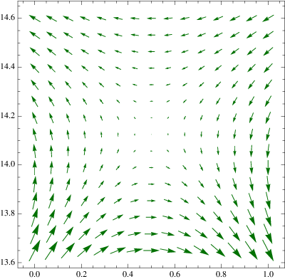
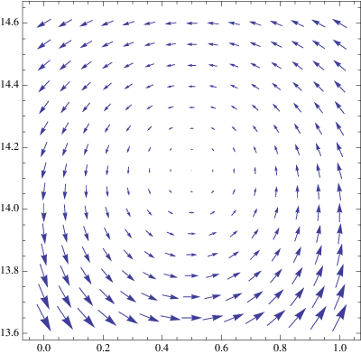
We now turn to the global properties of along the entire critical strip. It is not difficult to see that the vorticity of the Riemann zeros on the critical line, or , alternate in sign as one moves along it. Otherwise, the curl of would not be zero in a region between two consecutive zeros. Thus there is a form of quasi-periodicity along the critical line, in the sense that zeros alternate between being even and odd, like the integers, and also analogous to the zeros of at where . A proof of this alternating vorticity requires some analysis of the function , which is described in section IV. Also, along the nearly horizontal contours that cross the critical line, is in the direction. This leads to the pattern in Figure 5. One aspect of the rendition of this pattern is that it implicitly assumes that the and points along the line alternate, namely, between two consecutive points along this line, there is only one point, which is consistent with the knowledge that there are no zeros of along the line . This fact will be clearer when we reformulate our argument in terms of the potential below.

Let us now consider the possibility of a Riemann zero elsewhere on the critical strip, i.e. off of the critical line. The only location this could occur is along a contour that intersects the critical line. In order for a Riemann zero to exist there requires a contour to intersect the contour, and recall they must be perpendicular at the intersection. Such a contour, of the kind that does not cross the critical line, is shown in Figure 1. In comparison with the zeros on the critical line, the and contours are nearly rotated by . This leads to a “frustration” of the electric field. Namely, as Figure 5 indicates, wants to be horizontal at such a location, but if there exists a contour here, this would imply the electric field would be vertical along it, as shown in Figure 6. Since the pattern in Figure 5 very likely repeats itself all along the critical strip because of the known infinity of zeros along it, this frustration appears to be inconsistent, and this suggests that such a Riemann zero would appear to be impossible, although this is not yet a proof. One needs to establish that the pattern in Figure 5 indeed regularly repeats itself all along the critical strip.
The RH is equivalent to the statement that all contours cross the critical line and span the entire strip. We have argued that this follows from the existence of the infinite number of zeros along the critical line, the identity eq. (7), and the global properties of the field which are a consequence of the existence of these zeros. To strengthen this picture, one needs to more accurately define the notion of “frustration” in this context. In the next section, a more concrete analysis will be based on the potential . A related remark is that the properties of depicted in Figure 5 require that the and points along the line are well separated, and this is consistent with the proven fact that there are no roots to the equation , which can be used to prove the Prime Number Theorem[1].

III The electric potential
A mathematically integrated version of the above arguments, which has the advantage of making manifest the dependency of and , can be formulated in terms of the electric potential which is a single real function. Although it contains the same information as the above argument, it is more economical, and more importantly, because it does not rely on properly defining the notion of “frustration” in order to make the argument. By virtue of , is also a solution of Laplace’s equation where . The general solution is that is the sum of a function of and another function of . Since must be real,
| (12) |
where . Clearly is not analytic, whereas is; it is useful to work with since we only have to deal with one real function. Comparing the definitions of and in terms of , one finds and . The latter implies
| (13) |
This equation can be integrated because is entire. Using an integral representation for derived in Riemann’s original paper, one can show that up to an irrelevant additive constant,
| (14) |
where is the -derivative of the function , and is one of the four elliptic theta functions.
Let us now consider the contours in the critical strip. Using the integral representation eq. (14), one finds the symmetry . One sees then that the contours do not cross the critical line, whereas the contours can and do. Since is imaginary along the critical line, the latter is also a contour. Thus the contours have the same structure as those for shown in Figure 1.
All Riemann zeros necessarily occur at isolated points, which is a property of entire functions. This is clear from the factorization formula , conjectured by Riemann, and later proved by Hadamard. Where are these zeros located in terms of ? At , . Thus, such isolated zeros occur when two contours intersect, which can only occur if the two contours correspond to the same value of since is single-valued. A useful analogy is the electric potential for equal point charges. The electric field vanishes halfway between them, and this is the unique point where the equi-potential contours vanish. The argument is simple: is perpendicular to the contours, however as one approaches along one contour, one sees that it is not in the same direction as inferred from the approach from the other contour. The only way this could be consistent is if at .
With these properties of , we can now begin to understand the location of the known Riemann zeros. Since the contours intersect the critical line, which is also a contour, a zero exists at each such intersection, and we know there are an infinite number of them. The contour plot in Figure 7 for the actual function constructed above verify these statements. We emphasize that there is nothing special about the value , since can be shifted by an arbitrary constant without changing ; we defined it such that the critical line corresponds to .

A hypothetical Riemann zero off of the critical line would then necessarily correspond to an intersection of two contours. For simplicity, let us assume that only two such contours intersect, since our arguments can be easily extended to more of such intersections. Such a situation is depicted in Figure 8. This figure implies that on the line , specifically , takes on the same non-zero value at four different values of between consecutive zeros, i.e. roots of the equation , where . Thus, the real function would have to have 3 extrema between two consecutive zeros. Figure 7 suggests that this does not occur. In order to begin to prove it, let us define a “regular alternating” real function of a real variable as a function that alternates between positive and negative values in the most regular manner possible: between two consecutive zeros has only one maximum, or minimum. For example, the function is obviously regular alternating. By the above argument, if is regular alternating, then two contours cannot intersect and there are no Riemann zeros off the critical line.

To summarize this section, based on the symmetry eq. (7), and the existence of the known infinity of Riemann zeros along the critical line, we have argued that and satisfy a regular repeating pattern all along the critical strip, and the RH would follow from such a repeating pattern. In order to go further, one needs to investigate the detailed properties of the function , in particular it’s large asymptotic behavior, and establish its repetitive behavior, more specifically, that it is a regular alternating function. This is the subject of the next section, which is more constructive.
IV Analysis and an asymptotic formula for the -th Riemann zero.
As in the Introduction, define , which also has the symmetry . It has a pole at , but this does not affect the analysis of the zeros for large on the critical strip. Let us represent as . Define as with the Stirling formula approximation to . This approximation breaks the symmetry, but since we know it exists, we can easily restore it:
| (15) |
One can show that for large ,
| (16) | |||||
Let us now show for , this approximation for large has no zeros, since its real and imaginary parts, which just involve sine’s and cosine’s of the -function of the exponential in eq. (16), cannot simultaneously be zero. To be more specific, requiring that both the real and imaginary parts of this approximation to be zero leads to the two equations
| (17) |
where is the argument of the exponential in eq. (16), , and where is the overall real factor multiplying the exponential in the above equation. In order to be more rigorous, one should shift away from a zero with a small complex number , i.e. consider . In this way, when is not strictly zero, one can first safely divide by in order to obtain eq. (17), and then take the limit . Squaring these two equations, one finds that they imply . However since for any , there are no solutions, except for . Although as one approaches a zero, both and are zero because of the factor, their ratio is well defined and indeed equals , so the above argument is consistent.
The solution of the above equations (17), with , that corresponds to the zeros is
| (18) |
This is not the most general solution to (17), but the other solutions are inconsistent with the functional relation. The constraint implies . Thus for large , there are no Riemann zeros off of the critical line.
The above analysis leads to an explicit equation satisfied by the -th zero which depends only on . The equation (18) shows that the Riemann zeros are in one-to-one correspondence with the zeros of the cosine, i.e. occur when , where is an integer. In order to conform with the standard definition of the -th zero by comparing with the lowest zeros, one must chose , and one finds that the -th Riemann zero is of the form , , where satisfies the following equation:
| (19) |
where we have dropped the terms.
It follows that eq. (19) implies that the number of zeros along the critical line with is given by the above expression with and :
| (20) |
The result above was obtained by Riemann for the zeros on the entire critical strip[3]. The correction is due to Backlund[1]. Riemann knew about the additional . The latter has also been obtained from quantization of the Berry-Keating hamiltonian[5, 19, 20]. However, eq. (19) is a stronger result since it is for zeros on the critical line and is an equation satisfied by each individual zero which depends only on . It should be stressed that although the two equations (19) and (20) resemble each other, it is impossible to derive the former from the latter, again because the latter has only been proven for the entire strip assuming is not the ordinate of a zero. It is clearly stated in Edward’s book that has never been shown to be valid on the critical line.
The is small compared to the other terms. This leads to a simple approximation of the -th zero on the critical line, Dropping this term, is a solution of the transcendental equation
| (21) |
The solution is explicitly given in terms of Lambert’s W-function[18]
| (22) |
Although this just a simple inversion, it is quite useful since the Lambert function is implemented in most numerical packages. The above formula neither misses zeros nor predicts non-existent zeros, i.e. every zero is in the vicinity of for some , and there are no zeros between and .
The above formula is closely related, but not identical, to the Gram points , which are solutions to where is the Riemann-Siegel function. We have not used the function in the analysis of this paper. The Gram point that is closest to the first zero is , compared to our which is much closer to the true zero. Gram’s Law is the tendency for Riemann zeros to lie between consecutive Gram points, but it is known to fail for about of all Gram intervals[1]. Our result is essentially different, in that the eq. (21) is an asymptotic formula for the actual zeros and is thus somewhat stronger than Gram’s criterion, which in any case is known to be violated.
Table 1 shows how well the formula (22) works for various up to , where for the latter the fractional error is about . This confirms the validity of the approximations we have made. Tables of zeros were calculated to high accuracy by Odlyzko, which in part relies on the Gram points, and can be found at his website [21]. The two adjacent zeros at 1 million indicates that eq. (21) can accurately distinguish nearby zeros. Here is our estimate of the -th zero:
| (23) |
and is exact to the number of digits shown, and actually much more: the Lambert function approximation is here accurate to a million digits, which we were easily able to calculate with Mathematica. The approximation (22) for the ’th zero is correct to roughly digits.
| n | exact | solution to eq. (21) |
|---|---|---|
| 10 | 49.8 | 50.2 |
| 100 | 236.5 | 236.0 |
| 1000 | 1419.4 | 1419.5 |
| 10,000 | 9877.8 | 9877.6 |
| 100,000 | 74920.8 | 74920.9 |
| 1,000,000 | 600269.7 | 600269.6 |
| 1,000,001 | 600270.3 | 600270.2 |
| 10,000,000 | 4992381.0 | 4992381.1 |
| 267653395648.8 | 267653395649.0 | |
| 1370919909931995308226.68 | 1370919909931995308226.77 |
The term in eq. (20) oscillates around zero, and changes sign in the vicinity of each Riemann zero. It is thus responsible for turning the smooth part of into a staircase function that actually counts the zeros[4, 5]. At a zero it can be defined by the well-defined limit . The latter is generally not zero. For instance, for the first Riemann zero, . Equation (19) indeed improves the estimates of the Riemann zeros of the last section. It is more difficult to solve numerically, but simple root-finder software such as in Mathematica can easily solve the equation by searching for a solution in the vicinity of the approximation in eq. (22). The result is surprisingly accurate. For the first zero it gives
| (24) |
which is correct to the number of digits shown[21]. This strongly suggests that the corrections in eq. (19) are completely under control.
Montgomery’s pair correlation conjecture[22] relates the statistics of the zeros to that of random Hermitian matrices in the GUE universality class[23]. Strong evidence for this conjecture was given by Odlyzko[24]. It is known that the fluctuating correction in eq. (19) is important for such statistics[4, 5].
Let us return to the statement that the validity of the RH is equivalent to the property that of the last section is a regular alternating function. Away from the pole at , as in section II we can define an electric field from the real and imaginary parts of , which also has zero divergence and curl, and . The same arguments as in section II apply, and the RH follows if is a regular alternating function. For large , this follows from the log-periodic behaviour in eq. (16), i.e. .
The formulas of this section can also be used to demonstrate the statement made in section II that the vorticity of the zeros alternate in sign as one moves up the critical line. The latter implies that the electric field, which is horizontal along the critical line, changes direction at a zero, but between zeros is always either to the left or right, as depicted in Figure 5. This follows again from the periodic behavior of along the critical line, i.e. .
V Concluding Remarks
In summary, our analogy with the electric field and potential suggested a very regular pattern of the function in the critical strip. We argued that the RH follows if the real function on the line , or equivalently , is what we referred to as a regular alternating function of . This motivated the analysis of the last section, which revealed such a pattern, more specifically the log-periodic behavior we derived in eq. (16). This led to the simple formulas (21) and (19) for the n-th Riemann zero at large . The approximations in section IV that led to eq. (19) are well controlled, as indicated by the fact that accurate values for even the lowest zeros can be obtained from it.
The equations (19) and (21) are equations that determine the zeros on the critical line, and Riemann’s counting formula eq. (2) for the zeros on the entire strip is a consequence of them, including the corrections in eq. (20). We also provided additional analysis in the last section showing that there are no zeros off of the critical line with sufficiently large imaginary part. Our work thus indicates an extreme regularity of the zeros with large imaginary part. Since it is already known that there are no zeros off the line for or more[21, 3], this would seem to establish the RH, especially since the equation (19) is nearly identically satisfied even for the lowest zeros.
Note added: We have recently published two follow-up’s to this article[25] wherein we show that the solutions of eq. (19) are accurate enough to reveal the GUE statistics. We also provide a more rigorous treatment of section IV, and derive an exact version of eq. (19), which completely controls the corrections. We have also generalized the equations of the last section to arbitrary Dirichlet L-functions[26].
VI Acknowledgments
I especially wish to thank Giuseppe Mussardo for useful discussions and the hospitality of the ICTP and SISSA in Trieste, Italy, where this work was nearly completed. Germán Sierra and Andrew Odlyzko provided useful comments on the manuscript, in particular the similarity of our with Gram points which I was previously unaware of. In particular, Sierra suggested to try and obtain the fluctuating part in which we presented in section IV. I also wish to thank Guilherme França for subsequent discussions on the GUE statistics of the Riemann zeros.
I also wish to thank Olus Boratav, for challenging me a few years ago to write a popular article on the Riemann Hypothesis, and this only recently re-awakened my interest. In any case, there is already an excellent popular book on the subject[27]. This work is supported by the National Science Foundation of the United States of America under grant number NSF-PHY-0757868.
References
- [1] H. M. Edwards, Riemann’s Zeta Function, Dover Publications Inc. 1974.
- [2] In the mathematics literature the complex variable is conventionally denoted as in this context. Here the notation will be since this makes the vectorial aspects we will consider more natural.
- [3] J. B. Conrey, The Riemann Hypothesis, Notices of the AMS 50 (2003) 342.
- [4] M. V. Berry, Riemann’s Zeta Function: A Model for Quantum Chaos?, Quantum Chaos and Statistical Nuclear Physics, Eds. T. H. Seligman and H. Nishioka, Lecture Notes in Physics, 263 Springer Verlag, New York, 1986.
- [5] M. V. Berry and J. P. Keating, The Riemann zeros and eigenvalue asymptotics, SIAM Review 41 (1999) 236.
- [6] M. V. Berry and J. P. Keating, H=xp and the Riemann zeros, in Supersymmetry and Trace Formulae: Chaos and Disorder, Kluwer 1999.
- [7] G. Sierra, The Riemann zeros and the cyclic Renormalization Group, J. Stat. Mech. 0512:P12006, 2005.
- [8] G. Sierra, A Quantum Mechanical model of the Riemann Zeros, NewJ. Phys. 10 (2008) 033016.
- [9] D. Schumayer and D. A. W. Hutchinson, Physics of the Riemann Hypothesis, Rev. Mod. Phys. 83 (2011) 307 [arXiv:1101.3116].
- [10] G. Sierra and P. K. Townsend, Landau levels and Riemann zeros, Phys. Rev. Lett. 101 (2008) 110201.
- [11] G. Sierra and J. Rodriguez-Laguna, The H=xp model revisited and the Riemann zeros, Phys. Rev. Lett. 106 (2011) 200201.
- [12] A. Connes, Trace formula in non-commutative geometry and the zeros of the Riemann zeta function, Sel. Math. New Ser. 5 (1999) 29.
- [13] A translated version of his paper can be found in [1].
- [14] A. LeClair, Interacting Bose and Fermi gases in low dimensions and the Riemann Hypothesis, Int. J. Mod. Phys. A23 (2008) 1371 [arXiv:math-ph/0611043].
- [15] S. Coleman, There are no Goldstone bosons in two dimensions, Commun. Math. Phys. 31, 259 (1973).
- [16] N. D. Mermin and H. Wagner, Absence of ferromagnetism or antiferromagnetism in one- or two- dimensional isotorpic Heisenberg models, Phys. Rev. Lett. 17, 1133 (1966).
- [17] See for instance the website: functions.wolfram.com.
- [18] I thank Guilherme França for pointing this out.
- [19] G. Sierra, The Riemann zeros and the cyclic Renormalization Group, J. Stat. Mech. 0512:P12006, 2005.
- [20] R. K. Baduri, A. Khare and J. Law, The Phase of the Riemann Zeta Function and the Inverted Harmonic Oscillator, Phys. Rev. E52 (1995) 486.
- [21] A. Odlyzko, Tables of zeros of the Riemann zeta function, www.dtc.umn.edu/ odlyzko/zeta-tables/.
- [22] H. Montgomery, The pair correlation of zeros of the zeta function, Analytic number theory, Proc. Sympos. Pure Math. XXIV, Providence, R.I.: American Mathematical Society, pp. 181Ð193, 1973.
- [23] F. Dyson, Correlations between eigenvalues of a random matrix, Comm. Math. Phys. 19 (1970) 235.
- [24] A. M. Odlyzko, On the Distribution of Spacings Between Zeros of the Zeta Function, Mathematics of Computation 177 (1987) 273.
- [25] G. França and A. LeClair, Statistical and other properties of Riemann zeros based on an explicit equation for the -th zero on the critical line, arXiv:1307.8395.
- [26] G. França and A. LeClair, On the zeros of Dirichlet L-functions, arXiv:??????.
- [27] J. Derbyshire, PRIME OBSESSION. Bernhard Riemann and the Greatest Unsolved Problem in Mathematics, Joseph Henry Press, Washington, D.C. 2008.