Quantum simulations of localization effects with dipolar interactions

The initial state $\rho_{0}$ of the uncorrelated spins commutes with $\widehat{\mathcal{H}}_{dd}$. Therefore, to generate spin clusters we use an NMR method developed by Pines and coworkers [61, 62]. It is based on generating an average Hamiltonian $\widehat{\mathcal{H}}_{0}$ that does not commute with the thermal equilibrium state

This Hamiltonian drives an evolution that converts the thermal initial state into clusters of correlated spins whose density operator contains terms of the form $\hat{I}_{u}^{i}...\hat{I}_{v}^{j}\hat{I}_{w}^{k}\left(u,v,w=x,y,z\right)$, where the indexes $i,j,k$ identify the spins involved in the given cluster. The cluster-size $K$ corresponds to the number of terms in this product, which is equal to the number of spins. The cluster size is related to the volume occupied by those spins. Experimentally, the Hamiltonian $\widehat{\mathcal{H}}_{0}$ is generated with the pulse sequence [61, 62] shown in the upper part of Fig. 2.

In the usual computational or Zeeman basis $\left|\alpha_{1},\alpha_{2},...,\alpha_{K}\right\rangle$ ($\alpha_{i}=\uparrow,\downarrow$) for a system of $K$ spins, we write the states as $\left|M_{z},n_{M}\right\rangle$ where $M_{z}$ is the total magnetic quantum number, i.e., $\hat{I}_{z}\left|M_{z},n_{M}\right\rangle=M_{z}\left|M_{z},n_{M}\right\rangle$, and $n_{M}$ distinguishes different states with the same $M_{z}$. Figure 3a shows a summary of these states, whose degeneracy is $\max\left\{n_{M}\right\}=K!/\left[\left(K/2-M_{z}\right)!\left(K/2+M_{z}\right)!\right]$.

The Hamiltonian $\widehat{\mathcal{H}}_{0}$ flips simultaneously two spins, which are separated in space and have the same orientation. Accordingly, the $z$-component of the magnetization $M_{z}$ changes by $\Delta M_{z}=\pm 2.$ This is shown with a curved solid arrow in Fig. 3a. At the same time, the number $K$ of correlated spins changes by $\Delta K=\pm 1$. Therefore, starting from the thermal equilibrium state, the evolution generates a density operator where only elements $\rho_{ij}$ with $\Delta M=M_{z}(i)-M_{z}(j)=2n,\,n=0,1,2\dots$ are populated. Such elements $\rho_{ij}$ are called $\Delta M$ quantum coherences and they are represented by colored straight arrows in Fig. 3a. The different colors represent different multiple-quantum coherence (MQC) orders $\Delta M$. Off-diagonal elements of the density matrix with $\Delta M=0$ represent zero-quantum coherences and diagonal elements correspond to populations. Then, a MQC spectrum $A(\Delta M)$ can be described by the number of coherences of the density matrix for a given $\Delta M$. A typical MQC spectrum is shown in Fig. 3b. The initial state $\rho_{0}$ is diagonal and then $A(\Delta M)\neq 0$ only for $\Delta M=0$. However, as time evolves, different spins interact with each other and other coherence orders are excited. Then $A(\Delta M)$ starts to spread as a manifestation of the increasing cluster-size. If we measure the evolution of the operator $I_{z}$ as a function of time, $\left\langle I_{z}(t)\right\rangle=\mathrm{Tr}\left\{I_{z}\rho(t)\right\}$, its expectation value decays as a consequence of the excitation of the coherences of the density matrix that do not contribute to the observable $\left\langle I_{z}(t)\right\rangle$. The black squares in Fig. 4 show the evolution of $\left\langle I_{z}(t)\right\rangle$ driven by the Hamiltonian $\widehat{\mathcal{H}}_{0}$.

We can see a fast decay on a time scale of $\approx 100\,\mu$s, which is followed by a quantum beat at about 400$\mu$s. Then the signal saturates.

To determine the average number of correlated spins in the generated clusters, we use the NMR technique developed by Baum et al. [62]. In a system of $K$ spins, the number of transitions with a given $\Delta M$ follows a binomial distribution

For $K\gg 1,$ the binomial distribution can be approximated with a Gaussian

whose half width at $e^{-1}$ is $\sigma=\sqrt{K}$ . Thus, the width of the MQC spectrum reflects the cluster-size. We can determine the effective size of the spin clusters in a given state by measuring the distribution of the MQCs of its density operator $\rho$ as a function of the coherence order $\Delta M$. They can be distinguished experimentally by rotating the system around the $z-$axis: a rotation $\hat{\phi}_{z}=e^{-i\phi\hat{I}_{z}}$ by $\phi$ changes the density operator to

where $\hat{\rho}_{\Delta M}$ contains all the elements of the density operator involving coherences of order $\Delta M$.

By following the sequence of Fig. 2, the system evolution is first described by an evolution period of duration $N\tau_{0}$ under the Hamiltonian $\left(\mathcal{\widehat{H}}_{0}\right)_{\phi}=\hat{\phi}_{z}\mathcal{\widehat{H}}_{0}\hat{\phi}_{z}^{\dagger}$, i.e.,

The next part of the sequence of Fig. 2 is an evolution of the same duration $N\tau_{0}$ under $-\mathcal{\widehat{H}}_{0}$. This causes an evolution backward in time that gives the following density operator at the end of the sequence

If $\hat{I}_{z}$ is the NMR observable, then the signal becomes

where $A(\Delta M)$ are the amplitudes of the MQ spectrum shown in Fig. 3b. To extract these amplitudes from the experimental data, we measure the signal $\left\langle\hat{I}_{z}\right\rangle\left(\phi,N\tau_{0}\right)$ as a function of $\phi$ at a fixed time $N\tau_{0}$ and then perform a Fourier transform with respect to $\phi$ as shown schematically in Fig. 5 (Black squares). The cluster size is then determined by the half-width at $e^{-1}$, $\sigma=\sqrt{K}$, of $A(\Delta M)$.

Figure 6 shows the time evolution of the measured cluster size $K\left(N\tau_{0}\right)$ as a function of the total evolution time $N\tau_{0}$. For the unperturbed Hamiltonian, the cluster size appears to grow indefinitely [35, 36]. The figure also shows two examples of the $A(\Delta M)$ distributions at different times. We can see that for long times $K\propto\left(N\tau_{0}\right)^{4.3}$. Assuming that the cluster-size $K$ is associated with the number of spins inside a volume, it is seen that the associated length grow faster than normal diffusion, where its growing curve would be expected to be $\propto\left(N\tau_{0}\right)^{3/2}$.

This evolution can be reversed completely by changing the Hamiltonian from $\widehat{\mathcal{H}}_{0}$ to $-\widehat{\mathcal{H}}_{0}$. Experimentally, this is achieved by shifting the phase of all RF pulses by $\pm\pi/2$ [61]. The signal $\left\langle I_{z}\right\rangle\left(\phi,N\tau_{0}\right)$ at the end of the sequence of Fig. 2 is a time reversal echo for $\phi=0$. This means that under ideal conditions $\sum_{M}A(\Delta M,N\tau_{0})=\mathrm{const}$ and we will write $E\left(N\tau_{0}\right)$ for this quantity. The indefinite growth of the cluster size, as well as the complete reversibility of the time evolution are no longer possible if the effective Hamiltonian deviates from the ideal form (7).

Experimentally, the Hamiltonian $\widehat{\mathcal{H}}_{0}$ is generated as an effective Hamiltonian by the pulse sequence of Fig. 2. Because of experimental imperfections, it always deviates from the ideal Hamiltonian (7). As a result, the actual dynamics deviates from the ideal one and, in particular, we cannot invert exactly the perturbed Hamiltonian and thus reverse the time evolution perfectly. The quantity $\sum_{\Delta M}A(\Delta M)$ is no longer conserved, but decays with increasing evolution time.

The ideal form of the effective Hamiltonian (7) can only be created if the dipolar couplings $d_{i,j}$ are time independent and the pulses are ideal and rotate globally all the spins. However, if these couplings are time dependent, or the pulses are not ideal, the effective Hamiltonian (averaged over the pulse cycle) contains additional terms. We have partly characterized the spectral density of local spin-spin fluctuations driven by $\widehat{\mathcal{H}}_{dd}$ in Ref. [63, 55] and its correlation time was about $\tau_{d}=110\mu$s. Since the imperfection on $\widehat{\mathcal{H}}_{0}$ are correlated with the fluctuations driven by $\widehat{\mathcal{H}}_{dd}$, we can use $\tau_{d}$ to estimate the correlation time of the fluctuations of the $\widehat{\mathcal{H}}_{0}$ imperfections.

In Fig. 6 the cluster size grows faster for times lower than $\tau_{d}$. After $\tau_{d}$ the cluster size growth reduces speed and seems to start growing exponentially [35, 36]. After 1ms, the growing law again change its behavior and the cluster size grows as a power law [35, 36]. We cannot contrast this regime with the spectral density determined in Ref. [63] because it was not determined for the corresponding range of frequency fluctuations. While all these regimes cannot be rigorously determined, there is a fact that the cluster-size keeps growing for long time and faster than normal diffusion. This ‘super-diffusion’ may be a result of the long range nature of the dipolar interaction [64, 65].

In previous works [35, 36] and in Fig. 6, we determined the cluster growth by isolating the intrinsic decay generated by an imperfect effective Hamiltonian (7). The imperfection effects are manifested in the overall decrease of the echo signal $E\left(N\tau_{0}\right)$ by normalizing the MQ spectra such that the total signal $\sum_{\Delta M}A(\Delta M)$ for $\phi=0$ is constant in time. Now, we measured the decay of $E\left(N\tau_{0}\right)=\sum_{\Delta M}A(\Delta M,N\tau_{0})$. The results are shown in Fig. 7. If we consider the imperfections on $\widehat{\mathcal{H}}_{0}$, the effective Hamiltonian during the first part of the sequence of Fig. 2a will be $\widehat{\mathcal{H}}_{fwd}=\widehat{\mathcal{H}}_{0}+\widehat{\mathcal{H}}_{e}$, and $\widehat{\mathcal{H}}_{bwd}=-\widehat{\mathcal{H}}_{0}+\widehat{\mathcal{H}}_{e}^{\prime}$ during the time reversed part, where $\widehat{\mathcal{H}}_{e}$ is an average error Hamiltonian. The echo decay is then $E(N_{0}\tau_{0})=\mathrm{Tr}\left\{\hat{\rho}^{\mathcal{H}_{fwd}}\left(N\tau_{0}\right)\hat{\rho}^{\mathcal{H}_{bwd}}\left(N\tau_{0}\right)\right\}$ and it quantifies the time reversal probability as a kind of Loschmidt echo [24, 25, 66].

The echo decay $E(N_{0}\tau_{0})$ shown in Fig. 7 starts as a Gaussian for times shorter than $N_{0}\tau_{0}\lesssim 288\mu$s$\approx 2.6\,\tau_{d}$. For longer times it decays exponentially until $\approx 920\mu$s where a different decay law arises. These transitions between different decay laws seems to be correlated with the growing law transitions discussed in the previous parragraphs. This resembles the typical behavior of nuclear spins of a solution diffusing in a inhomogeneous magnetic field with a given standard deviation [67] or in restricted spaces in the presence of a magnetic field gradient [68]. If the spins only interact with the magnetic field, due to the diffusion process, they feel a different magnetic field at different times causing dephasing of the spin signal. The frequency fluctuations have a correlation time given by the time needed to explore the standard deviation of the changes of the magnetic field that is related with the inhomogenity of the magnetic field or to the restriction length. By applying a spin-echo sequence -a time reversion of the spin precession by an inversion pulse that changes the sign of the magnetic field interaction- one can partly reverse the effects of the diffusion-driven dephasing [69, 70]. The echo sequence is analogous to the one of Fig. 2. If the inversion pulse inducing the time reversal is applied at times shorter than the correlation time of the frequency fluctuations of the spins, the signal decay depends of the spatial displacement of the spins and the signal decays faster as the time passes because the dephasing rate increases with the displacement length. However, for times longer than the correlation time of the frequency fluctuations the decay rate becomes independent of the displacement and becomes exponential, similar to the time reversal echo behavior shown in Fig. 7.

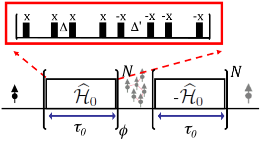
The echo decay in Fig. 7 depends of perturbation $\widehat{\mathcal{H}}_{e}$. In order to study the sensitivity to the perturbation strength, we introduced a perturbation $\widehat{\Sigma}$, whose strength we can control experimentally and study the behavior of the system as a function of the perturbation strength. We choose the raw dipole-dipole coupling for this perturbation, $\widehat{\Sigma}=\mathcal{\widehat{H}}_{dd}$, which has long range interactions with coupling strengths decaying as $1/r^{3}$. We add this Hamiltonian to the ideal Hamiltonian $\widehat{\mathcal{H}}_{0}$ by concatenating short evolution periods under $\widehat{\mathcal{H}}_{dd}$ with evolution periods under $\widehat{\mathcal{H}}_{0}$. We label the durations of the two time periods $\tau_{\Sigma}$ and $\tau_{0}$, as shown in Fig. 8.

When the duration $\tau_{\mathrm{c}}=\tau_{0}+\tau_{\Sigma}$ of each cycle is short compared to the inverse of the dipolar couplings $d_{ij}$, the resulting evolution can be described by the effective Hamiltonian

where the relative strength $p=\tau_{\Sigma}/\tau_{\mathrm{c}}$ of the perturbation $\widehat{\Sigma}=\widehat{\mathcal{H}}_{dd}$ can be controlled by adjusting the duration $\tau_{\Sigma}$. For the quantum simulations, we compared the artificially perturbed evolution of $\widehat{\mathcal{H}}_{\mathrm{eff}}$ with the $\widehat{\mathcal{H}}_{0}$ evolution with its intrinsic errors. While the intrinsic errors reduce the signal or the overall fidelity, they do not cause localization on the time scale of our experiments (see Fig. 6).

Starting from thermal equilibrium, now the state of the system at the end of $N$ cycles is $\hat{\rho}^{\mathcal{H}_{\mathrm{eff}}}\left(N\tau_{\mathrm{c}}\right)=e^{-i\widehat{\mathcal{H}}_{\mathrm{eff}}N\tau_{\mathrm{c}}}\hat{\rho}_{0}e^{i\widehat{\mathcal{H}}_{\mathrm{eff}}N\tau_{\mathrm{c}}}.$ Taking into account now the complete sequence of evolutions given by Fig. 2b, the experiment is thus a perturbed forward evolution and an unperturbed backward evolution. The density matrix at the end of the sequence is then $\sum_{M}\left[e^{i\mathcal{\widehat{H}}_{0}N\tau_{0}}\hat{\rho}_{M}^{\mathcal{H}_{\mathrm{eff}}}\left(N\tau_{\mathrm{c}}\right)e^{-i\mathcal{\widehat{H}}_{0}N\tau_{0}}\right]e^{iM\phi}$ as derived in [35, 36]. Thus the NMR echo signal, which is measured after the last backward evolution $\exp\left\{i\widehat{\mathcal{H}}_{0}N\tau_{0}\right\}$, can be written as

In terms of the individual MQ coherences, this may be written as

with the MQ coherence amplitudes $A(\Delta M)=\mbox{Tr}\left\{\hat{\rho}_{\Delta M}^{\mathcal{H}_{0}}\left(N\tau_{0}\right)\hat{\rho}_{\Delta M}^{\mathcal{H}_{\mathrm{eff}}}\left(N\tau_{\mathrm{c}}\right)\right\}$. For the ideal evolution ($p=0$), Eq. (14) is recovered, where $A(\Delta M)$ correspond to the squared amplitudes of the density operator elements $\hat{\rho}_{\Delta M}^{\mathcal{H}_{0}}\left(N\tau_{0}\right)$ with coherence order $\Delta M$. For the perturbed evolution, $(p\neq 0)$, they are reduced by the overlap of the actual density operator elements $\hat{\rho}_{\Delta M}^{\mathcal{H}_{\mathrm{eff}}}\left(N\tau_{\mathrm{c}}\right)$ with the ideal ones. We extract these amplitudes by performing a Fourier transformation with respect to $\phi$. Figure 9 shows a comparison between the distributions $A(\Delta M)$ for different evolution times for an unperturbed evolution (panel a) and a perturbed evolution with $p=0.108$ (panel b). The main difference is that the MQC spectrum of the perturbed evolution does not spread indefinitely but its width reaches a limiting value [35, 36].

As discussed in section III.1.2, we determine the cluster size for different evolution times and perturbation strengths from the width of the measured MQC distributions. Figure 10 shows the cluster size (the number of correlated spins) as a function of the evolution time $N\tau_{c}$. The main difference of the perturbed time evolutions (colored symbols in Fig. 10) compared to the unperturbed evolution (black squares) is that the cluster size does not grow indefinitely [35, 36], but saturates. It remains unclear if the cluster growth for the weakest perturbation $p=0.009$ also saturates. We consider this saturation as evidence of localization due to the perturbation and the localization size decreases with increasing the perturbation strength $p$. .