Numerical Reparametrization of Rational Parametric
Plane Curves
Sonia Pérez-Díaz
Email: sonia.perez@uah.esAddress: Dpto. de Física y Matemáticas,
Universidad de Alcalá,
E-28871 Madrid, Spain
Li-Yong Shen
Email: shenly@amss.ac.cnAddress: School of Mathematical Sciences, University of
CAS, Beijing, China
Corresponding author: Corresponding author
Abstract
In this paper, we present an algorithm for reparametrizing
algebraic plane curves from a numerical point of view. That is, we deal with mathematical objects that are assumed to be given approximately. More precisely, given a tolerance and a rational parametrization with perturbed float coefficients of a plane curve , we present an
algorithm that computes a parametrization of a new plane curve such that is an –proper reparametrization of . In addition, the error bound is carefully discussed and we present a formula that measures the “closeness" between the input curve and the output curve
.
A rational parametrization of an algebraic plane curve
establishes a rational correspondence of
with the affine or projective line. This correspondence is a birational
equivalence if is proper i.e., if traces the curve once. Otherwise, if is not proper, to almost all points on , there corresponds more than one parameter value. Lüroth’s theorem shows constructively that it is always possible to reparametrize an improperly parametrized curve such that it becomes properly parametrized. That is, to almost all points (except perhaps finitely many) there corresponds exactly one parameter value such that . A proper reparametrization always reduces the degree of the rational functions defining the curve.
The reparametrization problem, in particular when the variety is a curve or a
surface, is specially interesting in some practical applications
in computer aided
geometric design (C.A.G.D) where objects are often given and manipulated
parametrically. In addition, proper parametrizations play an
important role in many practical applications in C.A.G.D, such as in visualization (see [13],
[14]) or rational parametrization of offsets (see
[2]). Also, they provide an implicitization approach based
on resultants (see [9] and [25]). Hence, the study of proper reparametrization has been concerned by some authors such as [5, 17, 18, 25, 27], and several efficient proper reparametrization
algorithms can be found
in [12, 17, 24].
The problem of proper reparametrization for curves has been widely discussed in symbolic consideration. More precisely, given the field of complex numbers , and a rational
parametrization of an algebraic
plane curve with exact
coefficients, one finds a rational proper parametrization
of , and a rational
function such that . Nevertheless, in many practical applications, for instance in the frame of
C.A.G.D, these approaches tend to be insufficient, since in
practice most of data objects are given or become approximate. As a consequence, there has been an increasing interest for the development of hybrid
symbolic-numerical algorithms, and approximate algorithms.
Intuitively speaking,
one is given a tolerance
, and an irreducible affine algebraic plane curve
defined by a parametrization with perturbed float coefficients that is “nearly improper" (i.e. improper within the tolerance ), and the problem consists in computing a rational
curve defined by a parametrization , such that is proper and almost all points of the rational curve are in the “vicinity" of . The notion of vicinity may be introduced
as the offset region limited by the external and internal offset
to at distance (see Section 4 for more
details), and
therefore the problem consists in finding, if it is possible, a
rational curve properly parametrized and lying within the offset
region of . For instance, let us suppose that we are
given a tolerance , and a curve defined by the parametrization
Figure 1: Input curve (left), curve (center), curves and (right)
One may check that is proper in exact consideration
but it is nearly improper since for almost all points , there exist two values of the parameter , given by the approximate roots of the equation
such that is “almost equal" to . Our method provides as
an answer the curve defined by the -proper reparametrization
In Figure 1, one may check that and are “close".
The problem of relating the tolerance with the vicinity notion, may be approached either analyzing locally the condition number of the implicit equations (see [10]) or studying whether for almost every point on the original curve, there exists a point on the output curve such that the euclidean distance of and is significantly smaller than the tolerance. In this paper our error analysis will be based on the second approach. From this fact, and using [10], one may derive upper bounds for the distance of the offset region.
Approximate algorithms have been developed for some applied numerical topics, such as, approximate parametrization of algebraic curves and surfaces [19, 20, 23], approximate greatest common divisor (gcd) [3, 4, 7, 15, 16, 32], finding zeros of multivariate systems [7], and factoring polynomials [6, 11]. Few papers discussed the problem of properly
reparametrizing a given parametric curve with perturbed float coefficients.
As we know, only a heuristic algorithm was proposed in [24]. However, the error analysis is not discussed, and no step is given to detect whether
a numerical curve is improper within a tolerance. In symbolic considerations, the tracing index is used to determine the properness of a parametrization of an algebraic plane curve (see [25, 30]). Essentially, it is the cardinality of a generic fibre of the parametrization, and from the geometric point of view, the tracing index measures the number of times that a parametrization
traces a curve over the algebraic closure of the ground field. In this paper, we extend the concept to
the numerical situations that is, the approximate improper index is expected to be the number
of parameter value mapped in a neighborhood to a generic point of a given plane curve.
This gives the theoretical foundation for our further discussion.
In this paper, we review the symbolic algorithm of reparametrization for algebraic plane curves presented in [17], and we generalize it for the numerical case. For this purpose, after we formally introduce the notion of approximate improper index, we define the equivalence of two numerical rational parametric curves.
The followed structure is similar to the symbolic situation, but the discussions are quite different. Some important properties are generalized to the numerical situation. Moreover, as the necessary work for the numerical discussion, the relation between the reparameterized and the original curve is subtly analyzed. As the error control, the approximate reparameterized curve obtained is restricted in the offset region of the original one (and reciprocally).
More precisely, the paper is organized as follows. First, the symbolic algorithm of proper reparameterization presented in [17] is briefly reviewed (see Section 2). In Section 3, the definition of approximate improper index () and -numerical reparametrization are proposed. In addition, we construct the -numerical reparametrization, and we prove that it is -proper. Afterwards, we discuss the relation between the reparameterized curve and the input one, and we show the error analysis (see Section 4).
In Section 5, the numerical algorithm is given as well as some examples. Finally, we conclude with
Section 6, where we propose topics for further study.
2 Symbolic Algorithm of Reparametrization for Curves
Before describing the method for the approximate case, and for reasons of completeness, in this section we briefly review some notions and the algorithmic approach to symbolically reparametrize curves presented in [17].
Let be the field of the complex numbers,
and a rational algebraic plane curve
over . A parametrization of is proper if and only if the map
is birational, or equivalently, if for almost every point on and for almost all values of the
parameter in the mapping is rationally bijective.
The notion of properness can also be stated algebraically in terms of fields of rational
functions. In fact, a rational parametrization is proper if and only if the induced
monomorphism on the fields of rational functions
is an isomorphism. Therefore, is proper if and only if the mapping is surjective,
that is, if and only if .
Thus, Lüroth’s theorem implies that
any rational curve over can be properly parametrized (see [1], [25], [28]). Furthermore, given an improper parametrization, in
[17], [24] it is shown how to compute a new parametrization of the same curve
being proper.
Intuitively speaking, we say that is proper if and only if traces only once. In this sense, we may generalize the above notion by introducing the notion of tracing index of . More precisely, we say that is the tracing index of , and we denote it by ,
if all but finitely many points on are generated, via , by parameter values; i.e.
represents the number of times that traces . Hence, the birationality of , i.e. the properness of , is
characterized by tracing index 1 (for further details see [25]).
For reasons of completeness, we summarize some properties of the resultant that will be used throughout the paper. To start with, we represent the univariate resultant of two polynomials as . The resultant over a commutative ring of two polynomials and is defined as the determinant of the Sylvester matrix associated to and . Thus, it holds that , and if and only if have a common factor (depending on ). In addition, the resultant is contained in the ideal generated by its two input
polynomials, and hence if where , then . Reciprocally, if , then ( denotes the leading coefficient of w.r.t.
) or there exists such that (for more details see for instance Chapter 3 in [8], or Sections 5.8 and 5.9 in [29]).
Additionally, we remind the reader the following specialization resultant property that will be used for our purposes: if is such that
, and
then,
Finally, given , where , we define as the maximum of and .
In the following, we outline the algorithm developed in [17] that computes a rational proper reparametrization of an improperly parametrized algebraic plane curve. The algorithm is valid over any field, and it is based on the computation of polynomial gcds and univariate
resultants.
Symbolic Algorithm
Reparametrization for Curves.Input: a rational affine parametrization
with , of an algebraic plane curve .
Output: a rational proper parametrization of
, and a rational function such that .1.Compute 2.Determine the polynomial 3.If , Return , and
. Otherwise go to Step 4.4.Consider a rational function
such that
are two of the polynomials obtained in Step 2 such that , and .5.For , compute the polynomialswhere .6.Return
and .
Remark 1
It is proved that (see Theorem 2 in [25]). In addition, for all but finitely many values of the variable , (see Lemma 4 and Subsection 3.1 in [25]).
Example 1
Let be the
rational curve defined by the parametrization
In Step 1 of the algorithm, we compute the polynomials
Now, we determine . We obtain
where , , , and
Since , we go to Step 4 of
algorithm, and we consider
Note that . Now, we compute the polynomials
where (see Step 5).
Finally, in Step 6, the algorithm outputs the proper
parametrization , and the rational function
3 The Problem of Numerical Reparametrization for Curves
The problem of numerical reparametrization for curves can be stated
as follows: given the field of complex numbers, a tolerance , and a rational
parametrization
of an algebraic
plane curve that is approximate improper (see Definition 1), find a rational parametrization
of an algebraic plane curve ,
and a rational
function such that is an –proper reparametrization of (see Definition 3).
In this section, the input and output are not assumed to be exact as in Section 2. Instead, we deal with mathematical objects that are
given approximately, probably because they proceed from an exact data that has been
perturbed under some previous measuring process or manipulation. Note that, in many practical applications, for instance in the frame of computer aided geometric
design, most of data objects
are given or become approximate.
In this new situation, the idea is to adapt the algorithm in Section 2 as follows. We consider a rational parametrization of an algebraic
plane curve . We recall that because of a previous measuring process or manipulation, the parametrization is assumed to be
given approximately. Afterwards, one computes the polynomials introduced in Step 1 of the symbolic algorithm presented in Section 2.
In Step 2 of the symbolic algorithm, since we are working with mathematical objects that are assumed to be
given approximately, we have to compute the approximate , denoted by , instead of the (note that the gcd of two not exact input polynomials is always 1). There are different algorithms proposed for inexact polynomials (see for instance, [3, 4, 7, 15, 16, 32]). Some typical algorithms of univariate polynomials are included in the mathematical softwares, for example, Maple provides some algorithms in the package SNAP.
We here introduce the algorithm for a pair of univariate numeric polynomials by using QR factoring. It is implemented in Maple as the function . The function returns univariate numeric polynomials such that is an for the input polynomials and , and satisfy (with high probability)
where the polynomials and are cofactors of and with respect to the divisor , and .
At this point, we need to generalize the concept of tracing index (see Section 2) to the numerical situations. For this purpose, in the following definition, we introduce the notion of approximate improper index of .
Definition 1
We define the
approximate improper index of as where
and is a new variable. We denote it as . Furthermore, is said to be approximate improper or -improper if . Otherwise, is said to be approximate proper or -proper.
Note that in the symbolic situation, one can get the tracing index with probability one, by counting the common solutions for a specialized (see Remark 1).
For the numerical situation, we can fix as a specialization and find the for two univariate polynomials and , under tolerance . Hence, we first can compute the approximate improper index by the specialization and then, we can recover an defined by the polynomial . More precisely, can be found from several , whose degrees equal to the approximate improper index. The polynomial can be computed using least squares method while is greater than the number of the unterminated coefficients (see the method presented in [24]). Note that the approximate index is related to the selected , and the used algorithm.
Once the polynomial is computed, we consider the rational function similarly as in Step 4 of the symbolic algorithm, and in Step 5 we compute the same resultant. Again, since we are working with approximate mathematical objects, the resultant does not factor as in the symbolic case. That is, if the input would have been an exact parametrization, the symbolic algorithm
in Section 2 would have output the parametrization where
However, in our case, are not exact roots of the polynomials but
–roots or –points (see [19]). Thus, one may expect that a
small perturbation of , provides a new polynomial that factorizes as above and the root of this new polynomial provides the
parametrization.
The notion of -point is introduced in [19] as follows: given a tolerance , and a non-zero polynomial , we say that is an -point of , if , where denotes the infinity norm, and is the absolute value (for further details in this notion see [19], [20], [21], [23]). We represent it as . In Definition 2, we generalize this concept, and in particular the operator . For this purpose, in the following, represents the numerator of a rational function .
Definition 2
Given two non-zero polynomials with , we say that , if and , . Furthermore, given , and a non-zero polynomial , we say that if .
In the following, we consider a tolerance , and
a rational parametrization of a given algebraic plane curve . We remind that is expected to be given with perturbed float coefficients. We assume that . Observe that we are working numerically and then, with
probability almost one , where is the polynomial introduced in Section 2. Otherwise, if , we may apply Symbolic Algorithm Reparametrization
for Curves in Section 2.
We also consider the polynomials
where is a new variable, and
a rational parametrization of a new plane curve. Observe that these polynomials generalize the polynomials introduced in Definition 1. In these conditions, we say that if , where (see Definition 2).
Observe that since , then . Similarly, since , we also get that .
Throughout the paper, we assume that (see Remark 2, statement ).
Remark 2
Observe that:
1.
Since , we have that . Indeed: note that where . It holds that ; otherwise, , and in particular for satisfying that . Then, which is impossible, and thus . Hence, , where .
2.
if and only if
3.
Clearly the notion of approximate improper index generalizes the notion of tracing index. In particular, if then .
Now, we are ready to introduce the notions of -numerical reparametrization and -proper reparametrization.
Definition 3
Let be a rational parametrization of a given plane curve . We say that a parametrization is an -numerical reparametrization of if there exists , such that . In addition, if , then we say that is an -proper reparametrization of .
Using the concepts introduced above, we obtain some theorems where some properties characterizing numerical reparametrizations are proved. We start with Proposition 1.
Proposition 1
Let be such that . Let . Up to constants in , it holds that
Proof. From the definition of , there are satisfying that
(1)
(see Definition 2).
Now, taking into account the definition of , one gets that
(2)
In addition, it holds that
(3)
In order to prove (3), we assume that (otherwise, we reason similarly), and we consider the homogenization of the polynomial w.r.t. the variable , and . Under these conditions, equality (3) follows since
and
Thus, from the above equalities, one deduces that
where Since , we have that , and we conclude that
In the following, we consider
an -numerical reparametrization of , and where (see Definition 3).
In these conditions, we have the following results.
Theorem 1
is -proper if and only if
Proof.
If , from Proposition 1 and Remark 2 (statement ), one gets that
Therefore,
(see Definitions 1 and 2).
Reciprocally, from Proposition 1, we have that
which implies that (see Definition 2). Therefore, if , then and thus is -proper (see Definition 1).
Corollary 1
It holds that
Proof. Reasoning as in proof of Theorem 1, one deduces that . Thus, from Definition 1, we conclude that
Corollary 2
is -proper if and only if
Proof.
If , reasoning as in proof of Theorem 1, one deduces that
Reciprocally, if , we get that (see Definition 2). Thus, Corollary 1 implies that is -proper.
Construction of the Rational Function
In the following, we construct a rational function , such that there exists an -proper reparametrization of . That is, there exists such that and is -proper (see Theorem 2 and Corollary 3). Hence, we are addressing the existence of the -proper reparameterization.
For this purpose, we first write
(4)
This polynomial is computed from the input parametrization , and then it is known. Furthermore, taking into account Corollary 2, we have that
where is the unknown rational function we are looking for. That is, we look for satisfying the above condition.
In the symbolic situation, Lemma 3 in [17] states that, up to constants in ,
where are such that , and .
Therefore, the unknown rational function, , can be constructed as
In the following, we consider the rational function computed as above. Then, we have that . Hence, from Corollary 2, if is such that , then is -proper.
In Theorem 2, we show how to compute the -numerical reparametrization .
Theorem 2
Let
If
where , and ,
then
is an -numerical reparametrization of .
Proof. First, we observe that (otherwise, and have a common factor depending on , which is impossible because ). In addition, it holds that
. Indeed, since
In addition, from , we deduce that . In fact, since we are working numerically, we may assume w.l.o.g that .
Now, taking into account the properties of the resultant (see Section 2), one has that
If the tolerance in Theorem 2 changes (that is, instead we have ), Theorem 2 holds. More precisely, if
where and ,
then
is an -numerical reparametrization of .
Properties of the -Numerical Reparametrization
Let be the -numerical reparametrization of computed in Theorem 2. In the following, we present some corollaries obtained from Theorem 2, where some properties concerning are provided. In particular, we show that is -proper and we prove that This last equality also holds in the symbolic case, and it shows the expected property that the degree of the rational functions defining the -proper parametrization is lower than the non -proper input parametrization .
Corollary 3
is -proper.
Proof. Since is such that , and is an -numerical reparametrization of (see Theorem 2), from Corollary 2, we conclude that is -proper.
Remark 5
Corollaries 1 and 3 imply that , where is introduced in Theorem 2.
Corollary 4
It holds that
Proof. First, we observe that
, for . Indeed, since
Proof. From Theorem 2 and Corollary 4, we have that
and .
Let be the homogeneous form of the polynomial w.r.t. the variable . Using the specialization resultant property (see Section 2), we deduce that
where denotes the homogeneous form of the polynomial , and is the leading coefficient of w.r.t. that is, the coefficient of w.r.t. (see Remark 3). Hence, from the specialization resultant property (see Section 2), we get
where is the coefficient of w.r.t. (see Remark 3), and is the coefficient of w.r.t. .
The root in the variable of this polynomial is
Statement 2 is obtained from statement 1 using that:
In the following, we consider the parametrization
(see Corollary 6). Corollary 6 states that can be further simplified by removing the approximate gcd from the numerator and denominator. For instance, one may use algorithm to compute an approximate gcd of two univariate polynomials (see more details before Definition 1). The simplification of provides the searched rational parametrization (see Corollary 6).
4 Error Analysis
In this section, we show the relation between the input curve and the output curve. For this purpose, let be the input curve defined by the parametrization ,
with . Since is expected to be given with perturbed float coefficients, we may assume w.l.o.g that , .
Let be the curve defined by the parametrization with , for . We may assume w.l.o.g that (note that we are working numerically and then, with
probability almost one , where is the polynomial introduced in Section 2).
which implies that if , then . In addition, we may assume w.l.o.g that and , for (otherwise, one may apply both parametrizations a birational parameter transformation). Thus,
Under these conditions, in the following theorem we prove that , where is the polynomial defining implicitly the curve , and is the polynomial defining implicitly the curve .
Theorem 3
The curves and have the same degree.
Proof. First, taking into account that
and applying Theorem 6.3.1 in [26], one has that all the infinity points of both curves are reachable by the corresponding projective parametrizations. In addition, if is such that , where
is the projective parametrization of the
projective curve , then generates an infinity point of . Observe that since , it holds that if and only if . Thus, the homogeneous form of maximum degree of is given as
Since we are working with approximate mathematical objects, we may assume w.l.o.g that the polynomial does not have multiple roots, and then . In addition, since
(see Corollary 5), we get that, up to constants in ,
(see Sections 5.8 and 5.9 in [29]), and thus . Hence, .
Reasoning similarly with the projective parametrization of the
projective input curve , we have that all the infinity points of are reachable by the projective parametrization
Hence, the homogeneous form of maximum degree of the polynomial is given as
Since we are working with approximate mathematical objects, we may assume w.l.o.g that the polynomial does not have multiple roots, and then . Therefore, we conclude that .
Remark 6
Observe that does not divide . That is, . Indeed, if (similarly if ), one gets that there exists such that . This is impossible, because we have assumed that .
Reasoning similarly one proves that does not divide .
From Theorem 3, we deduce that the curves and have the same behavior at
infinity (see Theorem 4). More precisely, we show that the homogeneous form of maximum degree of is equal to the homogeneous form of maximum degree of .
Theorem 4
The implicit equation defining the curves and have the same homogeneous form of
maximum degree, and hence both curves have the same points at
infinity.
Proof. First, by applying Theorem 8 in
[25], one has that
We recall that we are assuming that .
Now, we consider the polynomials
introduced in Theorem 2. By Corollary 6, we have that
Let us prove that there exists a non empty open subset , such that for every with , it holds that , where . Thus, one would deduce that divides . Indeed,
first we observe that because does not exist any factor depending on that divides (note that ). Now, let
where (note that and then, there exists the inverse of in ).
Observe that is a non empty open subset of since
Now, let be such that (note that and intersect at finitely many points). Since , by the resultant property (see Section 2), there exists such that . In addition, since , one has that there exists such that (note that , and ). Then, since we get that Hence, by the specialization of the resultant property (see Section 2), we deduce that
Thus,
Since we are working with approximate mathematical objects, we may assume w.l.o.g that (see Sections 5.8 and 5.9 in [29]). Then, if we homogenize the above equation with respect to the variables and , we get that
where are the homogenization of , respectively, with respect to the variables and , and
is the homogenization of with respect to and . Observe that does not divide because .
Now, we consider the system defined by the polynomials
Observe that the two equations are independent. Thus, solving from , we have that . We substitute it in , and we obtain the following equivalent system defined by the polynomials , and , where
Thus,
Using the property of specialization of the resultants, we consider in the above equality, and we get that (we remind that does not divide )
where are the homogeneous form of
maximum degree of , respectively.
On the other side, by applying Theorem 8 in
[25], one also has that
We recall that .
Since we are working with approximate mathematical objects, similarly as above we may assume that . Then, if we homogenize the above equation with respect to the variables and , we get that
and is the homogenization of with respect to the variables and . Observe that does not divide because .
Now, reasoning as above, we have that the system defined by the polynomials and is equivalent to the system defined by and the polynomial .
Thus,
Using the property of specialization of the resultants, we consider in the above equality, and we get that (observe that does not divide )
where is the homogeneous form of
maximum degree of (we recall that , see Theorem 3). Thus, since
and does not divide (see Remark 6),
we conclude that . Hence, and have the same homogeneous form of
maximum degree, and then both curves have the same degree and the same points at
infinity.
As we stated above, the parametrization should be further simplified to obtain the searched parametrization (note that by Theorem 3, , and from Corollary 4, we look for such that ). However, when we simplify , the curve defined by changes (the infinity points are not the same because the numerical simplification). This is the expected situation because that in fact, the input parametrization and the output parametrization have different degrees (see Corollary 4).
In order to analyze the behavior at affine points, we study the closeness of the curves and , where is the curve defined by the simplified parametrization (note that by Corollary 3, ), and is the curve defined by . For this purpose, we first assume that , and , (otherwise, one applies both parametrizations a birational parameter transformation). In addition, let , and .
Finally, we also assume that Theorem 2 holds and then, is an -proper reparametrization of (see Corollary 3). If Theorem 2 does not hold, one applies Remark 4, and then an -proper reparametrization of . In this case, the formula obtained in Theorem 5 is the same but it involves instead .
Under these conditions, in order to analyze the behavior at affine points, we restrict us to an interval where the parametrizations and are well defined. Thus, the general strategy we follow is to show that almost any affine
real point on is at small distance of an affine real point on (and reciprocally).
For this purpose, we consider the interval satisfying that for all , there exists such that , and , . Note that we can decompose as union of finitely many intervals, , satisfying the above condition (that is, we consider intervals when no roots of the denominators of the parametrizations appear; see [22]). Then, we may reason similarly as we do in Theorem 5 for
each interval .
Theorem 5
The following statements hold:
1.
Let , and such that for every , it holds that
, and for . Let . Then, for every ,
where
2.
is contained in the offset region of at distance , where
3.
is contained in the offset region of at distance , where
Proof. First, we observe that statement (1) implies statements (2) and (3). For this purpose, we note that for almost all affine real point there exists an affine real point such that
Indeed, using statement (1), we have that
Now, reasoning as in Section 2.2 in [10], we deduce statements (2) and (3).
Now, we prove statement (1). For this purpose, from the proof of Theorem 2, we have that
In addition, since , we have that for . Indeed, since (see Remark 3), we deduce that
In these conditions, for every , if , it holds that
(5)
If , then
(6)
Therefore, we conclude that:
1.
If , from (5), and taking into account that , and for , we obtain that
2.
If , from (5), and taking into account that , and , and for , we obtain that
3.
If , from (6), and taking into account that , and for , we obtain that
Finally, we note that
From Theorem 5, we deduce the following corollary:
Proof.
If , we use Theorem 5, and we get that
.
If ,
Thus,
5 Numeric Algorithm of Reparametrization for Curves
In this section, we apply the results obtained in Section 3 to
derive an algorithm that computes an -proper
reparametrization of a given approximate improper parametrization of a plane
curve. We outline this approach, and we illustrate it with some
examples where we also show the error bound obtained applying results in Section 4.
Numeric Algorithm
Reparametrization for Curves.Input: a tolerance , and a rational parametrization , of an algebraic plane curve .
Output: a rational parametrization , such that and , where .1.Compute the polynomials 2.Computeand (see Definition 1).3.If , Return , and
. Otherwise go to Step 4.4.Consider
such that
are two of the polynomials obtained in Step 2 satisfying that , , and 5.For , compute the polynomials (see Theorem 2)6.For , compute the root in the variable of the polynomial (see Corollary 6), where (see Remark 5). Let be this root, and let
.7.Simplify (see Remark 7). Letbe the simplified parametrization. Check whether the following equality holds(see Theorem 2). If it does not hold, use Remark 4 and compute .8.Return , and the message “ is an -proper reparametrization of " (or “ is an -proper reparametrization of ", if Remark 4 is applied).
Remark 7
In the computation, one may use the SNAP package included in Maple. This package is based on [3], [4], [7] and [16].
For simplification of in Step 7, we remove an from its numerator and denominator under the given tolerance (see more details before Definition 1).
In the
following, we illustrate Numeric Algorithm Reparametrization
for Curves with two examples in detail where we explain how the algorithm is performed, and we summarize some other examples in different tables. In these tables we show the parametrization defining the input curve , the tolerance considered, the
output parametrization defining the output curve , the error bound obtained applying Theorem 5, and a figure representing and . The computations are done with the computer algebra system Maple, and the number of digits we are using when calculating with software floating-point numbers is .
Example 2
Let , and the rational curve defined by the parametrization
It is quartic curve and approximately multiple conic curve (see Figure 2).
Using the
SNAP package included in Maple, one has that . We apply the algorithm and in Step 1, we compute the polynomials
Now, we compute the polynomial . We have,
where , , and Then, (see Definition 1). Now, we consider the rational function
(see Step 4), and we determine the polynomials
where (see Step 5). In Step 6, we compute the root in the variable of the polynomial (see Corollary 6). We get the curve defined by the rational parametrization (see Figure 2)
Figure 2: Input curve (left), partial enlarged view of (center), curves and (right)
Finally, we simplify by removing certain -gcds (see Remark 7). We get the curve defined by the -numerical reparametrization (see Figure 3):
Figure 3: Input curve (left), curve (center), curves and (right)
One may check that the equality
holds. Then, “ is an -proper reparametrization of " (see Theorem 2 and Corollary 3).
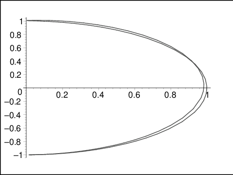
In the following, we analyze the error in the computation, by using Theorem 5. For this purpose, taking into account the assumptions introduced before Theorem 5, we consider . Thus, . Let be such that for every , it holds that
, and , for . We have that Then, by Theorem 5, we get that
and for every , it holds that
where .
In Figure 4, we plot curves and defined by and , respectively, for .
Figure 4: Curves and for
Example 3
Let , and the rational curve defined by the parametrization
Using the
SNAP package, one has that . We apply the algorithm and, in Step 1, we compute the polynomials
Now, we compute the polynomial . We have,
where
Then, (see Definition 1). Now, we apply Step 4 of the algorithm, and we consider
In Steps 5 and 6 of the algorithm, we determine the polynomials , and we compute the root in the variable of the polynomial . We get the rational parametrization . We simplify it, and we return the curve defined by the -numerical reparametrization
One may check that the equality of Theorem 2 does not hold. However, Remark 4 holds taking . Then, “ is an -proper reparametrization of ". In Figure 5, we plot the input curve and the output curve .
Figure 5: Input curve (left), curve (center), curves and (right)
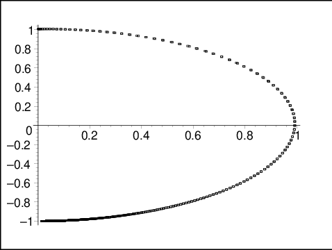
In the following, we analyze the error in the computation, by using Theorem 5. For this purpose, we consider . Thus, . Let be such that for every , it holds that
, and , for . We have that Then, by Theorem 5, we deduce that
and for every , it holds that
where , and .
In Figure 6, we plot curves and defined by and , respectively, for .
Figure 6: Curves and for
Example 4
Input Curve
Tolerance
Output Curve
Error bound
Figures
Curve
CurveCurvesand
Example 5
Input Curve
Tolerance
Output Curve
Error bound
Figures
Curve
CurveCurvesand
Example 6
Input Curve
,
Tolerance
Output Curve
Error bound
Figures
Curve
CurveCurvesand
6 Conclusion
The paper focus on the problem of numerical proper reparametrization which has both theoretical and practical background. Based on the results on the symbolic situation (see [17]), we achieve the expected properties and algorithm. For a given numerical curve, we can determine whether it is approximate improper with respect to a given precision and, in the affirmative case, an -proper reparametrization can be found. More important, the reparameterized curve obtained always lies in the certain offset region of the input one (and reciprocally). As a natural but more difficult problem, we would like to consider the problem of numerical proper reparametrization for rational space curves and surfaces.
References
[1] Abhyankar, S., Bajaj, C. (1988). Automatic Parametrization of Rational curves and Surfaces III: Algebraic Plane Curves. Computer Aided Geometric Design. Vol. 5, pp. 321–390.
[2] Arrondo, E., Sendra, J.,
Sendra, J.R. (1997). Parametric Generalized Offsets to
Hypersurfaces. J. Symbolic Computation. Vol. 23, pp. 267-285.
[3] Beckermann, B., Labahn, G. (1998). A fast and numerically stable Euclidean-like algorithm for detecting relatively prime numerical polynomials. Journal of Symbolic Computation. Vol. 26, pp. 691-714.
[4] Beckermann, B., Labahn, G. (1998). When are two numerical polynomials relatively prime? Journal of Symbolic Computation. Vol. 26, pp. 677-689.
[6] Corless, R.M., Giesbrecht, M.W., Kotsireas, I.S. van Hoeij, M., Watt, S.M. (2001).
Towards Factoring Bivariate Approximate Polynomials. Proc.
ISSAC 2001. pp. 85–92.
[7] Corless, R.M., Watt, S. M., Zhi, L. (2004). QR Factoring to compute the GCD of Univariate Approximate Polynomials. IEEE Transactions on Signal Processing. Vol. 52(12), pp. 3394–3402.
[8] Cox, D.A.,
Little, J., O’Shea, D. (1998). Using Algebraic Geometry. Graduate
Texts in Mathematics. Vol. 185. Springer–Verlag.
[9] Cox, D.A., Sederberg, T.W., Chen
F., (1998). The moving line ideal basis of planar rational
curves. Computer Aided Geometric Design. Vol. 8, pp. 803–827.
[10] Farouki, R.T., Rajan, V.T. (1988). On the numerical condition of algebraic curves and surfaces. 1: Implicit
equations. Computer Aided Geometric Design. Vol. 5, pp. 215-252.
[11]Galligo, A., Rupprech, D. (2002). Irreducible decomposition of curves. Journal of Symbolic Computation. Vol.33, pp. 661¨C677.
[12]
Gao, X.-S., Chou, S.-C. (1992). Implicitization of rational parametric equations. Journal of Symbolic Computation. Vol.14(5), pp. 459–470.
[13] Hoffmann, C.M., Sendra, J.R., Winkler, F. (1997).
Parametric Algebraic Curves and Applications. J. Symbolic
Computation. Vol. 23.
[14] Hoschek, J., Lasser, D. (1993). Fundamentals
of Computer Aided Geometric Design. A.K. Peters Wellesley MA.,
Ltd.
[15]Kaltofen, E., May, J.P., Yang, Z., Zhi, L. (2008). Approximate factorization of multivariate polynomials using singular value decomposition, Journal of Symbolic Computation, Vol.(43)5, pp. 359-376.
[16] Karmarkar, N., Lakshman, Y.N. (1996). Approximate polynomial greatest common divisors and nearest singular polynomials. ISSAC 1996, pp. 35-39. ACM Press.
[17] Pérez-Díaz, S. (2006).
On the Problem of Proper Reparametrization for Rational Curves and Surfaces. Computer Aided Geometric Design. Vol. 23(4), pp. 307-323.
[18] Pérez-Díaz, S., Schicho, J., Sendra, J.R. (2002).
Properness and inversion of rational parametrizations of
surfaces. Appl. Algebra Eng. Commun. Comput. Vol. 13(1), pp. 29–51.
[19] Pérez-Díaz, S., Sendra, J.R., Sendra, J. (2004).
Parametrizations of Approximate Algebraic Curves by Lines. Theoretical Computer Science on Algebraic - Numeric Algorithms. Vol. 315/2-3, pp. 627-650.
[20] Pérez-Díaz, S., Sendra, J.R., Sendra, J. (2005).
Parametrizations of Approximate Algebraic Surfaces by Lines. Computer Aided Geometric Design. Vol. 22(2). pp. 147-181.
[21] Pérez-Díaz, S., Sendra, J.R., Sendra, J. (2006).
Distance Bounds of e-Points on Hypersurfaces. Theoretical Computer Science. Vol 359. N. 1-3. pp. 344-368.
[22] Pérez-Díaz, S., Sendra, J.R., Villarino, C. (2007).
Finite Piecewise Polynomial Parametrization of Plane Rational Algebraic Curves. Applicable Algebra in Engineering, Communication and Computing. Vol 18(1-2), pp. 91-105.
[23] Pérez-Díaz, S., Rueda, S.L., Sendra, J.R., Sendra J. (2010).
Approximate parametrization of plane algebraic curves by linear systems of curves. Computer Aided Geometric Design. Vol 27. pp. 212-31.
[25] Sendra, J.R., Winkler, F. (2001). Tracing Index of Rational Curve Parametrizations.
Computer Aided Geometric Design. Vol. 18(8), pp. 771-795.
[26] Sendra, J.R., Winkler, F., Perez-Diaz, S. (2007). Rational Algebraic Curves: A Computer Algebra Approach. Series: Algorithms and Computation in Mathematics. Vol. 22. Springer Verlag.
[27]
Shen, L.-Y., Chionh, E.-W., Gao, X.-S., Li, J. (2011).
Proper reparametrization for inherently improper unirational varieties. Journal of Systems Sciences and Complexity. Vol. 24 (2), pp. 367-380.
[28] van Hoeij, M. (1994). Computing Parametrizations of Rational Algebraic Curves. In J. von zur Gathen (ed)
Proc. ISSAC 1994, pp. 187-190.
[29] van der Waerden, B.L. (1970). Algebra I and II.
Springer-Verlag, New York.
[30] van der Waerden, B.L. (1973). Einfürung in Die Algebraischen Geometrie. Springer Verlag, Berlin.
[31] Winkler, F. (1996). Polynomials Algorithms in Computer
Algebra. Wien New York: Springer-Verlag.
[32] Zeng, Z., Dayton, B.H. (2004). The approximate GCD of inexact polynomials part II: a multivariate algorithm. In Proc. ISSAC 2004. pp. 320-327.


![[Uncaptioned image]](1305.2461v2/ex51.png)
![[Uncaptioned image]](1305.2461v2/ex52.png)
![[Uncaptioned image]](1305.2461v2/ex53.png)
![[Uncaptioned image]](1305.2461v2/ex61.png)
![[Uncaptioned image]](1305.2461v2/ex62.png)
![[Uncaptioned image]](1305.2461v2/ex63.png)
![[Uncaptioned image]](1305.2461v2/ex71.png)
![[Uncaptioned image]](1305.2461v2/ex72.png)
![[Uncaptioned image]](1305.2461v2/ex73.png)