Molecular bands in extremely metal-poor stars

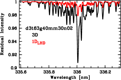
Using the downselected line list discussed in Sect. 2.1 and splitting the wavelength range in two parts we computed the full NH band. On the Paris cluster godot this took about 17 hours for each sub-band (computed in parallel), for 20 snapshots, 3 inclinations and 4 azimuth angles. The result is shown in Fig. 2 where the synthesis is compared with the one obtained from the corresponding $\mathrm{1D}_{\mathrm{LHD}}$ model. As expected the band is much stronger in the synthesis with the $\mathrm{CO}^{5}\mathrm{BOLD}$ model.

This computing time appears acceptable, each snapshot takes less than one hour. Parallelisation over snapshots should be able to provide the result in about one hour and parallelisation over angles in less than 10 minutes. These computational times approach what is achievable in one dimensional computations. With two important caveats: (i) the band is split in two sub-bands, parallelising also over 20 snapshots and 12 angle pairs implies $2\times 20\times 12=480$ processes; (ii) the overheads in accessing the snapshots and writing the results on disk should be carefully minimised by matching the procedure to the hardware capabilities of the system.

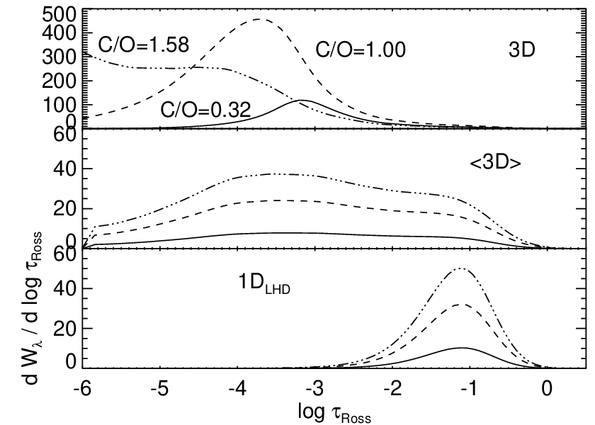
It is interesting to note that the $\mathrm{CO}^{5}\mathrm{BOLD}$ model is on average much cooler than the $\mathrm{1D}_{\mathrm{LHD}}$ model in the outer layers (see Fig. 3). Consistently the contribution function of the $\left\langle\mathrm{3D}\right\rangle$ model shows an extended tail in the outer layers. However the cooler mean temperature is not the dominant effect of the granulation. It is the horizontal temperature fluctuations that are responsible for the large difference between the NH band computed from the $\mathrm{CO}^{5}\mathrm{BOLD}$ model and from the corresponding $\mathrm{1D}_{\mathrm{LHD}}$ model. This can be appreciated by the large difference between the contribution function computed from the $\mathrm{CO}^{5}\mathrm{BOLD}$ model and that computed from the $\left\langle\mathrm{3D}\right\rangle$ model and from the corresponding differences in the computed bands (Fig. 3).

We should be cautious before claiming that real stars behave like this computation for two reasons:

1. 1.

   the temperature structure of the outer layers, where our computation puts the peak of the contribution function, could be radically difference in presence of a chromosphere;

2. 2.

   our computation has been carried out strictly in LTE, in the low-density outer layers we can expect non-equilibrium phenomena to play an important role. One should always remember the sobering result obtained for lithium (Cayrel & Steffen, 2000; Asplund et al., 2003), where indeed the NLTE effects lead to a totally different contribution function.

The recent observations of the 1083 nm He I line in metal-poor dwarf and subgiant stars by Takeda & Takada-Hidai (2011) suggest that, contrary to common wisdom and in spite of their old age, at least some of these stars possess chromospheres. It is therefore important to pursue both observational and theoretical studies in order to assess the role of chromospheres in metal-poor unevolved stars. The presence of a chromosphere may completely change the line formation of molecular bands and therefore the abundances deduced from their analysis. The $\mathrm{CO}^{5}\mathrm{BOLD}$ models have provided new insight in the solar chromosphere (Wedemeyer et al., 2004) suggesting that the temperature rise of the semiempirical chromospheric models (Fontenla et al., 1993, e.g.) likely traces only the clumps of hot material, in the presence of significant clumps of cold gas. This suggests that $\mathrm{CO}^{5}\mathrm{BOLD}$ extended models may be an important theoretical tool to investigate chromospheres in metal-poor stars.

It is equally important to pursue theoretically the computations of NLTE effects both on chemical equilibria and on molecular line formation.

The computation of the CN $B^{2}\Sigma^{+}-X^{2}\Sigma^{+}(0-0)$ violet 388.3 nm band is relatively easy to tackle. The line list computed by Plez et al. (2008) comprises 256 lines, thus we can compute it without splitting the range in smaller domains. Note that a CH line falls in the band and has to taken into account. The results are very different when using a $\mathrm{CO}^{5}\mathrm{BOLD}$ model or a $\mathrm{1D}_{\mathrm{LHD}}$ model. An example is shown in Fig. 4. The deduced nitrogen abundance, for a given observed spectrum, differs by more than a factor of 100.

This band provides a striking example of how the physics is different in a 3D hydrodynamical model atmosphere with respect to a corresponding 1D model atmosphere. The band is, a priori expected to depend on the oxygen abundance, however while in the 1D models, both $\mathrm{1D}_{\mathrm{LHD}}$ and $\left\langle\mathrm{3D}\right\rangle$, this results in a simple strengthening or weakening of the band, while the line formation depth remains more or less the same (see Fig. 5), when using the $\mathrm{CO}^{5}\mathrm{BOLD}$ hydrodynamic simulation, the line formation depth changes in a dramatic way, moving towards outer layers as the C/O ratio increases. The behaviour is indeed catastrophic when this ratio exceeds one: the contribution function would like to peak at optical depths smaller than those covered by the model. Clearly the synthesis in this case is not at all reliable, and should be taken only as an indication of the trend. It is questionable whether it is legitimate to extend the model at much lower optical depths that log($\tau_{Ross}$)=–6, where the presence of a chromosphere could already be felt and where the assumption of LTE is likely to break down. As pointed out in the case of the NH molecules, both the presence of chromosphere and NLTE effects could radically change this picture. It is nevertheless interesting to point out that the effects of the cool “clouds”, as captured by the $\mathrm{CO}^{5}\mathrm{BOLD}$ hydrodynamical simulation, gives rise to physical effects that are not predicted by any 1D model.

The G-band, the $A^{2}\Delta-X^{2}\Pi$ CH band, is challenging from the computational point of view, since it is very extended, and one wants to compute about 25 nm of synthetic spectrum. Moreover the observation that the ¹²C/¹³C ratios in metal-poor stars range from 3 to over 100, requires to keep track properly of both ¹²CH and ¹³C lines. Finally in such a large wavelength range the atomic lines cannot be neglected and also the wing of H$\gamma$. This implies that to synthesise the full band on needs to split the band in over 50 wavelength intervals, this calls for a large number of compute cores. For the time being we have just been able to synthesise the core of the band, as shown in Fig.  3 of Spite et al. (2013). For this computation we used a list of 99 lines, after a process of downselection, similar to what we described for NH above.