Giant magnetoresistance in the variable range hopping regime

In the localized regime the electron wave functions decay exponentially with the distance, $\mathbf{|r}-\mathbf{r}_{i}|,$ from the impurity:$\psi_{i}\left(\mathbf{r}\right)\sim\exp(-|\mathbf{r}-\mathbf{r}_{i}|/\xi)$ where $\mathbf{r}_{i}$ is the center of the localized wave function and $\xi$ is a typical localization radius. In this case the conductivity is determined by phonon assisted electron hopping between localized states. At low temperatures the typical hopping length $r_{hop}$ is determined by the competition between two exponential factors: the hopping probability $W_{ij}$ that decays exponentially with the distance between impurities $r_{ij}$ and the thermal factor, $\exp(-E_{hop}(r_{ij})/T)$ where $E_{hop}(r_{ij})$ is the hopping activation energy that decreases with $r_{ij}$. These factors give the exponential dependence of the typical hopping rate at distance $r_{hop}$: $\exp(-E_{hop}(r)/T-2r/\xi)$. This exponential factor is maximal for the typical hopping length, $r_{hop}$, which is much larger than the distance between localized states, as illustrated in Fig. 1b:

As a result, the resistivity acquires exponential dependence on temperature [2, 1]:

Here the prefactor $\rho_{0}$ is determined by the electron-phonon matrix element, $\xi$ is the localization radius.

Generally, the density of localized states can be energy dependent close to the Fermi energy [1]:

where we count the energy, $\epsilon$, of a tunneling electron from the Fermi energy. In the absence of electron-electron interaction (Mott’s theory) the density of states at the Fermi level is constant$\left(\beta=0,\,C=\nu_{0}\right)$ leading to activation energy $T_{0}\approx 13(\nu_{0}\xi^{2})^{-1}$ and exponent $\zeta=1/3$ for $d=2$ (Mott law). In the case when electrons (in 2D or 3D) interact via three dimensional Coulomb interaction (Efros-Shklovskii regime) $\beta=1$, $C\approx\left(2/\pi\right)e^{4}/\kappa^{2}$ , where $\kappa$ is the dielectric constant. This results in $\zeta=1/2$, $T_{0}\sim e^{2}/\kappa\xi$ for 2D electrons interacting via three dimensional Coulomb.

The qualitative arguments of the Mott theory can be made more quantitative by considering the optimal percolating cluster of electron hops.[1] Probability of a single hop between the states localized around positions $r_{i}$ and $r_{j}$ is given by

Here

is the phonon matrix element, $u$ is the speed of the sound and $\overrightarrow{q}$ is its wave vector. Because the wave functions $\psi_{i}(\vec{r}-\overrightarrow{r}_{i})$ and $\psi_{j}(\vec{r}-\overrightarrow{r}_{j})$ decrease exponentially, $M_{ij}$ and $W_{ij}$ are exponential functions of the localization length, $\xi\left(B\right)$.

In the main part of our paper we consider the range of magnetic field in which $W_{ij}(B)$ dependence is dominated by $\xi\left(B\right)$. In this case one can approximate the phonon tunneling matrix element by the amplitude of tunneling between states $i$ and $j$: $M_{ij}\sim A_{ij}$.

In the uniform medium the magnetic field suppresses the amplitude of a single quantum tunneling event:

which gives positive magnetoresistance. Here $L_{B}=\left(c\hbar/eB\right)^{1/2}$is the magnetic length. In disordered media, electrons scatter from other localized states which have energies different from the energy of the final state. The effect of magnetic field is due to the interference of the directed optimal paths, which is shown schematically in Fig. 1b. In this case $A_{if}=\sum_{\Gamma}A_{\Gamma}$ is a coherent sum of amplitudes, $A_{\Gamma}(B)$, to tunnel along paths $\Gamma$, between the initial "i" and final "f" sites. The tunneling paths can be defined by the sequence of states which scatter electrons in the course of tunneling. At zero magnetic field $\textbf{B}=0$ the wave functions of localized states and the tunneling amplitudes $A_{\Gamma}(0)$ can be chosen to be real: [30]

Here $\mu{}_{\alpha}$ is the amplitude of scattering on $\alpha$’s localized state, $\epsilon_{i}$ and $\epsilon_{\alpha}$ are energies of the tunneling electron and the localized scattering state, $b\sim\sqrt{\xi}\epsilon_{0}>0$, and $\epsilon_{0}$ is the characteristic binding energy of the localized states. Generally $\epsilon_{\alpha}$ are random quantities, so the amplitudes $A_{\Gamma}(\textbf{B}=0)=A_{\Gamma}(0)$ have random signs. Note that the equation (7) describes both the processes in which an electron is scattered by empty sites and the ones in which it goes through the occupied sites (see Fig. 2) which can be described as a hole moving backwards. The important condition for the interference is that in the final state all intermediate electrons should return to their original positions and spin states.

The hopping probability $W_{if}$ is a random quantity. Generally, to get the value of the resistance of the system one has to solve the full percolation problem with the probability of individual hops given by $W_{if}$.[1] However, as long as $\ln[\rho(B)/\rho(0)]/\ln\rho(0)\ll 1$ the magnetoresistance is given by the average of the logarithm of the hopping probability[1]:

Here the brackets denote averaging over random scattering configurations and over different hoppings which belong to a percolation cluster. These hoppings are characterized by a typical hopping length, $r_{hop}$. With a good accuracy, one can replace the full average (10) with the average over random scattering configurations for the hopping processes by the distance $r_{hop}.$ Physically the averaging of the logarithm in (10) means that the resistivity is controlled by the typical hopping probability, rather than by rare events.

The application of a magnetic field B introduces random phases to the tunneling amplitudes

where $\Phi_{\Gamma}=BS_{\Gamma}$, $S_{\Gamma}$ is the area enclosed between the path $\Gamma$ and straight line going from initial to final states, see Fig. 1b.

Depending on distributions of the signs of the amplitudes $A_{\Gamma}(0)$ the orbital magnetoresistance can be both positive and negative. To illustrate this fact let us consider a model in which there are only two paths, $A_{1}(0)\sim A_{2}(0)$, which are independent random quantities and $|\Phi_{1}-\Phi_{2}|\sim\Phi_{0}$. If $A_{1,2}(0)>0$ are positive, in the presence of magnetic field, the amplitudes $A_{\Gamma}(B)$ partially cancel each other. As a result, $\langle\ln W_{ij}(B)\rangle$ decreases by a factor of the order of one when $|\Phi_{1}-\Phi_{2}|\sim\Phi_{0}$. In this case the magnetoresistance is positive.

The situation changes if $A_{1,2}(0)$ have random signs. In the simplest case when the signs are completely random, the average probability $\left\langle\left|\sum A_{\Gamma}(B)\right|{}^{2}\right\rangle=\sum\left\langle\left|A(0)\right|^{2}\right\rangle$ is independent of B. If magnetic flux through the closed loop formed by paths $1$ and $2$ is larger than the flux quantum, the phases of the amplitudes $A_{1,2}$ are completely random, so that $\left\langle A_{1}(B)A_{2}(B)\right\rangle=0.$ This implies that the variance $\left\langle\left|\sum_{\Gamma}A_{\Gamma}(B)\right|{}^{4}\right\rangle-\left\langle\left|\sum_{\Gamma}A_{\Gamma}(B)\right|^{2}\right\rangle^{2}$ decreases by a factor of the order of one when $|\Phi_{1}-\Phi_{2}|\sim\Phi_{0}$. As a result, a typical value of $W_{if}$ defined by (10) increases by a factor of the order of one and the magnetoresistance is negative.

This simplified picture of magnetoresistance being determined by the interference between two paths becomes more complicated for two reasons. First, at large scales the propagation amplitude is dominated by many paths which go through the same scatterer or a group of scatterers. This implies strong correlations between amplitudes $A_{\Gamma}$ , as we discuss in section III.1. This makes the mathematical problem of calculation of $\rho(B)$ non-trivial. Second, the behavior of the magnetoresistance becomes more complicated if amplitude signs are correlated at some finite distances (see section II.3). In this case, one expects a crossover from the negative to positive magnetoresistance as the field is increased, as we explain in section III.

Because the sign and the magnitude of the magnetoresistance are intimately related to the statistics of sign and amplitude distribution of $A_{ij}(0)$ we start with a discussion of this quantity.

In the case of small and positive scattering amplitudes, $\mu_{\alpha}>0$, and at zero magnetic field the problem of electron tunneling can be mapped [31, 32, 33, 30] onto the problem of directed polymers. In the latter problem one studies the thermodynamics of an elastic string in a delta-correlated two dimensional random potential, $W(x,y)$ that is characterized by energy functional

Introducing the partition function, $Z(y,x)=\sum_{y\{x\}}\exp(-\beta H)$ of the string that ends at point $(x,y)$ one gets that its evolution as a function of $x$ is described by the equation

This equation should be compared with the equation for the particle propagation in disordered media:

with white noise potential $V(x,y)$. At negative energies corresponding to tunneling we substitute $\Psi=\exp(-\beta\sigma x)Z(x,y)$; one can neglect second order derivative in $x$ terms that are small at weak potential $V\ll-E$. Then, the Schrodinger equation (14) coincides with (13) with $(\sigma\beta)^{2}=-2mE$ and $W=\sigma V/2E$. This mapping also holds for arbitrary (not necessarily white noise correlated) potential $V$. However, it becomes less useful for arbitrary potentials because analytical results for this problem were obtained only in the case of the white noise potential.

Computation of positive magnetoresistance requires the solution of the directed polymers beyond the white noise approximation, so the analytical results are not directly applicable. Furthermore, the physically relevant problem of scattering with negative amplitudes cannot be mapped onto any thermodynamic problem because the corresponding free energy becomes imaginary. The applicability of the results of the directed polymer problem in the white noise approximation becomes even more questionable in this case. Below we give a brief review of the results of the direct polymers problem in the white noise approximation. Then we present results of our numerical simulations beyond the white noise approximation, which indicate that these problems belong to the same universality class. Finally, we discuss the statistics of the signs of the tunneling amplitude and show that the existence of the “sign phase transition” is compatible with the results for directed polymer problem.

The main result of the directed polymer theory is the scaling form of the fluctuational part of the free energy of the polymer of length $L$, $F\propto L^{1/3}$and its deviations in the transverse direction $Y\propto L^{2/3}.$ For equivalent problem of domain wall pinning this scaling was first found numerically in work[34]. Analytically, it was extracted from the third moment of the distribution function of polymers of length $L$, ${\cal{P}}(F)$.[35, 36] The replica method that was used in this work might be questioned because of an apparent non-commutativity of the limits $L\rightarrow\infty$ and $n\rightarrow 0$ and because it gives unphysical results for all moments of the distribution function except the third. All these problems can be eliminated by solving for the distribution of the energy differences of the infinitely long polymers that end at different points $y_{1},y_{2}$, this solution gives the same scaling exponents. [37] as the original approach[34, 38, 39, 40, 35, 36].

The striking generality of this scaling result that we prove by numerical simulations below is, probably, due to the qualitative reasoning that relates it to the Markovian form of the free energy fluctuations as a function of transverse coordinate. Indeed, The Markovian form implies that free energy fluctuations at large scales are proportional to $Y^{1/2},$ on the other hand they should be of the order of the string elastic energy at these scales: $Y^{2}/L\propto Y^{1/2}$. Solving the last equation for $Y$ we get the scaling dependencies of the exact solution and of the numerical simulations.

Despite being intuitively appealing, the Markovian nature of free energy fluctuations is difficult to prove for the physically relevant situation in which some scattering amplitudes (9) are very large. It is even more difficult to prove it for the case of rare negative scattering amplitudes in which wave function can change sign at some points. At these points the free energy defined by $F\equiv-T\ln Z$ acquires imaginary part ($\Im F=\pi$) whilst its real part becomes large. Because these points are due to close by negative scatterers, the effective free energy becomes highly correlated which violates the main assumption of the Markovian nature of the free energy fluctuations.

Recently[41, 42], a full Bethe ansatz solution of problem (12) established the complete form of the distribution function of free energy $F\equiv-T\ln Z$ of the string of length $L$, which turns out to coincide with the Tracy-Widom distribution[43]. This result allows one to check if the problem of particle hopping belongs to the same universality class as the directed polymers. Namely, we define the effective free energy of the quantum problem as

where $A$ is the electron amplitude at site $(x,y)$ propagating in $x$-direction. This free energy describes the decay of the wave function. We compute the amplitude $A$ by simulating electron propagation and check the scaling properties of its real part fluctuations in $y$-direction and the universality of the distribution function.

We determine the amplitude $A$ from the solution of the lattice recursive equation

where $\epsilon_{ij}$ are random independent variables defined on each lattice site and $g$ is the parameter that determines the average decay of the amplitude (inverse localization length). We shall discuss below different distribution functions of $\epsilon_{ij}$ appropriate for different physical systems.

Physically, the model (16) describes the motion of electrons on the lattice shown in Fig. 3. The site with energy $\epsilon_{ij}=\left\langle\epsilon\right\rangle$ can be identified with ideal lattice, the rest with impurities. If energy $\epsilon_{ij}$ is distributed in a narrow interval around its average, the evolution (16) becomes equivalent to (14) in the continium limit. As discussed in section II.1 the most physically natural choices of the distribution function of $\epsilon$ are uniform $P(\epsilon)=\theta(\epsilon)$, linear $P(\epsilon)=2\epsilon$ and their analogs for the negative scattering amplitudes: $P(\epsilon)=1/2$, linear $P(\epsilon)=|\epsilon|$. In all cases we assume that the distribution is cutoff by $\epsilon_{0}$ at large $\epsilon$: $P(|\epsilon|>\epsilon_{0})=0$. The choice of $\epsilon_{0}$ determines the average decay rate of the electron amplitude which is mostly irrelevant, in the computations we have set it to $\epsilon_{0}=1$. We have also studied the gapped distribution $P(\epsilon)=2$ for $1/2<\epsilon<1$ for which we expect to get the results similar to the one predicted by exact solution. Finally we studied the binary distribution $P(\epsilon)=(1-X)\delta(\epsilon-1)+X\delta(\epsilon-(\mu+1)^{-1})$ characterized by parameter $X$ and negative scattering amplitude $\mu<0$.

Some of our results are presented in Figs. 4 and 5. For all studied distribution we observe very good scaling, $\left\langle\Delta F^{2}\right\rangle^{1/2}\propto L^{\gamma}$, with the exponents $\gamma=0.28,\,0.345,\,0.343$ for gapped, linear and uniform densities of states respectively. These values are very close to the expected value $1/3$, especially for the linear and uniform densities of states. The data for the gapped density of states display a significant transient regime, so the deviation of the exponent from the analytical result is not surprising. The presence of negative scattering amplitudes has small effect on these exponents, they become $\gamma=0.31,\,0.33,\,0.345$ that are even closer to the expected values. Furthermore, the higher moments of the distribution function tend to the universal values expected for the Tracy-Widom distribution. These results is in agreement with the works[44, 45] that observed Tracy Widom distribution of conductances in two dimensional models.

These data lead to the conclusion that the main results of the directed polymer problem, namely, the scaling dependence of the free energy and the universality of the distribution function remain valid for the problem of electron tunneling in disordered media.

As explained in section II.1, the sign of the magnetoresistance is related to the statistics of signs of amplitudes $A_{if}(0)$ in the absence of magnetic field. If the concentration of impurities with negative scattering amplitudes is large, the sign of $A_{if}(0)$ becomes completely random. If all impurities are characterized by positive scattering amplitudes $\mu_{i}>0$, the sign of $A_{if}(0)$ is positive. Let us denote the probability to find a positive amplitude $A_{if}(0)$ by $P_{+}$ and negative by $P_{-}.$ The quantity $\Delta P=P_{+}-P_{-}$characterizes the sign order. As the concentration, $X$, of the impurities with negative scattering amplitudes increases, $\Delta P$ should change from $1$ to $0$. Generally, $\Delta P$ is scale dependent and acquires its limiting value at $|r_{i}-r_{f}|\rightarrow\infty$. There are two logical possibilities: either at large scales $\Delta P_{r\rightarrow\infty}=0$ only for $X>X_{c}$ while for smaller $X<X_{c}$ $\Delta P_{r\rightarrow\infty}>0$ , or that any non-zero $x>0$ leads to $\Delta P_{r\rightarrow\infty}=0$. The former implies that the change in the $x$-dependence of the sign statistics can be viewed as a phase transition. This possibility has been suggested in [24, 25, 27], the alternative was argued for in works [31, 32, 33].

Here we study the sign statistics in the lattice models defined by (16) in section II.2 and show that both the phase transition and crossover can be realized depending on the distribution of $\epsilon.$ We start with the simplest case of binary distribution $P(\epsilon)=(1-X)\delta(\epsilon-1)+X\delta(\epsilon+\epsilon_{0})$ with small $X\ll 1$ and small $\epsilon_{0}\ll 1$. This model describes the wave function propagation on the ideal lattice (sites with $\epsilon=1$) which contains rare impurities characterized by a negative scattering amplitude $\mu\approx-1/2\epsilon_{0,}|\mu|\gg 1$. The large value of $|\mu|$ allows a continuous description of the tunneling amplitude. The size of the region where the tunneling amplitude $A_{if}(0)<0$ is negative may be found by noticing that the wave function

changes its sign in the egg-shaped region in the wake of the impurity given by:

The area of this region is

A small concentration, $XS\ll 1$ of such impurities leads to independent lakes of negative signs shown in Fig. 6. In this situation $\Delta P>0$ .

As the concentration $x$ is increased, different lakes start to overlap and form a state with random sign of the amplitudes. The transition between these two phases takes place at $X=X_{c}\sim{\it S}^{-1}\propto|\mu|^{-3}$. The dependence $P_{-}(X)$ is expected to have a general form characteristic of a phase transition sketched in Fig. 7a. These qualitative arguments ignore the contributions from impurities located close to each other which should not be relevant in the limit $X\rightarrow 0$.

The numerical simulations show that the transition survives for not so large values of the scattering amplitudes as well. In particular, this has been observed for the binary distribution functions with $\epsilon_{0}=1$. Fig. 7 represents the results of our numerical simulations for this case. As one can see, the behavior of $\Delta P$ as a function of the distance changes qualitatively as one increases $X$  beyond $X_{c}\approx 0.032$. For smaller concentrations, $x$, probability difference $\Delta P$ saturates at non-zero values, whilst for larger concentrations it approaches $0$. The scales needed to observe this change in the behavior are generally very long. We believe that this is the reason that prevented establishing unambiguously the existence of the transition in early numerical simulations. We note that the scales are further enlarged near $X_{c}\approx 0.032$ as one expects at a phase transition.

We have also checked that the phase transition between the sign ordered and sign disordered phases survives for a gapped distribution of $\epsilon$ defined in section II.2. The numerical data look very similar to those shown in Fig. 7, the expected value of $X_{c}$ in this model is $X_{c}\approx 0.02$.

The existence of the sign phase transition has been questioned in paper [33] which used the mapping to the directed polymer problem. The essence of the argument is that the free energy of directed polymers leading to a given site are dominated by a single path, so that just a single impurity along this path suffices to change the sign of the amplitude. At a small concentration of negative scatterings, one concludes that the amplitude should become completely random at the scale $L\propto 1/X$. This argument, however, does not take into account the contribution from subdominant paths that may eventually restore the sign of the amplitude at large scales as is indicated by numerical data for the gapped density of states, see section II.2.

We now show that for a gapless density of states (3) with $\beta<2$ and for any non-zero concentration of negative scatterers the sign of the amplitude $A$ becomes completely random at large scales. Indeed, in this case the total area of negative lakes is

where $S\left[\mu\right]\propto\mu^{3}\propto\varepsilon^{-3}$. Thus, $S_{tot}$ diverges for all densities of states $\nu\left(\epsilon\right)\sim\varepsilon^{\beta}$ with $\beta\leq 2$. This is the case for example in the case of Coulomb gap where $\nu\left(\epsilon\right)\propto\varepsilon$.

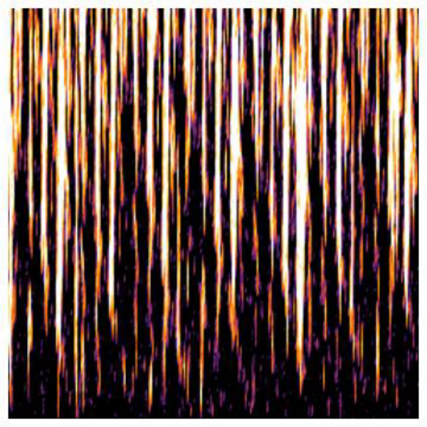
We have checked this conclusion numerically for the linear density of states and we have indeed observed that even a very small $X\sim 10^{-4}$ leads to a random sign of the amplitude at very large scales. Our data are shown in Fig. 8. As one expects, the scale at which the sign becomes random grows quickly with the decrease of $X$.

We now turn to the discussion of magnetoresistance in the variable hopping regime. We begin by summarizing the results of numerical simulations for the recursive equation (16) that was modified to include the phases, $\phi_{j}=Bj$, induced by magnetic field

Then we give the qualitative explanation of the results based on the mapping to the directed polymer problem. The dimensionless magnetic field $B$ in this equation and in the discussion below is given by the flux of the physical magnetic field, $B_{phys}$, through the elementary square Malplaquet of the lattice: $B=B_{phys}a^{2}/\Phi_{0}$ where $a$ is the lattice constant and $\Phi_{0}=hc/e$ is the flux quantum.

Our main result is that at large $r_{hop}>L_{B}$ (which holds at low temperatures), both positive and the negative magneto resistances are described by corrections to the localization length:

This scaling law is characterized by the universal exponent $\alpha\approx 4/5$ and non-universal numerical coefficients $C_{\pm}$. The latter depends on the distribution of $\varepsilon_{ij}$, e.g. $C_{+}\approx 2.6$ for the gaped and $C_{+}\approx 0.9$ for linear density of states. Here we define the localization length as the limiting behavior of the amplitude $\xi=\lim_{r_{ij}\rightarrow\infty}\ln A_{ij}(B)/r_{ij}$. The positive sign ($+$) in (18) corresponds to the case where the system is in the sign disordered phase, the negative sign corresponds to the sign ordered phase. The universal regime (18) is achieved at low fields. Notice that whilst the value of $\xi(B)$ is mathematically defined for any magnetic field, its applicability to the hopping problem requires that $r_{hop}>l_{B}$.

At intermediate fields one often observes a slightly different power law

with a different exponent and pref actors, $\alpha^{\prime}\approx 0.5,\,0.6,\,0.64$ for the scattering of random signs with gaped, linear and uniform densities of states respectively. For these densities of states the pref actors are $D_{+}\approx 0.11,\,0.22,\,0.30$. The value of $D_{+}$ for the gaped density of states is in agreement with the numerical simulations of the previous workers [26, 28]. Note that the value of $D_{+}$ for the uniform density of states is roughly three times larger that for the gapped one. This makes it possible to observe large negative magnetoresistance experimentally as we discuss in section V. These statements are illustrated in Figs. 9. The scaling dependence with the exponent $\alpha^{\prime}\approx 0.6$ was observed previously in a number of works[32, 28] in which insufficient system sizes prevented the observation of the asymptotic behavior.

We now give qualitative arguments that reproduce the observed scaling behavior of the change in the localization length explained above.

As we have shown in section II.2, the problem of electron tunneling belongs to the same universality class as the problem of directed polymers. In particular, the typical tunneling action varies from one path to another by the amount that scales as $\Delta F\propto L^{1/3}.$ This means that the tunneling from point $i$ to $f$ is dominated by a narrow bundle of paths as shown in Fig. 10. The width of this bundle does not increase with the length of the path, so the magnetic field has very little effect on the tunneling in this approximation. Another bundle of paths that differs from the dominant one at scale $L$ has action that is typically larger than that of the dominant path by $\Delta F\propto L^{1/3}$, so its amplitude is exponentially suppressed by $\exp\left[-c(L/a)^{1/3}\right]$. Here $a$ is the mean free path of the electron (lattice spacing in the case of numerical simulations). This leads to an exponentially small effect of magnetic field. However, because the difference of the actions between two paths is a random variable itself, with probability $p\propto L^{-1/3}$ two actions differ only by the amount of the order of unity. If all scattering amplitudes are positive, the change in the interference caused by magnetic field decreases the total amplitude by the factor of the order of unity, provided that the flux through the loop formed by these two paths is of the order of the flux quantum. Because the transverse direction scales as $Y\sim a(L/a)^{2/3}$ the interference becomes relevant at scales

with probability $p\sim(L/a)^{-1/3}.$ The resulting decrease of the wave function implies that the typical inverse correlation length increases by

Repeating the same arguments for the case of the amplitudes of the random signs and using the fact that the signs of two paths that contribute to the interference are random (cf. discussion after equation (11)), we get the same dependence on magnetic field but with the opposite sign: the inverse correlation length is decreased by magnetic field.

All these conclusions are valid in the limit of long scales where $\Delta F\gg 1$. In the intermediate regime, in which $\Delta F\lesssim 1$ the probability that two paths interfere is of the order of unity resulting in the scaling dependence of $\delta\xi^{-1}$on the field with the exponent $\alpha^{\prime}=3/5$. Looking at the numerical results for the scaling dependence of $\Delta F$ shown in Fig. 4 we see that it remains of the order of unity for $L\lesssim 10^{2}$ which translates into the field $B\gtrsim 10^{-3}$ in rough agreement with the numerical results shown in Fig. 9.

The behavior of the correlation length is given by the simple scaling equations (18,19) only in the limit of completely random and positive amplitude signs. In the case of a small concentration of negative scatterings one expects a more complicated behavior. Large fields affect amplitude at short scales. At these scales the rare negative scatterings have small effect on the amplitude sign, so at large fields the inverse localization length is increased by the field, similarly to the case of positive scattering amplitudes. In contrast, at large scales relevant for small fields the amplitude sign becomes completely random, so at small fields one expects a negative correction to $\delta\xi^{-1},$ similar to a fully random sign case. As the field is increased, the sign of the correction should change. Exactly this qualitative behavior is shown by numerical simulations of the model (17) with a small concentration of scatterers with negative amplitudes. Our results shown in Fig. 11 display universal behavior of $\delta\xi^{-1}(B/B_{0})$. The characteristic field $B_{0}$ scales, as expected, with concentration $X$: $B_{0}\propto X^{\beta}$, however, the value of exponent $\beta\approx 2.8$ is sufficiently larger than one would expect from the scaling behavior of $L(x)\propto 1/x$ obtained in section II.3: $\beta_{expected}\approx 1.6$. We do not have a satisfactory explanation of this discrepancy. We only note that very small values of $B_{0}$ found numerically imply that even a small amount of sign correlations is sufficient to result in the positive $\delta\xi^{-1}$. This is not so surprising because positive increment of $\delta\xi^{-1}$, although given by the same scaling dependence, is order of magnitude larger than the negative one (cf. right and left panels of Fig. 9).

The scaling dependence (18) is non-analytic in $B$, so it should dominate over other sources of corrections to the localization radius at $B\rightarrow 0$. In the electron hopping problem the largest scale, $r_{hop}$, for the coherent electron tunneling is set by temperature (1). The non-analytic behavior predicted by (18) takes place provided that the scale $L$ given by (20) is less than $r_{hop}(T)$:

In the discussion of the hopping transport we have assumed the strongly localized regime in which the electron wave function is localized at the scales of the order of the Bohr radius, $a_{B}$ of a single impurity. However, all our qualitative conclusions should also hold when localization length is larger, $\xi>a_{B}.$ In this case the electrons tunnel from one area to another as shown in Fig. 12. The loops of the tunneling paths are allowed inside individual areas, but not between them. In this regime one expects to observe large non-analytic dependence of the localization length on magnetic field given by (18,19) at low fields $B\xi^{2}\lesssim\Phi_{0}$. These universal corrections adds to the effect of magnetic field coming from the scales shorter than $\xi$ that may be found from the renormalization group approach. These corrections are of the order of $\delta\xi/\xi\sim(B\xi^{2}/\Phi_{0})^{2}$ and thus are negligible compared to the effects (18,19) coming from the longer scales at low fields. They can, however, contribute significantly to the total variation of the magnetoresistance at large fields.

The results (18,19) for the $\xi(B)$ dependence can be converted into magnetoresistance provided that the induced change of the localization length is small $\delta\xi\ll\xi,$ but the resulting change in the hopping amplitude is exponentially large leading to resistance variations $\ln\left(\rho\left(0\right)/\rho\left(B\right)\right)\gg 1$. In this case one can neglect other contributions to the variation of the hopping probability (that we discuss below) so that magnetoresistance is given by

Combined with the $\xi(B)$ dependence discussed in section III.1 this equation gives the magnetoresistance at moderate fields, so that $B\xi^{2}\lesssim\Phi_{0}$ but $\ln\left(\rho\left(0\right)/\rho\left(B\right)\right)\gg 1$.

At large magnetic fields $B\xi^{2}\gtrsim\Phi_{0}$ the equation (21) remains valid but the localization length dependence on magnetic field is due to short scales and is non-universal. For a granular metal the localization length is roughly equal to the grains size $r_{0}$; because the magnetic field has no effect at scales shorter than $r_{0}$, $\delta\xi(B)$ dependence saturates at $B\xi^{2}\lesssim\Phi_{0}$. In contrast, in the case of a weakly disordered non-interacting 2D metal with $kl_{tr}$>1 one expects[7] strong dependence on magnetic field. Indeed, in this case the localization length is exponentially large $\xi\left(0\right)\sim l_{tr}\exp\left(k_{F}l_{tr}\right)$ in the absence of magnetic field, $l_{tr}$ being electron mean free path. The conventional renormalization group analysis[7] gives $\delta\xi(B)/\xi(0)\sim(B\xi^{2}/\Phi_{0})^{2}$ at $B\xi^{2}<\Phi_{0}$, so one expects corrections of the order of unity at $B\xi^{2}\approx\Phi_{0}$. At larger fields ($Bl_{tr}^{2}\sim\Phi_{0}$) the localization length increases exponentially to $\xi(B)\sim l_{tr}\exp\left(k_{F}l_{tr}\right)^{2}$. At even larger fields one expects the appearance of the quantum Hall regime and a pseudometallic behavior.[13] The presence of electron-electron interaction can lead to even larger variety in the localization length dependence on magnetic field at high fields.

The computation of $\xi(B)$ dependence in section III.1 translates into the predictions for magnetoresistance (21) only in the asymptotic regime of large magnetic field at which $\ln\left(\rho\left(0\right)/\rho\left(B\right)\right)\gg 1$. There are at least two reasons why it is important to study the magnetoresistance in the opposite limit of low magnetic field.

First, because it is difficult to measure large resistances, the parameter $r/\xi\lesssim 15$ cannot be very large, so the condition is $\ln\left(\rho\left(0\right)/\rho\left(B\right)\right)\gg 1$ is satisfied only in a limited range of fields. As we show below, the power law dependence of $\ln\left(\rho\left(0\right)/\rho\left(B\right)\right)$ extends somewhat in the regime if $\ln\left(\rho\left(0\right)/\rho\left(B\right))\right)\lesssim 1$ which makes the observation of this dependence more realistic.

Second, many data show that the magnetoresistance often changes sign in small fields. As we discuss in more detail below, this sign change agrees with the theoretical expectations. For instance, if the scattering amplitudes are mostly positive ($P_{-}\ll 1$) the localization length at large fields becomes shorter (see section II.3) and magnetoresistance is positive. However, at small fields it may change its sign and become negative. This change in the sign of the magnetoresistance can be due to the change in the sign of the correction to the localization length discussed in section II.3or to another effect at short scales that we discuss below. Generally, the theoretical predictions in this regime are less universal.

At small magnetic field the accuracy of the approximation $M_{ij}\sim A_{ij}$ becomes insufficient because it overestimates contributions to the hopping rate (4) from the impurity configurations in which the partial amplitudes $A_{\Gamma}\left(0\right)$cancel each other in the absence of magnetic field, so that the value of $A_{if}(0)\approx 0$. For these configurations a small magnetic field changes $\ln A_{if}$ dramatically. For a finite probability density of $A_{ij}(0)=0$ the magnetic field dependence of $\overline{\ln A(B)}$ becomes a non-analytic function of $B$: $\overline{\ln\left[A(B)/A(0)\right]}\propto|B|$. [24, 25] Similarly to the qualitative discussion of $\xi(B)$ dependence in section III.1 this non-analyticity can be demonstrated in the case when propagation amplitude is due to the interference between just two paths: $A_{if}=A_{1}+A_{2}\approx 0$ with random $A_{1}$and $A_{2}$. In this model case the typical amplitude in magnetic field becomes

where $\phi\propto B$ is the phase difference induced by the magnetic field. Here and below we denote by bar the averaging over the impurity configurations. Because the probability density of $A_{ij}(0)=0$ is finite at any concentration of scatterers with $\mu_{i}<0$, the typical amplitude always grows at small fields. This however does not always translate into negative magnetoresistance.

The crucial difference between the amplitude $A_{ij}$ and the hopping rate (4) is that the latter is the sum of the positive rates due to phonons with different $q$ directions. As a result, the probability density to find $W_{if}=0$ is zero, and at small $B$ the magnetorsistance is proportional to $B^{2}$.

In order to find the values of the crossover fields we note that in the limit of low temperatures at which $qr_{ij}\ll 1$ the exponential in (5) can be approximated by the first non-zero term:

The main contribution to the matrix element $M_{ij}$ comes from the components of the phonon wave vector $\overrightarrow{q}$ which is parallel to $\vec{r}_{ij}$. In the leading approximation we can neglect the contributions from the phonons with momenta in other directions. In this approximation the hopping probability (4) is controlled by the matrix element $M_{ij}(q\hat{r}_{ij})$ $\hat{r}_{ij}=\overrightarrow{r_{ij}}/r_{ij}$. This matrix element has the same statistical properties as the amplitude $A_{if}$, so the reasoning resulting in (22) applies and $\overline{\ln\left|M\left(B,\overrightarrow{q}\right)/M\left(0,\overrightarrow{q}\right)\right|}\sim\left|B\right|$. The subleading processes in which the hopping (4) is due to phonons with momenta perpendicular to $\vec{r}_{ij}$ cut off the non-analytic behavior of $\overline{\ln W(B)}$ at very small fields.

Combining this result with the effect of $\xi(B)$ dependence discussed in section III.1 that takes place at large scales at which the flux through the typical loop is larger than the flux quantum, $Br^{5/3}\xi^{1/3}>\Phi_{0}$, we get three regimes of the $\overline{\ln M(B)}$ dependence for $B\xi^{2}<\Phi_{0}$:

where $B_{0}=\Phi_{0}/r^{5/3}\xi^{1/3}.$ As we saw in section III.1 the transverse deviations of the typical path scale as $r_{\perp}\sim r^{2/3}\xi^{1/3}$. This allows us to estimate the contribution to the average (4) from phonons with $q\perp r$: $W_{\perp}\sim(\xi/r)^{2/3}W$. Repeating the arguments that led to (22) we get

that results in the dependence (25) with $B_{*}=\Phi_{0}/r^{2}$.

The qualitative estimates show that while the regime of non-analytic dependence is relatively wide ($B_{0}<B<\Phi_{0}/r^{2})$ the regime of the linear dependence is narrow. We note that the estimates of $B_{*}$and $B_{0}$ neglect the numerical coefficients that might be important.

The discussion above and the result (24) assumed that the system is deep in the sign disordered phase in which signs of all amplitudes are completely random. If the scattering amplitudes are mostly positive $P_{-}\ll 1$ the signs of the amplitudes become random only at large scales. It implies that the system may be in the sign ordered phase at characteristic scales set by magnetic field. In this case the magnetoresistance at largest fields is positive in contrast to (24), while at small $B$ it is quadratic in $B,$ so it can be both positive and negative depending on the value of $P_{-}\ll 1$.

To check the validity of (25) for realistic parameters we have performed the numerical computation of the matrix elements. We did not attempt a full computation of the matrix element and its averaging over the distribution of $r_{ij}$ that characterize the percolating cluster. Instead, we computed matrix element for the characteristic $r_{ij}$ and averaged over different direction of $q$. Because the results do not change qualitatively when $r$ is increased by a factor of $2$, we believe that they reproduce faithfully the dependence of the magnetoresistance:

where angular brackets denote averaging of the directions of $\vec{q}$. The result of our numerical simulations for the case of uniform density of states $P(\epsilon)=(1/2)\theta(1-|\epsilon|)$ is shown in Fig. 13 for two typical distances: $r/\xi\approx 8$ and $r/\xi\approx 6$. In both cases one observes a large regime of the pseudo-universal behavior $\ln(\rho(0)/\rho(B))\sim B^{\alpha}$ with $\alpha\approx 0.5$ that is due to the non-universal corrections to the localization length (19). At larger $r/\xi\gtrsim 8$ one observes the gradual appearance of the transient linear dependence in magnetic field in agreement with the expectations (25). Figure 14 shows expected magnetoconductance at different typical values of $r/\xi$ converted into expected values of the resistances.

So far in our discussion we have ignored the many body effects due to electron-electron interaction. Generally one expects that electron correlations play much bigger role in the hopping regime than in the metallic regime. In this subsection we briefly discuss their role, and the conditions under which the single particle results obtained above are valid.

At low temperatures the electron sites with $\epsilon_{\alpha}<0$, (and $\mu_{\alpha}<0$), are occupied by electrons, while the sites with $\epsilon_{\alpha}>0$ are empty. Tunneling between initial and final states may be viewed as a virtual process in which the electron hops through the intermediate localized states. Depending on the ratio between the electron-electron interaction and the density of states at the Fermi energy in the impurity band, these localized states can be singly and doubly occupied. The spins in the singly occupied states interact via the exchange interaction, $J$. Although the detailed theory of the disordered electron systems does not exit, three obvious limiting cases are clearly possible. In the first case, the interaction between electrons is large, so the majority of sites are singly occupied, and the resulting spin system might form a $S=1/2$ spin glass at low temperatures and a paramagnet at high temperatures. The low temperature spin glass state breaks the time reversal symmetry, it might be collinear or isotropic depending on the anisotropy of the exchange couplings. Although logically possible, neither collinear nor isotropic states were observed experimentally, probably because quantum spin fluctuations are too large for spin $1/2$. The alternative (second case) is that each spin forms a singlet with another spin to which it is coupled by the strongest interaction [46]. This state does not break the time reversal symmetry. Finally, in the limit of small interaction the majority of states are doubly occupied (third case). Both the second and third cases are characterized by zero average spin on each site.

In all cases the segments of the tunneling path where electrons travel through occupied sites may be viewed as a tunneling of a hole moving backwards through occupied states as it is schematically shown in Fig. 2. In the interacting system this process may lead to the creation of many body excitations in the final state that destroy the coherence between hopping amplitudes $A_{\Gamma}$ along different paths $\Gamma$. When it does not happen, the tunneling may be described by the equation (7) with renormalized hopping amplitudes and energies $\epsilon_{a}.$

We now discuss the tunneling interference in different electron states in more detail. We start with a state in which all sites are single occupied. At high temperatures the resulting spins form a paramagnet, so the final spin state formed after the charge transport along different paths $\Gamma$ are generally different, and do not coincide with the initial state. In this state the corresponding amplitudes $A_{\Gamma}$ do not interfere. In this situation one expects no orbital effects of the magnetic field on the charge transport. Application of magnetic field can polarize the spin system, restoring the path interference. Thus, in this case one expects that the polarization of the spin system by the in-plane field results in a state characterized by a large negative magnetoresistance with respect to the field perpendicular to the plane, while application of a small perpendicular field in the absence of in-plane one gives small or no negative magnetoresistance. Large out-of-plane field (in the absence of in-plane field) has two effects: it might polarize the spin system and cause orbital effects. Thus, one expects a complicated behavior as a function of the out-of-plane field.

At low temperatures the spins may freeze in a spin glass state or form a spin liquid. If the spins freeze in the collinear spin glass state, the final states corresponding to two paths mostly coincide and the interference reappears. In this situation the electron hopping amplitude can be described by essentially the same equation (7). Thus, one expects the same orbital effect of the magnetic field, as discussed in section III.1.

The electron hopping becomes very different in the non-collinear spin glass because the electron amplitudes acquire a non-trivial phase factors due to spin non-collinearity which can be described by complex scattering amplitudes $\mu_{a}$. We expect that magnetic field does not affect the interference in this case and does not lead to orbital magnetoresistance. However, the isotropic spin glass state is rather unlikely to be realized in physical two and even three dimensional glasses.[47]

In contrast to the spin glass states, the spin singlets formed in the second and third cases do not break the time reversal symmetry. Thus, the scattering amplitudes in these situations remain real as in the single particle model. At low temperatures the final states formed after charge motion should coincide, so the interference between different paths remains the same as it was in the one particle model of section III.1.

We do not discuss here the effect of magnetic field on the spin configuration which also affects the transport of charges. This discussion is beyond the scope of this paper devoted to the orbital effects. We, however, mention briefly possible scenarios in section V where we discuss the experiment that indicates that these effects are important.

References

- [1] A. L. Efros and B. I. Shklovskii, in Electron-electron interactions in disordered systems, edited by A. Efros and M. Pollak (North Holland, 1985), vol. 10 of Modern Problems in Condensed Matter Sciences, chap. 5, p. 409.
- [2] N. F. Mott, Metal-insulator transitions (Taylor and Francis, 1990).
- [3] A. A. Abrikosov, Fundamentals of the Theory of Metals (North Holland, 1988).
- [4] B. L. Altshuler, P. A. Lee, D. Khmel’nitzkii, and A. I. Larkin, Physical Review B (Condensed Matter) 22, 5142 (1979), URL http://dx.doi.org/10.1103/PhysRevB.22.5142.
- [5] S. Hikami, A. I. Larkin, and Y. Nagaoka, Progress of Theoretical Physics 63, 707 (1980).
- [6] A. I. Larkin, Pis’ma v Zhurnal Eksperimental’noi i Teoreticheskoi Fiziki 31, 239 (1980).
- [7] P. A. Lee and T. V. Ramakrishnan, Reviews of Modern Physics 57, 287 (1985), URL http://dx.doi.org/10.1103/RevModPhys.57.287.
- [8] E. I. Laiko, A. O. Orlov, A. K. Savchenko, E. A. Il’ichev, and E. A. Poltoratskii, Soviet Physics - JETP 66, 1258 (1987).
- [9] H. W. Jiang, C. E. Johnson, and K. L. Wang, Physical Review B (Condensed Matter) 46, 12830 (1992), URL http://dx.doi.org/10.1103/PhysRevB.46.12830.
- [10] F. P. Milliken and Z. Ovadyahu, Physical Review Letters 65, 911 (1990), URL http://dx.doi.org/10.1103/PhysRevLett.65.911.
- [11] A. Frydman and Z. Ovadyahu, Solid State Communications 94, 745 (1995), URL http://dx.doi.org/10.1016/0038-1098(95)00141-7.
- [12] S. V. Kravchenko, D. Simonian, M. P. Sarachik, A. D. Kent, and V. M. Pudalov, Physical Review B (Condensed Matter) 58, 3553 (1998), URL http://dx.doi.org/10.1103/PhysRevB.58.3553.
- [13] B. Spivak, S. V. Kravchenko, S. A. Kivelson, and X. P. A. Gao, Reviews of Modern Physics 82, 1743 (2010), URL http://dx.doi.org/10.1103/RevModPhys.82.1743.
- [14] Y. Wang and J. J. Santiago-Aviles, Applied Physics Letters 89, 123119 (2006), URL http://dx.doi.org/10.1063/1.2338573.
- [15] X. Hong, S.-H. Cheng, C. Herding, and J. Zhu, Physical Review B 83, 085410 (2011), URL http://dx.doi.org/10.1103/PhysRevB.83.085410.
- [16] J. R. Friedman, Y. Zhang, P. Dai, and M. P. Sarachik, Physical Review B (Condensed Matter) 53, 9528 (1996), URL http://dx.doi.org/10.1103/PhysRevB.53.9528.
- [17] V. F. Mitin, V. K. Dugaev, and G. G. Ihas, Applied Physics Letters 91, 202107 (2007), URL http://dx.doi.org/10.1063/1.2813615.
- [18] F. Hellman, M. Q. Tran, A. E. Gebala, E. M. Wilcox, and R. C. Dynes, Physical Review Letters 77, 4652 (1996), URL http://dx.doi.org/10.1103/PhysRevLett.77.4652.
- [19] B. I. Shklovskii, JETP Lett 36, 51 (1982).
- [20] B. I. Shklovskii and A. L. Efros, Soviet Physics - JETP 57, 470 (1983).
- [21] A. V. Khaetskii and B. I. Shklovskii, Soviet Physics - JETP 58, 421 (1983).
- [22] B. I. Shklovskii, Soviet Physics - Semiconductors 17, 1311 (1983).
- [23] B. I. Shklovskii and A. L. Efros, Electronic Properties of Doped Semiconductors (Springer, 1984).
- [24] V. L. Nguen, B. Z. Spivak, and B. I. Shklovskii, Soviet Physics - JETP 62, 1021 (1985).
- [25] B. I. Shklovskii and B. Z. Spivak, in Hopping and Related Phenomena (Singapore, Singapore, 1990), pp. 139 – 50.
- [26] E. Medina, M. Kardar, Y. Shapir, and X. R. Wang, Phys. Rev. Lett. 64, 1816 (1990), URL http://dx.doi.org/10.1103/PhysRevLett.64.1816.
- [27] B. I. Shklovskii and B. Z. Spivak, in Hopping transport in solids, edited by M. Pollak and B. Shklovskii (Elsevier, 1991), vol. 28 of Modern Problems in Condensed Matter Sciences, chap. 9, pp. 271–348.
- [28] H. L. Zhao, B. Spivak, M. P. Gelfand, and S. Feng, Physical Review B (Condensed Matter) 44, 10760 (1991), URL http://dx.doi.org/10.1103/PhysRevB.44.10760.
- [29] V. L. Nguen, B. Z. Spivak, and B. I. Shklovskii, JETP Letters 43, 44 (1986).
- [30] B. I. Shklovskii and B. Z. Spivak, Journal of Statistical Physics 38, 267 (1985).
- [31] E. Medina and M. Kardar, Phys. Rev. B 46, 9984 (1992), URL http://link.aps.org/doi/10.1103/PhysRevB.46.9984.
- [32] E. Medina, M. Kardar, and R. Rangel, Physical Review B (Condensed Matter) 53, 7663 (1996), URL http://dx.doi.org/10.1103/PhysRevB.53.7663.
- [33] H. Kim and D. A. Huse, Physical Review B (Condensed Matter and Materials Physics) 83, 052405 (2011), URL http://dx.doi.org/10.1103/PhysRevB.83.052405.
- [34] D. Huse and C. Henley, Physical Review Letters 54, 2708 (1985), URL http://dx.doi.org/10.1103/PhysRevLett.54.2708.
- [35] M. Kardar and Y.-C. Zhang, Physical Review Letters 58, 2087 (1987), URL http://dx.doi.org/10.1103/PhysRevLett.58.2087.
- [36] M. Kardar, Nuclear Physics B, Field Theory and Statistical Systems B290, 582 (1987).
- [37] V. S. Dotsenko, L. B. Ioffe, V. B. Geshkenbein, S. E. Korshunov, and G. Blatter, Physical Review Letters 100, 050601 (2008), URL http://dx.doi.org/10.1103/PhysRevLett.100.050601.
- [38] M. Kardar, D. Huse, C. Henley, and D. Fisher, Physical Review Letters 55, 2923 (1985), roughening;Ising model;impurities;finite temperatures;random coupling energies;numerical simulations;fluctuations;energy gain;exponents;lattice;free energy;, URL http://dx.doi.org/10.1103/PhysRevLett.55.2923.
- [39] M. Kardar and D. Nelson, Physical Review Letters 55, 1157 (1985), URL http://dx.doi.org/10.1103/PhysRevLett.55.1157.
- [40] M. Kardar, G. Parisi, and Y. C. Zhang, Physical Review Letters 56, 889 (1986), URL http://dx.doi.org/10.1103/PhysRevLett.56.889.
- [41] P. Calabrese, P. Le Doussal, and A. Rosso, Europhysics Letters 90, 20002 (2010), URL http://dx.doi.org/10.1209/0295-5075/90/20002.
- [42] V. Dotsenko, Europhysics Letters 90, 20003 (2010), URL http://dx.doi.org/10.1209/0295-5075/90/20003.
- [43] C. Tracy and H. Widom, Communications in Mathematical Physics 159, 151 (1994).
- [44] A. Somoza, M. Ortuno, and J. Prior, Physical Review Letters 99, 116602 (2007), URL http://dx.doi.org/10.1103/PhysRevLett.99.116602.
- [45] J. Prior, A. Somoza, and M. Ortuno, The European Physics Journal B 70, 513 (2009), URL http://dx.doi.org/10.1140/epjb/e2009-00244-x.
- [46] R. N. Bhatt and P. A. Lee, Physical Review Letters 48, 344 (1982), URL http://dx.doi.org/10.1103/PhysRevLett.48.344.
- [47] K. H. Fischer and H. J. A., Spin Glasses (Cambridge University Press, 1993).
- [48] I. Shlimak, A. Ionov, and B. I. Shklovskii, Soviet Physics - Semiconductors 17, 314 (1983).
- [49] A. N. Ionov, I. S. Shlimak, and M. N. Matveev, Solid State Communications 47, 763 (1983), URL http://dx.doi.org/10.1016/0038-1098(83)90063-7.
- [50] H. Kamimura, in Electron-electron interactions in disordered systems, edited by A. Efros and M. Pollak (North Holland, 1985), vol. 10 of Modern Problems in Condensed Matter Sciences, chap. 7, p. 555.
- [51] X. P. A. Gao, G. S. Boebinger, A. P. Mills, A. P. Ramirez, L. N. Pfeiffer, and K. W. West, Physical Review B (Condensed Matter and Materials Physics) 73, 241315 (2006), URL http://dx.doi.org/10.1103/PhysRevB.73.241315.
- [52] A. Gangopadhyay, V. Galitski, and M. Mueller, Magnetoresistance of an anderson insulator of bosons (2012), URL http://arxiv.org/abs/1210.3726.