2013 \MonthNovember \Vol56 \No1 \BeginPage1 \EndPage11 \AuthorMarkZ. Gan et al. \ReceivedDayApril 23, 2013 \AcceptedDayNovember 12, 2013 \PublishedOnlineDay; published online January 22, 2014 \DOI10.1007/s11425-000-0000-0
Corresponding author
ganzecheng1988@sjtu.edu.cn, xuzl@sjtu.edu.cn
Efficient Implementation of the Barnes-Hut Octree Algorithm for Monte Carlo Simulations of Charged Systems
Abstract
Computer simulation with Monte Carlo is an important tool to investigate the function and equilibrium properties of many systems with biological and soft matter materials solvable in solvents. The appropriate treatment of long-range electrostatic interaction is essential for these charged systems, but remains a challenging problem for large-scale simulations. We have developed an efficient Barnes-Hut treecode algorithm for electrostatic evaluation in Monte Carlo simulations of Coulomb many-body systems. The algorithm is based on a divide-and-conquer strategy and fast update of the octree data structure in each trial move through a local adjustment procedure. We test the accuracy of the tree algorithm, and use it to perform computer simulations of electric double layer near a spherical interface. It has been shown that the computational cost of the Monte Carlo method with treecode acceleration scales as in each move. For a typical system with ten thousand particles, by using the new algorithm, the speed has been improved by two orders of magnitude from the direct summation.
keywords
Electrostatics, Monte Carlo, Fast algorithms, Octree, Colloidal interfaces.41A58, 82D15, 68P05
| Citation: | Z. Gan, Z. Xu, Science China: Mathematics title. Sci China Math, 2013, 56, doi: 10.1007/s11425-000-0000-0 |
1 Introduction
Monte Carlo methods are often used in computer simulations of coarse-grained biological and soft matter materials in aqueous solution, such as in studying the properties of membranes, DNAs and colloidal suspensions [12, 1]. In these simulations, a bottleneck for high performance computing is to fast and accurately evaluate pairwise electrostatic interactions in the system. For a group of charges at , the total electrostatic energy of the system, , can be expressed as,
| (1.1) |
where and are two constants representing the inverse thermal energy and the Bjerrum length of the medium, respectively. A direct summation of this energy scales as so it becomes prohibitively expensive if large systems are considered.
A lot of fast algorithms have been developed to speed up this computation. Due to the long-range nature, simply truncating the system to make a finite simulation volume is never allowed because of strong artifact effect. Periodic boundary conditions could reduce this effect and maintain the particles in the volume but include an infinite series of periodic images. The Ewald summation [10] splits the pairwise interaction into a short-range interaction and a long-range interaction which can be performed in the physical space and in the Fourier space, respectively, and a balance of the computation in the two spaces yields an algorithm. This can be further simplified to when a lattice summation based on fast Fourier transform is utilized, resulting in particle-mesh Ewald [6] and particle-particle particle-mesh Ewald [19] algorithms, popularly employed in molecular dynamics packages. Frequently it has been widely interested to simulate nonperiodic systems. In particular, when a highly charged object is present in the system, periodic boundary conditions have to use very large simulation volume to reduce periodic artifacts. Reaction field models with spherical cavity [34] have been proposed, which include finite number of images to represent the dielectric effects of the bulk solvent due to the cavity. Since the particle systems composed of source and image charges are extremely nonuniform, Barnes-Hut treecode [3, 33, 15, 30] and fast multipole [16, 22, 20] algorithms will be beneficial to simulate such systems.
The treecode algorithms originated from Appel [2] and Barnes and Hut [3] in the field of astrophysics. Appel used a binary tree structure in which the clusters can have arbitrary shapes, while Barnes and Hut used an octree data structure where all clusters are cubic boxes. These algorithms divide the particles into a hierarchical tree structure of clusters, and compute the particle-cluster interaction by using the multipole expansion of the Green’s function along the tree. The Barnes-Hut method and its generalizations have been often used in practical simulations due to its conceptually simple and easy-to-implement tree construction. Treecode algorithms have an computational complexity for pairwise interaction of particles and they can be applied to both periodic and non-periodic boundary conditions [8, 9, 25], and also Yukawa [24] and generalized Born [35] potentials. Additional step by converting them into local expansions leads to the fast multipole algorithms [17, 5, 38] (see Ying [37] for a tutorial review), which could improve the complexity up to .
In Monte Carlo (MC) simulations, the algorithm for electrostatics module should be specially made. Different from the collective motion of all particles in dynamic simulations, one-particle displacement is preferred in each MC step in order to gain a better sampling efficiency [12]. In this displacement strategy, only particle interactions related to the chosen particle are required to calculate. Suppose the -th particle is chosen, then the energy is, a summation over index . This expression is calculated twice to compare the energy difference before and after the displacement of particle , which is used to decide if the new configuration is accepted or rejected. Obviously, a simple direct evaluation costs complexity, and the cost of using Ewald summation will be . The lattice summations are not advantaged in one-particle-displacement MC simulations. This motivates the present work to develop an calculation for each MC displacement with the Barnes-Hut-type algorithm targeting at large scale simulations of nonuniformly distributed charged systems.
Our algorithm for constructing an efficient electrostatic module of MC simulations is based on the following intuitive observation. For a given octree structure, the operations of calculating in each MC step will be if the multipole expansion is applied, and therefore we should also make a local modification of the tree structure within in every particle displacement. This can be guaranteed if the local adjustment of the octree data is only done for clusters related to the chosen particle. By this strategy, we test the performance of the treecode algorithm in simulating a typical charged system in colloidal suspensions, which demonstrates its attractive feature for a wider application in related complex biological or soft matter systems.
2 Primitive model of charged systems and Monte Carlo simulations
Let us start with a typical charged system for colloidal suspensions composed of macroions and small ions, schematically shown in Fig. 1. One common concern in different disciplines is the ionic structure near a charged surface, which is the so-called electric double layer (EDL) [11], since in the EDL ions are strongly correlated and ion distribution can not be correctly predicted by mean-field theory. The primitive model is often used to describe EDLs [26, 32], because it takes into account ion-ion interactions explicitly. Within the primitive model framework, ionic species are represented by charged hard spheres of different sizes with charges at spherical centers. The solvent is treated implicitly and only enters the model with its relative permittivity . The Hamiltonian of an EDL system can be written as a pairwise summation over all macro- and small ions, and is the superposition of the electrostatic interaction and the hard-sphere repulsion between two particles,
| (2.1) |
where is the inverse thermal energy, is the Bjerrum length, is the vacuum permittivity and is the relative permittivity, is the valence, is the diameter of ion, and is the distance between two ions.

In equilibrium, the system follows the Boltzmann distribution , where is a sample in a high dimensional space ( dimensions where is the number of particles) and presents a possible configuration of the system, and is a normalization constant. The partition function is an integral over the whole sample space . The Monte Carlo (MC) algorithm [12] is a computational approach to obtain equilibrium distribution of such a system. It samples configurations in by a Markov chain, , such that for any configuration the following limit is satisfied,
| (2.2) |
where is the number of configurations out of the sampled configurations.
In general, the Markov chain is constructed through the Metropolis principle [31]. The implementation of the Metropolis MC algorithm can be divided into the following steps:
- 1.
Choose an initial configuration from the sample space. This can be done by randomly placing particles in simulation volume. Set index .
- 2.
Choose a trial configuration , compute the ratio , and generate a random number from . Set the next configuration of the Markov chain, = if , otherwise copy the old configuration as the new configuration .
- 3.
Let index and go to step 2 for next configuration.
With the Markov chain, any equilibrium property of the system, , which is an ensemble average, can be calculated through,
| (2.3) |
Here is the value of for a state .
The benefit of the Metropolis algorithm is to avoid computing directly, and instead only energy difference of two configurations is needed to compute, which is the most expensive part of the algorithm. Another benefit, we can see from Step 2, is that the algorithm allows a flexible choice of a candidate configuration which should satisfy the detailed balance condition, , where is the transition probability. A suitable choice of the candidate configuration will greatly increase the sampling efficiency. In consideration of computing the energy difference in a low price, Metropolis MC algorithm usually displaces one randomly chosen particle to generate a new configuration in each step [12], which has similar sampling efficiency as displacing multiple particles for a given acceptance ratio, but greatly improves the computation efficiency of the electrostatic energy.
3 Monte Carlo implementation of the tree algorithm
3.1 Multipole expansion and treecode algorithm
In this section, we overview the mathematical formulation of the treecode algorithm which will be used for energy calculation, i.e., the multipole approximation for the particle-cluster interaction with truncating multivariate Taylor and the recurrence relations for the expansion coefficients. In Cartesian coordinates, , the multivariate Taylor expansion of the Green’s function at can be written as,
| (3.1) |
where the multi-index notation , , , and . We will use this expression for the multipole approximation of a particle and particles in a distant cluster which has a center (shown in Fig. 2). The electrostatic energy between particle and particles in the cluster is,
| (3.2) |
Substituting Eq. (3.1) into Eq. (3.2) by setting and , and truncating the expansion at , we obtain the th order multipole approximation to as,
| (3.3) | |||||
where is the th order coefficient of the multidimensional Taylor expansion and is the corresponding multipole moment of cluster . It should be noted that the moment is independent of the distant particle , and thus it can be pre-calculated once for the use of alternating the distant particle . Another important observation is that the coefficient only depends on the displacement between the particle and the cluster center and is independent of particles in the cluster, and the calculation of this quantity is supposed to be efficient in simulations.

The Taylor coefficients can be calculated by using recurrence relations [9],
| (3.4) |
where Since the Taylor coefficient when a certain index is negative, these recurrence relations allow us to efficiently calculate expansion coefficients in the multipole approximation. The error of the th order multipole approximation between particle and a particle at inside cluster can be estimated by bounding the sum of the terms, which is given by [9],
| (3.5) |
where is the radius of the cluster equal to half length of the box diagonal, and should be less than 1. We can see increasing either or the expansion order could improve the accuracy of the multipole expansion. In practice, the error could be even much smaller due to the error cancellation of different particles in , in particular, when the particle distribution is uniform.
3.2 Calculation of electrostatic energy
The calculation of electrostatic energy in the Hamiltonian of charged systems is based on a hierarchical octree of the data structure. Each node in the tree is a cluster of particles. One of them is the root cluster, which is a cubic box enclosing the whole simulation domain (usually the smallest box including all the particles is taken), and we say it is the zeroth level of the tree structure. In our algorithm, the root cluster is bisected in each coordinate direction to yield eight children clusters which form the first level of the tree. This process is applied recursively on the children clusters until a user-specified level is reached. The clusters at level are also called leaves, and logarithmically depends on the number of particles in the system.
The generation of the tree structure is order algorithm. Once the tree has been constructed, it will remain a fixed structure throughout the MC simulation and only a local modification is allowed. In the data structure, each node, i.e., a certain cluster , includes the following information of :
- 1.
The number of particles in cluster , . For example, the root cluster has particles.
- 2.
The radius of the cluster , which is equal to a half of the box diagonal length.
- 3.
The minimal, middle and maximal values of the coordinates of the cluster box.
- 4.
A value, , to indicate at which level the cluster is located.
- 5.
An index array which stores all particles in the cluster.
- 6.
All the moments for the truncated multipole expansion.
- 7.
The pointers to its eight children if is not a leaf cluster.
The potential energy of a particle interacting with other particles is the summation of particle-cluster interactions by the multipole approximation or particle-particle interactions by the direct summation. It is calculated by traversing the tree recursively, starting from the root cluster. If the particle-cluster interaction being employed is determined according to the multipole acceptance criterion (MAC), , and if is satisfied, where and the minimum expansion number are two user-specified parameters. If both two conditions are satisfied, the multipole approximation is used. If the MAC is not satisfied, but and is not a leaf cluster, then the eight children of will be examined, because the radius of the children clusters will be smaller, the MAC is more likely to be satisfied. For all the other cases, the direct summation method is used.
3.3 Local modification of the tree structure
Due to the possible position change of the chosen particle, a minor modification to the data information of the tree structure should be done in each MC displacement. In order to guarantee that the local adjustment procedure can be accomplished in operations, we need to use the tracking information for all the particles, which is stored initially. At a certain level we know the cluster including this particle, the tracking information of this particle essentially remembers the location at the index array of this particle. This information is useful in reducing the operations.

Suppose a trial move takes place during an MC step of trying to move the th particle. At each level of the octree, there could be two possible cases (Fig. 3): (a) Particle stays inside the original cluster , or (b) it moves from to another cluster . Suppose case (a) happens, then we only need to update the moments stored in the node of . If it is case (b), then we need an “add” operation to and a “delete” operation to . In the add operation, we need to update , the moments by adding the contribution from , and the index array adding the index at the end of this index array, and finally the tracking information of . In the delete operation, we update and the moments by extracting the contribution from , and in the index array, we replace th index by the one at the end of the array and update the tracking information of . Both the add and delete operations are performed recursively.
The new MC algorithm with treecode acceleration is summarized as follows. Initially, the locations and charges of all particles are generated, and the parameters such as the MAC parameter , the order of the multipole expansion , and the maximal expansion number are prescribed. Then the octree structure and the tracking information for each particle are built. At every MC step, we calculate the electrostatic energy with operations. The cell-list algorithm is used for the short range interaction between particles, which has operations. The local adjustment procedure is then performed to update the data information in the tree. If the trial move is rejected, the tree structure remains unchanged.
4 Numerical Results
In order to test the performance of the algorithm, we have implemented the Metropolis MC simulation to calculate the equilibrium structure of the spherical EDLs. The EDL is composed of positively and negatively charged ions surrounding a macroion, all ions are of spherical shapes. The spherical cell model [26] is used to define the simulation volume, which confines all ions in a spherical cell, i.e., if any ion moves across the cell boundary in an MC step, the trial move will be rejected by the hard boundary. The macroion is fixed and concentric with the spherical cell, while all the small ions can move freely inside the cell. Due to its importance in colloidal science, biophysics, and electrochemical energy and so on, computer simulations of the EDL structure have attracted a wide interest [27, 29, 7, 28, 21].
In the calculations, we take the Bjerrum length , which represents the water solvent at room temperature. Besides the macroion, only counterions are present in each system, which have a uniform diameter and positive charge elementary charges. The radius of the macroion takes , which is at the same scale as a charged surfactant micelle [26]. The radius of the simulation cell is . In testing the timing, the number of counterions, , is varied from to , the valence of the macroion takes to guarantee the electroneutrality of each system.
In electrostatic algorithm based on the Barnes-Hut tree structure, the MAC parameter takes two values of and 0.3 for comparison, and the order of the multipole expansion varies between 0 and 10. The minimal expansion number is optimized as a function of by pre-computing execution times, which is determined to be the smallest number of particles in a cluster such that the multipole approximation is more efficient than the direct summation. In each simulation, MC trial moves are attempted for the convergence of the empirical distribution. The computations were performed on a Linux machine with 2.67 GHz CPU and 48 G memory.
In order to verify the accuracy of the algorithm, we randomly choose a snapshot configuration of the spherical EDL with to , and calculate the error of different orders based on this configuration. A typical configuration with is illustrated in Fig. 4, where we can see the charge distribution is not uniform and most mobile ions are aggregated near the surface. Although the strong surface charge is not physical, this acts as a good test for the performance of the multipole expansion since there is no error cancellation for charges in a cluster having the same sign. We measure the relative error of the treecode algorithm, which is defined by,
| (4.1) |
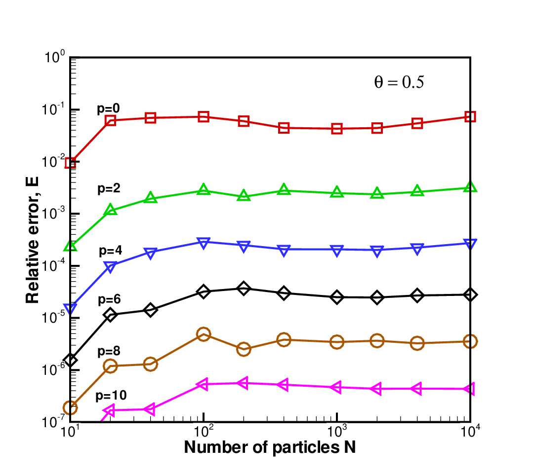
where is the exact potential on particle obtained by the direct summation method and is the potential obtained using treecode algorithm. The results are shown in Fig. 5. We can see that when , the error is almost independent of the system size The relative error decreases with the increase of order Although most counterions assemble near the macroion surface and the system is not uniform, when the error is already less than for and for .


Using Monte Carlo simulations, we also test the accuracy by investigating two physical properties of double layer structure: the radial distribution function (RDF), , of the counterions and the integrated charge distribution function (ICDF), , of the systems. In simulations, it is calculated using the average particle in a bin divided the volume of the bin and normalized the sum of all bins. The RDF describes the normalized average density along the radial direction. And the ICDF is a function of , which represents the average charge with the sphere of radius . Clearly, we have and . To observe the accuracy of these two functions, we plot the simulation results of and in Fig. 6. We see both functions converge to the results of direct summation, starting from . Shown in the inset plots, the errors are substantially in the same order as due to the fluctuation of the MC sampling, demonstrating that the multipole expansion with provides enough accuracy for describing the physical properties of the studied system. It can be observed that both and exponentially decay near the charged interface, in agreement with the prediction from the strong-coupling theory [4]. In contrast, the decay rate predicted by the classical Poisson-Boltzmann theory is algebraic [4], and thus these simulation results demonstrate the the theory fails for strong-coupling charged systems [18, 23].


Finally, the CPU times of the MC algorithm are compared for different strategies of the electrostatic calculations, with different system size and expansion order . The results have been shown in Fig. 7. Since the number of MC steps is of , it is illustrated that the CPU times for those curves with treecode acceleration scale as while that of direct summation scales as . The case of , which is accurate enough to provide correct RDF and ICDF curves, has the break-even point about Using the treecode acceleration, we find much larger systems can be explored, and the simulation for a system of can be done in a few days using the new MC algorithm, which is around times faster than that of the direct summation.

5 conclusion
In this paper, we have developed an efficient generalization of the Barnes-Hut octree algorithm in Monte Carlo simulations of charged systems. In order to adapt the one-particle displacement of Metropolis Monte Carlo simulations, the algorithm introduces a local modification strategy of the tree structure, which leads to a low computational cost, namely, complexity in each Monte Carlo step. This allows us to simulate equilibrium properties of a system with more than ten thousand charged particles in personal computers.
Future goals of this project includes the parallelization of the treecode algorithm [33, 14], the incorporation into the multiscale reaction-field modeling of electrolytes and with image charges for colloidal suspensions [13, 36], and the exploration of properties of larger scaled systems.
The authors acknowledge the financial support from the Natural Science Foundation of China (Grants No.: 11101276 and 91130012). Z. X. acknowledges the support from the Alexander von Humboldt foundation for a research stay at the ICP, University of Stuttgart.
References
- \bahao
- [1] Allen, M. P., and Tildesley, D. J. Computer Simulations of Liquids. Oxford University Press, Oxford, 1987.
- [2] Appel, A. An efficient program for many-body simulations. SIAM J. Sci. Stat. Comput. 6 (1985), 85–103.
- [3] Barnes, J., and Hut, P. A hierarchical O(NlogN) force-calculation algorithm. Nature 324 (1986), 446–449.
- [4] Boroudjerdi, H., Kim, Y.-W., Naji, A., Netz, R. R., Schlagberger, X., and Serr, A. Statics and dynamics of strongly charged soft matter. Phys. Rep. 416 (2005), 129–199.
- [5] Cheng, H., Greengard, L., and Rokhlin, V. A fast adaptive multipole algorithm in three dimensions. J. Comput. Phys. 155 (1999), 468–498.
- [6] Darden, T. A., York, D. M., and Pedersen, L. G. Particle mesh Ewald: an Nlog(N) method for Ewald sums in large systems. J. Chem. Phys. 98 (1993), 10089–10092.
- [7] Deserno, M., Jim¨¦nez-¨¢ngeles, F., Holm, C., and Lozada-Cassou, M. Overcharging of dna in the presence of salt: Theory and simulation. J. Phys. Chem. B 105 (2001), 10983–10991.
- [8] Duan, Z. H., and Krasny, R. An Ewald summation based multipole method. J. Chem. Phys. 113 (2000), 3492–3495.
- [9] Duan, Z. H., and Krasny, R. An adaptive treecode for computing nonbonded potential energy in classical molecular systems. J. Comput. Chem. 22 (2001), 184–195.
- [10] Ewald, P. P. Die berechnung optischer und elektrostatischer gitterpotentiale. Ann. Phys. 369 (1921), 253–287.
- [11] French, R. H., Parsegian, V. A., Podgornik, R., Rajter, R. F., Jagota, A., Luo, J., Asthagiri, D., Chaudhury, M. K., Chiang, Y.-M., Granick, S., Kalinin, S., Kardar, M., Kjellander, R., Langreth, D. C., Lewis, J., Lustig, S., Wesolowski, D., Wettlaufer, J. S., Ching, W.-Y., Finnis, M., Houlihan, F., von Lilienfeld, O. A., van Oss, C. J., and Zemb, T. Long range interactions in nanoscale science. Rev. Mod. Phys. 82, 2 (2010), 1887–1944.
- [12] Frenkel, D., and Smit, B. Understanding molecular simulation: From algorithms to applications. Academic Press, New York, 2002.
- [13] Gan, Z., and Xu, Z. Multiple-image treatment of induced charges in Monte Carlo simulations of electrolytes near a spherical dielectric interface. Phys. Rev. E 84 (2011), 016705.
- [14] Geng, W., and Krasny, R. A treecode-accelerated boundary integral Poisson-Boltzmann solver for electrostatics of solvated biomolecules. J. Comput. Phys. 247 (2013), 62 – 78.
- [15] Gibbon, P., Speck, R., Karmakar, A., Arnold, L., Frings, W., Berberich, B., Reiter, D., and Masek, M. Progress in mesh-free plasma simulation with parallel tree codes. Plasma Science, IEEE Trans. on 38, 9 (2010), 2367–2376.
- [16] Greengard, L., and Rokhlin, V. A fast algorithm for particle simulations. J. Comput. Phys. 73 (1987), 325–348.
- [17] Greengard, L., and Rokhlin, V. A new version of the Fast Multipole Method for the Laplace equation in three dimensions. Acta Numerica 6 (1997), 229–269.
- [18] Grosberg, A. Y., Nguyen, T. T., and Shklovskii, B. I. Colloquium: The physics of charge inversion in chemical and biological systems. Rev. Mod. Phys. 74, 2 (Apr 2002), 329–345.
- [19] Hockney, R. W., and Eastwood, J. W. Computer simulation using particles. Taylor & Francis, 1988.
- [20] Kabadshow, I., and Dachsel, H. The error-controlled fast multipole method for open and periodic boundary conditions. Fast Methods for Long-Range Interactions in Complex Systems (2011), 85.
- [21] Kondrat, S., Georgi, N., Fedorov, M. V., and Kornyshev, A. A. A superionic state in nano-porous double-layer capacitors: insights from monte carlo simulations. Phys. Chem. Chem. Phys. 13 (2011), 11359–11366.
- [22] Lashuk, I., Chandramowlishwaran, A., Langston, H., Nguyen, T.-A., Sampath, R., Shringarpure, A., Vuduc, R., Ying, L., Zorin, D., and Biros, G. A massively parallel adaptive fast-multipole method on heterogeneous architectures. In High Performance Computing Networking, Storage and Analysis, Proceedings of the Conference on (2009), IEEE, pp. 1–12.
- [23] Lau, A. W. C., Lukatsky, D. B., Pincus, P., and Safran, S. A. Charge fluctuations and counterion condensation. Phys. Rev. E 65 (2002), 051502.
- [24] Li, P., Johnston, H., and Krasny, R. A Cartesian treecode for screened Coulomb interactions. J. Comput. Phys. 228 (2009), 3858–3868.
- [25] Lindsay, K., and Krasny, R. A particle method and adaptive treecode for vortex sheet motion in 3-D flow. J. Comput. Phys. 172 (2001), 879–907.
- [26] Linse, P. Simulation of charged colloids in solution. Adv. Polym. Sci. 185 (2005), 111–162.
- [27] Linse, P. Electrostatics in the presence of spherical dielectric discontinuities. J. Chem. Phys. 128 (2008), 214505.
- [28] Lyubartsev, A. P., Tang, J. X., Janmey, P. A., and Nordenskiöld, L. Electrostatically induced polyelectrolyte association of rodlike virus particles. Phys. Rev. Lett. 81 (1998), 5465–5468.
- [29] Manzanares, J., Murphy, W., Mafe, S., and Reiss, H. Numerical simulation of the nonequilibrium diffuse double layer in ion-exchange membranes. J. Phys. Chem. 97 (1993), 8524–8530.
- [30] Marzouk, Y. M., and Ghoniem, A. F. K-means clustering for optimal partitioning and dynamic load balancing of parallel hierarchical n-body simulations. J. Comp. Phys 207, 2 (2005), 493–528.
- [31] Metropolis, N., Rosenbluth, A. W., Rosenbluth, M. N., Teller, A. H., and Teller, E. Equation of state calculations by fast computing machines. J. Chem. Phys. 21 (1953), 1087.
- [32] Walker, D. A., Kowalczyk, B., de la Cruz, M. O., and Grzybowski, B. A. Electrostatics at the nanoscale. Nanoscale 3 (2011), 1316–1344.
- [33] Winkel, M., Speck, R., Hübner, H., Arnold, L., Krause, R., and Gibbon, P. A massively parallel, multi-disciplinary Barnes-Hut tree code for extreme-scale N-body simulations. Comput. Phys. Comm. 183 (2012), 880–889.
- [34] Xu, Z., and Cai, W. Fast analytical methods for macroscopic electrostatic models in biomolecular simulations. SIAM Rev. 53 (2011), 683–720.
- [35] Xu, Z., Cheng, X., and Yang, H. Treecode-based generalized Born method. J. Chem. Phys. 134 (2011), 064107.
- [36] Xu, Z., Liang, Y., and Xing, X. Mellin transform and image charge method for dielectric sphere in an electrolyte. SIAM J. Appl. Math. 73 (2013), 1396–1415.
- [37] Ying, L. A pedestrian introduction to fast multipole methods. Sci. China Math. 55 (2012), 1043–1051.
- [38] Ying, L., Biros, G., and Zorin, D. A kernel-independent adaptive fast multipole algorithm in two and three dimensions. J. Comput. Phys. 196 (2004), 591–626.