Astrophysical evidence for an extra dimension: phenomenology of a Kaluza Klein theory
Abstract
In this brief review we discuss the viability of a multidimensional geometrical theory with one compactified dimension. We discuss the case of a Kaluza Klein fifth dimensional theory, addressing the problem by an overview of the astrophysical phenomenology associated with this five dimensional theory. By comparing the predictions of our model with the features of the ordinary (four dimensional) Relativistic Astrophysics, we highlight some small but finite discrepancies, expectably detectible from the observations. We consider a class of static, vacuum solutions of free electromagnetic Kaluza Klein equations with three dimensional spherical symmetry. We explore the stability of the particle dynamics in these spacetimes, the construction of self gravitating stellar models and the emission spectrum generated by a charged particle falling on this stellar object. The matter dynamics in these geometries has been treated by a multipole approach adapted to the geometric theory with a compactified dimension.
keywords
Kaluza Klein theory; Dimensional compactification; Multipole expansion; Emission spectraPACS
PACS Nos.:04.50.Cd, 04.50.Gh.Received (Day Month Year)Revised (Day Month Year)
1 Introduction
Geometrical extra dimensional theories represent a good candidate for the GUT (Great Unification Theory) [1, 2], being often used in this framework in attempt to find a unified theory of the four fundamental forces through the geometrization of the other fields in addition to the gravity as described by General Relativity. These theories are also used in the development of theoretical models of the evolution of our Universe as emerging from the observation, in fact many cosmological theories have been derived, considering an implementation of an higher dimension number than the four of the original Einstein model ([3, 4, 5, 6, 7]).
On the other hand, the recent results of the LHC experiments are still the subject of many debates and theoretical studies aimed at finding a data interpretation in terms of a possible multidimensional scenario compatible with the recent constraints (see for example [8, 9, 10, 11, 12, 13, 14, 15]). Therefore there is a great interest in providing a theoretical model able to explain the role of the extra dimensions and their meaning in a world that looks like a four dimensional one, but up to now no experimental evidence could outline a signature of extra dimensions but they could simply fix restriction on the existing proposals (see for example [16, 17, 18, 19, 20, 21, 22, 23] and also [24, 25, 26, 27]).
This paper participates this discussion by presenting a series of recent developments on the possible observational scenarios provided as available from the Universe observation, that could lead to an analysis of the observed phenomena in terms of multi dimensional models.
In [28, 29, 30, 31, 32] it has been taken into account the dynamics of moving bodies subjected to strong gravitational fields, and it was studied the test particle motion in view of further developments in the exploration of the extended matter behavior in this context, as the accretion disks around compact objects in a possible multi dimensional Universe. Actually we explore the very distant objects by the observation of their emission spectra, and the jets in the electromagnetic band like x ray or gamma ray etc. Many of these phenomena, like GRBs for example, are today still being explored. The origin on these high energy phenomena is generally associated with the initial stages of the development in the birth of a black hole, but they are far from being well understood in a satisfactory model. We look at these phenomena as fruitful environment in which we can highlight the details attributable in general to theories alternative to the Einstein’s one. Finally as outlined in [31] the study of the multidimensional stellar structure could be an interesting investigation area of the main astrophysical implications of the higher dimensional gravity. This extra dimensional star model should provide a usually star as observed in the apparent four dimensional (4D) Universe, but with some peculiar characteristics due to the presence of an extra dimension which regulates the structure, the equilibrium configuration and possibly its evolutionary history towards its final stages, see also [33, 34, 35, 36].
However besides the problem of the experimental proof of the existence of a possible extra dimension there are several subtle issues related to these theories. Firstly it should be clearly explained why one does not perceive the presence of one or more extra dimension as provided by the theory. There are several viable proposals to this question, and the two main different elaborations of this problem consists on one hand in the assumption of a very large extra dimensional size and on the other hand the conjecture of a very small extra dimension, that is below the Planck scale[37, 38, 39], for example this is the case of the 5D Kaluza Klein (KK) models. This is accomplished in different ways, however, we refer in this paper to the compactification of the extra dimension. In general, the Kaluza Klein models provide the geometrization of the electromagnetic field coupled with the gravitational one. In this review we consider a free electromagnetic 5D KK model with a scalar field associated to the extra dimensional component of the metric which regulates its the size and dynamics. These theories are characterized by the gauge invariance (spacetime symmetry) implemented by the invariance for translations on the compactified fifth dimension, representing the internal U(1) gauge symmetry via an isometric group. Nevertheless, the test particle dynamics constitutes a significant shortcoming known as the charge to mass puzzle: because of the huge massive modes arising near the Planck scale, it is possible to recover the particle motion but at the cost of the charge to mass ratio not matching with any observed particle.
It was recently proposed a revision of the dynamics in KK theories with compactified dimensions that seems to solve this problem without affecting the correct representation of the reduced 4D physical Universe [42]: specifically it has been taken into account a definition of a 5D particle as a localized matter distribution in the ordinary 4D spacetime but as a delocalized one on the fifth dimension. This starting point leads to a different definition of mass which solves the charge to mass puzzle: the procedure of the dimensional reduction from the 5D to 4D dynamics is based on a Papapetrou multipole expansion of a 5D energy momentum tensor which is supposed to be picked along a 4D world tube. Here we take into account a family of solutions of the KK equations in vacuum, known as Generalized Schwarzschild spacetime (GSS)[28, 44, 45]. These metrics are generally interpreted as an extension of the Schwarzschild spacetime to a 5D scenario, because in appropriate limits on the family parameters on the slice (the 4D metric counterpart), the GSS tensor reduces to the Schwarzschild metric.
The particle motion has been addressed in [28] using an effective potential approach. The test particle dynamics, circularly orbiting around a compact object is studied as a 1D nonrelativistic motion, governed by an effective potential which encloses the gravitational field, the centrifugal force and the effects due to the size variation of the extra dimension. We review the morphology of the circular motion by fixing the last circular orbit radius and the last stable circular orbits radius of charged and neutral test particles. These studies show that even in this simple spacetime model, some small but finite deformations of the physics with respect to the prediction of the 4D model appear. It is finally interesting to note that a deformation was found in [30] in the emission spectrum generated by a charged particle falling in a GSS towards the surface of a stellar object. Therefore the extra dimensional phenomenology of an Astrophysical setting could be an valuable environment in which searching for the signature of an extra dimension presence. In fact, the additional extra dimensional produces a nontrivial departure from the dynamics in the corresponding 4D counterpart of the GSS. We believe that this modification from the results expected in the 4D model can be even more evident in the dynamics of the extended matter configurations, for example in accretion disk scenarios.
The aim of this review is to focus attention on the possibility to highlight finite and observable effects from the presence of an extra dimension, by using an astrophysical scenario. The basic idea is that the emitted radiation is produced in a region of the space, near the compact 5D star, where this dimension is not compactified on a Planckian scale and therefore it affects the phenomenology of the emitting source, but there features are detected at very large distance, where the space resembles an Euclidean (asymptotically flat) one endowed with an unobservable compactified dimension. In this sense, the astrophysical setting offers the most natural arena for investigating the phenomenology of extra dimensions: the elementary particles (photons or more in general cosmic rays) are detected in the ordinary four dimensional Minkowski spacetime, where no direct measurement of the additional dimensions could be physically allowed, but they bring together information of the multi dimensionality of the spacetime region where it was produced. The present analysis, putting together different results present in the literature and providing them with a precise link, defines the necessary algorithm to use this powerful investigation scenario. The fundamental steps can be summarized as follows: i) a satisfactory paradigm to interpret the four dimensional matter (particle) phenomenology in term of the geometrical structure of the extra space, ii) the multidimensional version of a compact astrophysical object (star or black hole); associated with an interior or vacuum solution of the spherically or axially symmetric problem; iii) the detailed calculation of the particle energy spectrum as predicted by the phenomenology nearby the surface (or horizon) of such generalized sources.
Limiting the attention to a pure 5D Kaluza Klein scenario, this review successes in achieving all these three steps and therefore it constitutes a valuable framework, following which more general investigation can start up.
This paper is structured as follows: In Sec. (2) we illustrate the main characteristics of the 5D KK model and we discuss the test particle motion in the KK theory according to the standard approach. In Sec. (3) the alternative scenario for the matter behavior in KK compactified theories is introduced by Papapetrou’s approach. We discuss the resulting formulation of the motion and the KK field equation. Generalized Schwarzschild spacetime (GSS) is introduced in Sec. (4). Test particle dynamics in this spacetime is explored in Sec. (5). Star models in the 5D KK theories are introduced in Sec. (6). The study of the spectral emission of charged particles radially infalling in a GSS spacetime is discussed in Sec. (7). Finally Sec. (8) closes this paper with the discussions and future perspectives.
2 Five dimensional Kaluza Klein model
In this paper we investigate the astrophysical systems in the scenario envisaged by the 5D KK models, and looking for evidence that the 4D Universe would emerge as a dimensional reduction of the KK spacetime. Therefore this KK hypothesis requires the process of the dimensional reduction be satisfactory addressed. The fundamental requirement to make unobservable the fifth dimension is the existence of a closed topology which allows to compactify the spacetime. The basic request to deal with a closed topology is the periodicity of the metric field on the fifth coordinate, which allows to expand the Einstein Hilbert action in Fourier series and so to develop the dynamics of the different harmonics. This approach is intrinsically different from the cylindricity condition, due to Kaluza, which prescribes the independence of the metric tensor by the fifth coordinate, directly within the field equations. However, if we truncate the Einstein Hilbert action to the zero order and, we impose the closure of the fifth coordinate in the field equations independent of , the two approaches formally overlap. In fact, the variation of the zero order Lagrangian, after the integration on the extra coordinate has been performed coincides without further restrictions with the Einstein equations.
Thus, the KK spacetime is a 5D manifold , direct product , between the ordinary 4D spacetime and the space like loop [46, 47]. The size on the fifth dimension is assumed to be below the present observational bound or we here refer to this assumption as the “Compactification hypothesis”, and the metrics components do not depend on the fifth coordinate (Cylindricity hypothesis): this hypothesis can be realized assuming we are working in an effective theory at the lowest order of the Fourier expansion along the fifth dimension [44].
Moreover it is assumed that the metric component is a scalar . In this way the evolution of size of the fifth dimension, is entirely controlled by the dynamics of a geometrized real scalar field. According to the KK dimensional reduction the 5D line element reads11 1 With latin capital letters we label the 5D indices, where they run in , Greek and latin indices run from 0 to 3, the spatial indexes in . We consider metric of signature. We adopt coordinates for the ordinary 4D spacetime while is the angle parameter for the fifth circular dimension. as follows:
| (1) |
represents the 4D vector potential and is the 4D metric tensor; is a dimensional constant such that , where stays for the 4D gravitational constant. In general the KK setup is characterized by the breaking of the 5D covariance and the 5D equivalence principle [47], even if the translations along the fifth dimension are allowed to realized the abelian gauge invariance of the electromagnetism implemented in the KK model as a coordinate transformation in .
2.1 Particle motion in Kaluza Klein theory: the standard approach
In the standard, namely “geodesic” approach, the matter dynamics in the KK theories is generally faced assuming the existence of a 5D point like test particle in . In [40, 41, 42] this assumption has been revisited and the validity of a model with a point like particle in a compactified dimension is criticized.
The geodesic approach relies on the assumption that the 5D particle motion is regulated by a 5D Klein Gordon dispersion relations , where is the 5 momentum and is a constant mass parameter associated to the particle, in particular the component is conserved and it defines the particle charge by the the 5D velocities and the 4D velocities are defined respectively as , , with and , , where the parameter reads , and ( states for the 4D (5D) line element. The dimensional reduction of the equation of motion (the 5D geodesic: ) is recovered, furthermore the cylindric condition provides a constant of motion in agreement with the existence of the Killing vector . The mass parameter is assumed to be constant. The dimensional reduction leads to the set
| (2) | |||||
| (3) |
where is the Faraday tensor. Hence, in the standard scenario a free 5D test particle becomes a 4D interacting particle, whose motion is described by Eqs. (2).
We note that in particular for (neutral test particle case) Eq. (2) becomes a geodesic one. Moreover, even in a free electromagnetic scenario, the charged particles (with ) do not follow in general a geodesic motion, being coupled with the extra dimensional scalar field by a function. There is in fact in Eq. (4) a force term determined by the electromagnetic field (no more geometrized in the 4D scenario reduced from the 5D KK model) and by the scalar field dynamics. Any variation of the fifth dimension size appears as a force on the particle motion in the 4D Universe. With a constant scale factor the last term on the right side in Eq. (2) vanishes. The coupling factors are functions of , in particular the electrodynamic (EM) coupling factors, in terms of the effective particle charge to mass ratio is
| (4) |
Noticeably the right side of Eq. (4) is in general no constant and it is always upper bounded. Even if one sets , that is within the assumption that the extra dimension has a constant size, it is which is unacceptable for every known elementary particle. This problem is related to the huge massive mode of the KK tower ([40, 41, 42]). The alternative dynamic model, discussed in the next section seems to solve in particular this problem.
3 Alternative scenario: the Papapetrou’s approach
3.1 Papapetrou approach to the particle dynamics in the Kaluza Klein model
In [40, 41, 42] a new proposal for the matter dynamics in the KK model is given, adopting a Papapetrou multipole expansion [48] within the compactification hypothesis: extending the cylindricity hypothesis to a generic 5D matter tensor it is assumed that the particle is described as a localized source in but still delocalized along the fifth dimension. This hypothesis relays on the idea that, since the fifth dimension is compactified to Planckian like scales, it makes no sense to handle with a classical fifth component of the particle velocity and therefore this leads to the treatment of the matter sources through the energy momentum description. Such a point of view leads to adopt a Papapetrou scheme [48] to fix the dimensionally reduced equation of motion for fields and the matter. Performing the dimensional reduction either for the metric fields and the matter it is provided a consistent approach that removes the problem of huge massive modes, hence a consistent set of equations is wrote[32].
First a 5D energy momentum tensor is associated to the generic 5D matter distribution governed by the conservation law and not depending on the fifth coordinate, thus (here is the covariant derivative compatible with the 5D metric). Performing a multipole expansion of , centered on a trajectory , the lowest order of the procedure gives the equation of motion for a test particle:
| (5) |
The coupling factors are the charge , coming from the current vector and the scalar charge as follows,
| (6) | |||||
| (7) | |||||
| (8) |
these relations provide also the definitions for coupling factor , , and the according definitions for the effective test particle tensor and reads , where is the determinant of the 4D metric[30, 28]. The Eq. (5) describes the motion of a point like particle of mass in the 4D spacetime, coupled to the electromagnetic field through the charge and to the scalar field by the new quantity . The continuity equation , derived within the procedure itself, implies that charge is conserved. The parameter correctly represents the mass of the particle, which turns out to be localized just in the ordinary 4D space, as it is envisaged by the presence of a 4D Dirac delta function in the above definitions. It can be proved that the KK tower of massive modes is suppressed, and the ratio is no more upper bounded. Indeed, it can be proved that the motion of the particle is correctly governed by a dispersion relation of the form where here and in the following the dimensional index is dropped. Nevertheless, in general as a consequence of the coupling to the scalar field, the mass is now variable and it is precisely related to the variation of the scalar field and the new coupling (which has a pure extra dimensional origin) along the path. An interesting scenario concerning to be investigated is : by this way Eq. (5) admits an easy integration, providing a power law dependence of the mass on the scalar field and, more important, restoring the particle free falling universality when a vanishing electromagnetic field is considered, while the requirement , implies that the mass is constant.
3.2 Kaluza Klein field equations
The revision of the consequences of the dimensional compactification in the KK spacetimes has finally led to the reformulation of the field equations in the matter in this revisited KK context. The full system of the 5D Einstein equation in presence of the 5D matter described by a 5D matter tensor is:
| (9) |
where the 5D Bianchi identity holds, while from the cylindricity hypothesis concerning the matter field it is where is the 5D Newton constant, , and , where the coordinate length of the extra dimension . The components , , are a 4D tensor, a 4D vector and a scalar respectively. Introducing the quantities , , and , we have:
| (10) |
that introduces a conserved current , related to the U(1) gauge symmetry and coupled to the tensor , together with the conservation equation for
| (11) |
coupled to the field and by the matter terms and and representing the energy momentum density of the ordinary 4D matter.
In the limit we recover the conservation law for an electrodynamic system, and setting it is . Taking now into account these definitions, the reduction of Eq. (9) leads to the set
| (12) | |||||
| (13) |
for the Einstein and KK field, where
| (14) |
the KK Maxwell equation is now
| (15) |
In such a scenario the function is still undetermined and it should be fixed for a given background, while the reduced field equations correctly describe an Einstein Maxwell system and the full KK dynamics in presence of the matter source terms. The model function plays a similar role to the model parameter in the equations for the test particle dynamics. With respect to the pure Einstein Maxwell system there are now two additional scalar fields: the usual KK scalar field, , plus a scalar source term, .
4 Generalized Schwarzschild spacetime
In this section we introduce a special family of metrics, solutions of the electromagnetic free 5D vacuum KK equations ([49, 50, 51]). This metric family has many remarkable properties: firstly its 4D counterpart is spherical symmetric (4D spherical symmetry) and it is time independent: the ordinary 4D spacetime of the direct product is spherically symmetric; in other words the sections , and of are (spherical surfaces in the ordinary 3D space). In addition, for suitable limits on the family parameters these solutions can be reduced in their 4D counterpart to the Schwarzschild metric. For this reason this set of solutions is also known in the literature as Generalized Schwarzschild spacetime (GSS). This is a particularly interesting and versatile case to study because of its symmetric properties, and the amenability to a known 4D spacetime scenario widely studied in the astrophysics of the 4D Universe,

The one parameter family of metrics is
| (16) |
in the 4D spherical polar coordinate22 2 Consider , , , where , where , with is a constant. Each values of the parameter sets a specific metric of the family, the parameter is in fact constrained by . For a review about the constraints on the parameter see [44] and [32]. The GSSs are asymptotically flat and, for each finite value of , GSS has a naked singularity situated in , that resolves in a black hole only in the Schwarzschild limit for . The Schwarzschild limit is recovered on the spacetime section for .
Moreover, as approaches , reduces to zero while explodes to infinity, therefore the length of the extra dimension increases as well as approaches , Fig. (1).
These solutions represent extended objects: the GSS naked singularity is surrounded by the induced scalar matter with a trace free energy momentum tensor.
The constant parameter is related to the mass of a central body which is supposed to act as source of the gravitational field. Noticeably, the Schwarzschild limit is obtained when , and in this limit is the Schwarzschild mass. In fact, the total mass of this configuration has been calculated with many different definitions (see for example [54]), we refer here to the gravitational mass , inside a 3D volume, as given by the Tolman-Whittaker formula: that can be written in isotropic coordinate as where is a constant related to the mass of the central body, (see [44] and references therein). This is, in the Schwarzschild limit, ; while, for each finite value of , it is at infinity and it goes to zero as closes the singularity and is the ordinary spatial 3D volume element.
Hence, for every finite values of , GSSs are naked singularities surrounded by the induced scalar matter, and only in the limit they are black holes with an horizon in and vacuum for .
But, despite of the naked singularity feature showed far from the Schwarzschild limit, GSSs are supposed to describe in principle the exterior spacetimes of any astrophysical sources characterized by the required symmetries, embedded in a cloud of a real scalar field. This consideration gave rise to the work in [31] where an internal solution of the 5D KK equations was found as model for a stellar object in the 4D Astrophysics. Here we consider GSS with as the (5D vacuum) spacetime, surrounding a compact object with a radius .
In the attempt to provide any possible constraints for the parameter many efforts have been made to simulate known astrophysical objects with a metric (16), ie it was attempted to identify a spacetime generated by the selected source (for example the solar system) with a certain family metric, associating the gravitational source to a specific , [44, 52, 53, 54]. However modelling the Sun by a GSS, requires a fine tuning of the characteristic parameter [55] and in any case the various works and estimates associated with this model show that extra dimensions should play a negligible role in the solar system dynamics. The tests elaborate in [28, 29, 30, 31, 32], and briefly discussed in the following sections, within the Papapetrou approach stay as a valid alternative to these studies.
5 Test particle dynamics in the Generalized Schwarzschild spacetimes: the Papapetrou analysis
In this section we illustrate the main results concerning the time like circular orbits in the GSS within the Papapetrou approach. Considering the 4D momentum the mass is a function of the radial coordinate , constant along the circular orbits (at fixed ). In the Schwarzschild limit, or asymptotically, where we have . It is always possible to build the constants of motion and defined as follows:
| (17) |
where and are metric Killing fields, thus and , functions of and , are interpreted as the energy at infinity of the particle and the total angular momentum, respectively.
Adopting the standard procedure we define an effective potential
| (18) |
describing the motion of a test particle of mass in a circular orbit around the source in terms of the 1D motion of a particle in an effective potential , [56]. This function of the position and the orbital angular momentum , takes into account the centrifugal effects, through the angular momentum, and the gravitational field through the explicit dependency on the metric components and . However, the dependence on the fifth dimension through the scalar field is enclosed by the mass factor that appears explicitly in Eq. (18), this term, as seen in Section (3.1), also depends on the particular KK model beyond the choice of the parameter .
The orbital angular momenta and the particle energy in terms of the orbital radius , can be obtained by solving the equation
| (19) |
Equation (19) can also be solved by the radius in terms of the orbital momentum . These radii will generally depend on the intrinsic properties of the source, and on the particular adopted Papapetrou model (), thus in this case it will be . As in the Schwarzschild case a set of particular orbits exist that determine the stability regions for circular orbits. Specifically, this is thelast circular orbit radius and the last stable circular orbit radius . These correspond to the maximum and minimum of the effective potential as a function of respectively. They are solution of Eq. (19) with for and for .
In general one can say that in the region there are no circular orbits, while circular orbits in are unstable, and finally all orbits with are stable. Clearly one can expect that these particular orbits and the regions of orbital existence and stability are deformed respect to the orbital regions in the 4D Schwarzschild case. Each GSS is in general characterized by a couple of different . However it is possible to show that turns to be a function of only. In [28] different scenarios for the test particle circular orbits were addressed considering the cases , constant and , where is a real number. In the next sections we will outline the main results of this research showing in particular the deformation of the orbital stability regions respect to the 4D Universe model.
5.1 The case
In the KK scenario defined by , all the charged and neutral test particles in the GSS follow a geodesic equation
| (20) |
in the ordinary 4D spacetime, where is a constant and no scalar field coupling term appears. The quantities with subscript , identify here and hereinafter the constant quantities determined by the initial conditions.
Studying the potential as function of the orbit radius , we find the particle energy and the angular momentum of the circular orbit [32]. We recover the last circular orbit radius and the last stable circular orbit radius
| (21) |
function of . It is and it reduces to the Schwarzschild limit for large [32, 42]. However, at the decreasing of , the last circular orbit radius approaches the point in particular for it is . On the other hand it is and for we have while in the Schwarzschild’s limit we have .
Thus, in this case the analysis of the circular orbits and their stability has provided a significant constraint on the possible GSS and the physics of the 4D reduced Universe by the KK Papapetrou procedure. Indeed, the orbital region where the circular motion is allowed and the orbital region in which these orbits are stable are in general larger then the analogous regions in Schwarzschild spacetime as much as the reduced solution deviates from its Schwarzschild limit. Fig. (2)-left shows the radii and as functions of and their asymptotic limits, the energy and the particle angular orbital momentum in the last stable circular orbit are plotted. It is its Schwarzschild’s limit for all values of , while () Schwarzschild’s limit value for , Fig. (2). However, as noted in [32] this fact should not be read as a direct consequence of a possible motion along the fifth dimension, since Eq. (20) does not depend on it, neither on . We interpret this fact as a feature related to the deformation of the Schwarzschild metric as long as is sufficiently small and this seems to be confirmed also by the fact that Eqs. (20) are the same that obtained from the geodesic approach with .
5.2 The case
In the model the particles follow the curves
| (22) |
Note that in this case the mass is in general a function of the adopted model through the selection of the parameter and indirectly function of the orbital radius through the scalar field , that regulates the size of the fifth dimension. However in the Schwarzschild limit it is and if we set it is .
From the effective potential we find:
| (23) |
It should be noted that the orbital radii in Eq. (23) do not explicitly depend on , Fig. (2)-center.

As for the model also in this case it is for each . Nevertheless we note that in the case , the energy and the momentum are considered as functions of only. The mass has been plotted in Fig. (3), as function of and .

5.3 The case
Finally we set , with . In this model the test particles will follow the curves
| (24) |
as for the case constant the mass is no more a constant, but here . The constant case is recovered with and . With the parameters , where and with . In [28] it was shown that for
and , notice that in this case the last stable circular orbit radius depends on the two free parameters, and . Moreover for , while for and , is possible. For we recover the same physical situations sketched in the case . Fig. (2)-right plots and as function of the planes of their asymptotical limits are also shown. We note that in general and the difference increases with .
6 Stars in five dimensional Kaluza Klein theory
In [41] a 5D interior solution of the KK equations was found that matches the GSS at some radius . The existence of such configuration allows to remove the naked singularity that characterizes the GSS. This solution has been interpreted as a 5D stellar model (say a KK star) with a perfect fluid coupled with scalar field such that a cloud of real scalar field surrounds the 4D object. This solution has been used as the source of the gravitational field in [30], in the analysis of the EM emission spectrum of a test particle radially infalling in this spacetime towards the surface of this stellar object.
The KK equations for the free electromagnetic case with are,
| (25) | |||||
| (26) |
with (4D) perfect fluid energy momentum tensor, , where the pressure and the density are related by the equation of state with constants. The metric has the form
| (27) |
where are functions of only. Some results of the numerical integration are shown in Fig. (4)-left: metric components and the matter density are plotted as function of the radial coordinate : fixing , some initial conditions are given as the central density and the scalar field at center with , both have been set as function of a free parameter , fixed a priori in order to match the GSS on the star boundary, see for details [31].

This stellar model represents a spherically symmetric and stationary star in the 4D Universe, whose matter can be described as a perfect fluid with a given polytropic equation of state. However, with respect to the correspondent solution of the Einstein equations that meet at the board the Schwarzschild metric, this KK star is surrounded by a claud of extended scalar matter. This is clearly a toy model, and yet it is still only a first attempt to study this kind of objects, and it should be studied with greater and deeper detail especially paying attention to the behavior of the ordinary matter by which it is supposed that the star is done. Another important issue concerns the equilibrium and the phases of the stellar evolution that eventually can lead to a collapse with the formation of a singularity. However we have assumed that the stellar surface is at some radius , it should be also noted that this radius can be, in general, very close to the Schwarzschild radius .
7 Electromagnetic radiation emitted by a radially falling particle
In [30] it has been provided the profile of the EM emission spectrum of a charged particle radially falling on a GSS toward a KK star: it was assumed that the source of the gravitational field was a 5D stellar object as discussed in Sec. (6). This assumption has led to some specific hypothesis on the boundary conditions for the differential equations describing the spectrum: having in mind that if the star model, solution of the 5D equations with a perfect fluid, “differs little” from the analogue 4D model, we assume the presence of a possible extra dimension went sought in the “small deformations” of the spectrum as expected in the EM emission from a charged particle infalling in the Schwarzschild spacetime. Here we concern on the simplest scenario where . Topic is discussed in more details in the cited works [29, 32]. We consider the charged particle dynamics in a region , with constant and we compare the dynamics in GSS with the dynamics in the Schwarzschild geometry.
In general, the motion of a radially falling particle is regulated by the component and component of the geodesic equation (20), with , see for example [44, 57]. We introduce here the concept of the velocity in the direction . while the locally measured radial velocity is where . The radius at which the radial velocity starts to decreases will be denoted [57] and in the Schwarzschild limit it is , otherwise we have . The velocities and are functions of and they tend to zero at (spatial) infinity. The radial velocity goes to zero in the limit , and the local measured velocity goes to for , see Figs. (5) and [42, 40, 29, 32].
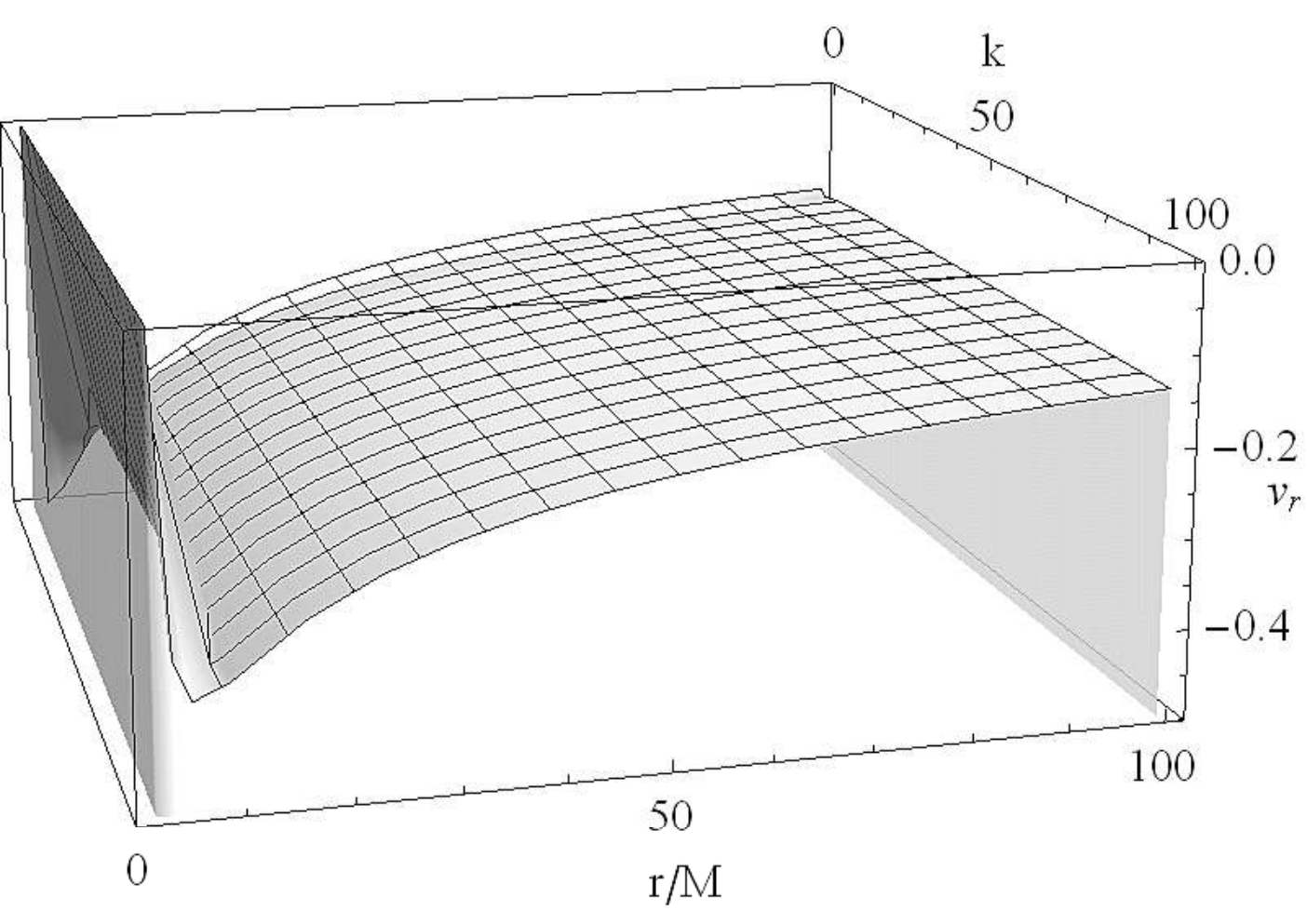

The charged test particle motion and the emitted EM radiation is considered as perturbations of the background metric, the EM radiation is regulated by
| (28) |
where is the Faraday tensor expanded in (4D) tensor harmonics , see [41]. In agreement with the Zerilli notation [58, 59, 60] denotes the radial (angle independent) part of the Faraday tensor, while the is the 4D current [41, 40], thus according with the Zerilli’s procedure, we find the following equation
| (29) |
and is the source term explicitly given in [30], this is a function of and , where is the (radial) particle velocity at spatial infinity and of the potential :
| (30) |
where
| (31) |
(see[58, 59, 60, 30] for the current use of the notation). In [30] the Sturm Liouville problem for the function was solved using the Green’s functions method. First the associated homogeneous () equation has been solved. We used the solutions of this equation to build the Green’s function of the problem. It was required that the outgoing radiation is purely oscillating at infinity. The energy spectra at (spatial) infinity was therefore given by
| (32) |
where and where is a function of only. Adopting a Runge Kutta method, we first integrated the homogeneous equation for a fixed value of to obtain an evaluation of the function with the required boundary condition. The numerical integration started at , that is a source boundary very close to the Schwarzschild limit . It is stopped at large values of as well as the integrals converge. We integrated Eq. (29) numerically for and for . The potential is plotted in Fig. (4)-center.
Once the values of the parameters are fixed, the integration has been performed for many fixed values of . It was so proved that the spectra profile, at large (say ) substantially coincides with the one emitted by a charged particle falling in the Schwarzschild background [61]. For a fixed , we note here that the homogeneous equation is a “Schrodinger-like” equation for the function with a potential . However, to fix the boundary conditions for a fixed is clearly important the analysis of the potential at infinity and at the starting point of integration. This function is plotted in Fig. (4)-center showing the dependence from and the parameter . Asymptotically, for large value of , the potential decreases to zero, it vanishes as approaches in the Schwarzschild limit. Far from this limit, ie for small values of on , the starting point of the integration, the potential is finite and very small (see details in [30]), this point in our model coincides with the boundary of the stellar object. We assume a regular condition on the stellar surface with respect to the radiation emitted by taking the potential to be zero a . The homogeneous equation is then solved imposing that the solution is ingoing at and a combination of “incident” and “transmitted” waves at spatial infinity. We have taken the star surface in is totally absorbent respect to the EM radiation that invests it, which therefore can be represented by the boundary condition on the surface with totally ingoing component. But within the context that we are analyzing the behavior of EM radiation which invests the gravitational source, has clearly an evolution determined by the gravitational field generated by the KK source. In Eq. (29) this information is encoded particularly in the potential, which is modulated by the distortion of the spacetime metric. In this regards, we note here some considerations concerning the . The emission spectrum, being in fact governed by the function , is determined by the boundary conditions that, according to this, are fixed. From Eq. (30) the potential depends on several variables, namely the radius , the multipole order , the source mass and the parameter , which precisely sets the background metric, but it does not directly depend on the scalar field and then from the extra dimension. The peculiar behavior of the potential at the Schwarzschild radius, differs greatly from the potential in the Schwarzschild spacetime diverging ar . This fact is not directly attributable to a possible influence of the extra dimension, but rather to the nature of the naked singularity located in , this speculation seems confirmed by the fact that the potential is stabilized (at a variation of ) in that point, being regularized to zero on the limit for the Schwarzschild metric parameters even in the full (not 4D reduced) 5D model, that is even when the scale of the extra dimension is a constant but . On the other hand, as discussed in Sec. (4), the scalar field that regulates the size of the fifth dimension diverges as one approaches the singularity. Other examples of similar studies which discuss the emission and electromagnetic propagation in the spacetime with naked singularity may be found in [62, 63, 64, 65, 66, 67, 68, 69, 70, 71, 72].
A spectra profile is plotted in Fig. (4)-left for and , see also [30]. A general feature of the emitted spectra for the Schwarzschild’s case is to grow up to a critical value (corresponding to a critical frequency for a fixed multipole) and then rapidly flow down to zero[61]. We found that for a fixed , the spectra profile coincides with that of the Schwarzschild’s case as well as is sufficiently large (). However there is an increase of the energy emitted rate per frequency , at fixed value of and fixed multipole . There are significant discrepancies with the Schwarzschild’s case for where, for low frequencies, a peak in the spectra profile appears also at large .
8 Discussions and future perspectives
A nontrivial question concerning any extra dimensional geometrical theory, arises on the non observation of the extra space in a Universe that is viewed according to the 4D model of the General Relativity. The compactified 5D Kaluza Klein theory provides a natural response to this problem assuming a closed extra space, with a volume much smaller then the minimal observed scale in the present day experiment of high energy physics, say . There is a great deal of attention in notice any discrepancies in the current observations with respect to the predictions of the standard theoretical setup, that could be possibly explained by an extra dimensional theory. Any experimental observation could provide then a strong constraint concerning the validity of the extra dimensional hypothesis. In particular one can search for new phenomena, unpredicted by the current models, but explained in a multi dimensional framework. One can search for the extra dimension evidences in the microscopic world [73, 74, 75, 76] or also in the astrophysical scenarios [77, 78, 79, 80, 81, 82, 83] In both cases, the validity of a multi dimensional theory is bounded for providing a theoretical model able to reproduce the compatibility of the extra dimension in a world that looks like a four dimensional one, requiring essentially the reproducibility of the reduced Universe and its physics in a suitable limit. In this respect a problem, in particular, plagues the 5D KK models concerning the particle charge to mass ratio as obtained from the geodesic motion in the standard approach: it is generally assumed the existence of a 5D particle generalizing its concept from the 4D Universe to a 5D world and assuming that the particle dynamics, not subjected to any forces in the compactified model, could be simply described with a 5D geodesic generalized from the equivalent 4D geodesic. Basically this approach states that the particle motion projected along the fifth dimension, when it is not subjected to forces in the KK spacetime, can be also a 5D geodesic. Recently, contesting the validity of the 5D geodesic assumption with respect to the projection on the compactified dimension, has emerged the need to address the issue of the test particle motion within the extra dimension with closed topology in a different way, which takes into account the quasi Plankian scale of this extra space. This problem was approached by a Papapetrou multipole expansion assuming a generic energy momentum tensor centered on the 4D trajectory. The resulted dynamic equations, are very promising and albeit able to describe correctly the 4D dynamics, they have proved to solve in particular the problem of the charge to mass ratio.
In this paper we adopt this multipole approach to the matter dynamics in the 5D spacetime of the KK model. We reformulated the test particle motion and the KK field equations finally arriving to a model of a 5D stellar configuration (KK star). We have presented a review of some astrophysical phenomenology that can lead, through the direct comparison between the observations and the model predictions, to test the multi dimension hypothesis viability. Following the works[28, 29, 30, 31, 32] we explored, by an effective potential approach to the motion, the dynamic stability around very compact objects; the stability regions and the energies of the moving bodies were found to be significantly different from those expected in the 4D model resulting from the Einstein theory. In [30] and in Sec. (7) of this review we have showed that the spectral analysis from the sources of the high energy Universe could in principle provide a test to constrain the multidimensional theories appearing in a departing of the EM emission spectra from that expected in general relativistic calculations (see also [16, 21, 25, 27, 61, 84, 85]). The construction of a stellar object in this extra dimensional scenario has consistently proved the existence of a source of the gravitational field, that looks, in the asymptotical limit of Minkowski spacetime as and ordinary star described by the Einstein equations. We have assumed particular spacetime symmetries such that this KK star can be conveniently viewed in comparison with the source of the Schwarzschild spacetime.
In conclusion the results, are convincing and promising under many respects. First, the revision of the dynamics in the compactified scenarios provided by the multipole expansion is capable to solve different problems of the standard approach to the KK models (in particular the charge to mass ratio puzzle for elementary particle). This reinterpretation started from a reasonable discussion on the laws of motion in the spacetime geometries with a Planckian scale dimension, investigating the consequences in the dynamics as seen in the macroscopic world.
The propose to search the effects of a possible extra dimension in the high energy Universe is convincing as confirmed by the results obtained also in the simple analysis of the test particle motion and the emission spectrum: the discrepancies highlighted between the predictions of these models and the general relativistic ones are small but may be detectable.
Acknowledgments
This work has been developed in the framework of the CGW Collaboration (www.cgwcollaboration.it). DP gratefully acknowledges financial support from the Angelo Della Riccia Foundation and wishes to thank the Blanceflor Boncompagni-Ludovisi, née Bildt 2012.
References
- [1] R. Bergamini and C. A. Orzalesi, Phys. Lett. B 135 (1984) 38.
- [2] A. Aranda, J. L. Diaz-Cruz and A. D. Rojas, Phys. Rev. D 80 (2009) 085027.
- [3] U. Gunther, P. Moniz and A. Zhuk, Astrophys. Space Sci. 283 (2003) 679.
- [4] P. Brax and C. van de Bruck, Class. Quant. Grav. 20 (2003) R201.
- [5] D. Langlois, Prog. Theor. Phys. Suppl. 148 (2003) 181.
- [6] E. Papantonopoulos, Lect. Notes Phys. 592 (2002) 458.
- [7] U. Günther, A. Starobinsky and A. Zhuk, Phys. Rev. D 69, 044003 (2004).
- [8] M. Arai, Gi-Chol Cho, K. Smolek, and K. Yoneyama Phys. Rev. D 87, 016010 (2013).
- [9] H. Sun, Y. -J. Zhou and H. Chen, Eur. Phys. J. 72 (2012) 2011.
- [10] D. Choudhury, A. Datta, D. K. Ghosh and K. Ghosh, JHEP 1204 (2012) 057.
- [11] J. de Blas, A. Delgado, B. Ostdiek and A. de la Puente, Phys. Rev. D 86 (2012) 015028.
- [12] Li Xiao-Zhou, Duan Peng-Fei, Ma Wen-Gan, Zhang Ren-You, and Guo Lei, Phys. Rev. D 86, 095008 (2012).
- [13] E. Gerwick, D. Litim and T. Plehn, Phys. Rev. D 83 (2011) 084048.
- [14] S. Arrenberg, L. Baudis, K. Kong, K. T. Matchev and J. Yoo, Phys. Rev. D 78 (2008) 056002.
- [15] X. Calmet, P. de Aquino and T. G. Rizzo, Phys. Lett. B 682 (2010) 446.
- [16] K. Matsuno and K. Umetsu, Phys. Rev. D 83 (2011) 064016.
- [17] T. G. Rizzo, AIP Conf. Proc. 530 (2000) 290.
- [18] M. Eingorn and A. Zhuk, Phys. Rev. D 83 (2011) 044005.
- [19] G. Moutsopoulos and P. Ritter, arXiv:1103.0152.
- [20] C. Stelea, K. Schleich and D. Witt, Phys. Rev. D 83 (2011) 084037.
- [21] J. Bonnevier, H. Melbeus, A. Merle and T. Ohlsson, arXiv:1104.1430.
- [22] H. Okawa, K. i. Nakao and M. Shibata, arXiv:1105.3331 [gr-qc].
- [23] S. Tomizawa and H. Ishihara, arXiv:1104.1468.
- [24] T. Moon, Y. S. Myung and E. J. Son, arXiv:1104.1908.
- [25] R. Becar and P. A. Gonzalez, arXiv:1104.0356.
- [26] Y. Yamada and H. a. Shinkai, Phys. Rev. D 83 (2011) 064006.
- [27] Q. Jiang, S.Yang, H. Li, Int. Journ. of Theoretical Physics, Vol. 45, No. 9, (2006).
- [28] V. Lacquaniti, G. Montani and D. Pugliese, Gen. Rel. Grav. 43, 4, (2011) 1103.
- [29] V. Lacquaniti, G. Montani, D. Pugliese, arXiv:0911.4168 [gr-qc].
- [30] D. Pugliese, G. Montani and V. Lacquaniti, Eur. Phys. J. C 71 (2011) 1747.
- [31] D. Pugliese and G. Montani, Eur. Phys. J. C 71 (2011) 1638.
- [32] V. Lacquaniti, G. Montani, D. Pugliese and R. Ruffini, arXiv:0912.2408 [gr-qc].
- [33] B. C. Paul, Int. J. Mod. Phys. D, Vol. 13, Issue 02, pp. 229-238 (2004).
- [34] S. Hannestad and G. G. Raffelt, Phys. Rev. D 67 (2003) 125008 [Erratum-ibid. D 69 (2004) 029901].
- [35] L. K. Patel and G. P. Singh, Grav. Cosmol. 7, 52 (2001).
- [36] P. K. Chattopadhyay, B. C. Paul, PRAMANA, journal physics, Vol. 74, No. 4, 2010 pp. 513-523.
- [37] T. Kaluza, On the Unity Problem of Physics, Sitzungseber. Press. Akad. Wiss. Phys. Math. ,1921.
- [38] O. Klein, Z.F.Physik, 37, 1926.
- [39] O. Klein, Nature, 118, 1926.
- [40] V. Lacquaniti and G. Montani, arXiv:0906.2231 [gr-qc].
- [41] V. Lacquaniti and G. Montani, Mod. Phys. Lett. A 24 (2009) 1565.
- [42] V. Lacquaniti and G. Montani, Int. J. Mod. Phys. D 18 (2009) 929.
- [43] F. Cianfrani, I. Milillo and G. Montani, Phys. Lett. A 366 (2007) 7.
- [44] J. M. Overduin and P. S. Wesson, Phys. Rept. 283 (1997) 303.
- [45] P. S. Wesson, “Space - time - matter: Modern Kaluza-Klein theory,” Singapore, Singapore: World Scientific (1999) 209 p.
- [46] D. Bailin and A. Love, Rept. Prog. Phys. 50 (1987) 1087.
- [47] Modern Kaluza-Klein Theories, edited by T. Applequist, A. Chodos, and P.G.O. Freund, Addison-Welsey, Menlo Park, 1987.
- [48] A. Papapetrou, Proc. Phys. Soc. 64, 57 (1951).
- [49] D. J. Gross and M. J. Perry, Nucl. Phys. B 226 (1983) 29.
- [50] R. D. Sorkin, Phys. Rev. Lett., 51, (1983) 87.
- [51] A. Davidson, D. A. Owen, Phys. Lett., 155B, (1985) 247.
- [52] P. Xu and Y. g. Ma, Phys. Lett. B 656 (2007) 165.
- [53] J. Ponce de Leon, Int. J. Mod. Phys. D 17 (2008) 237.
- [54] J. Ponce de Leon, Int. J. Mod. Phys. D 18 (2009) 251.
- [55] J. M. Overduin, Phys. Rev. D 62 (2000) 102001.
- [56] C. W. Misner, K. S. Thorne, & J. A. Wheeler, Gravitation, W. H. Freeman, 1973.
- [57] D. Kalligas, P. S. Wesson and C. W. F. Everitt, Astrophys. J. 439 (1994) 548.
- [58] F. J. Zerilli, Phys. Rev. D 2 (1970) 2141.
- [59] F. J. Zerilli, Phys. Rev. D 9 (1974) 860.
- [60] Les astres occlus-Les Houches, C. and B.S. De Witt (eds.), Gordon and Breach (New York, 1973).
- [61] V. Cardoso, J. P. S. Lemos and S. Yoshida, Phys. Rev. D 68 (2003) 084011.
- [62] G. Dotti and R. J. Gleiser, Class. Quant. Grav. 26 (2009) 215002.
- [63] Z. Kovacs and T. Harko, Phys. Rev. D 82 (2010) 124047.
- [64] R. Di Criscienzo, L. Vanzo and S. Zerbini, JHEP 1005 (2010) 092.
- [65] F. de Felice, Astronomy and Astrophysics, Vol. 34, p. 15 (1974).
- [66] R. Casadio, S. Fabi and B. Harms, Phys. Rev. D 70 (2004) 044026.
- [67] K. S. Virbhadra and C. R. Keeton, Phys. Rev. D 77 (2008) 124014.
- [68] K. S. Virbhadra and G. F. R. Ellis, Phys. Rev. D 65 (2002) 103004.
- [69] M. Patil, P.S. Joshi, D. Malafarina, Phys.Rev. D83 064007 (2011).
- [70] M. Patil, P. S. Joshi, Phys.Rev. D82 104049 (2010).
- [71] P. S. Joshi and D. Malafarina, Int. J. Mod. Phys. D 20 (2011) 2641.
- [72] M. Patil, P. S. Joshi, M. Kimura and K. -i. Nakao, Phys. Rev. D 86 (2012) 084023.
- [73] K. Kong, K. Matchev and G. Servant, arXiv:1001.4801 [hep-ph].
- [74] B. Bhattacherjee and K. Ghosh, with Phys. Rev. D 83 (2011) 034003.
- [75] A. Datta, K. Kong and K. T. Matchev, New J. Phys. 12 (2010) 075017.
- [76] R. Franceschini, G. F. Giudice, P. P. Giardino, P. Lodone and A. Strumia, arXiv:1101.4919 [hep-ph].
- [77] A. H. G. Peter, arXiv:1201.3942 [astro-ph.CO].
- [78] J. Einasto, arXiv:0901.0632 [astro-ph.CO].
- [79] M. Li, X. -D. Li, S. Wang and Y. Wang, Commun. Theor. Phys. 56 (2011) 525.
- [80] E. J. Copeland, M. Sami and S. Tsujikawa, Int. J. Mod. Phys. D 15 (2006) 1753.
- [81] J. Frieman, M. Turner and D. Huterer, Ann. Rev. Astron. Astrophys. 46 (2008) 385.
- [82] V. Sahni, Lect. Notes Phys. 653 (2004) 141.
- [83] M. Kamionkowski, arXiv:0706.2986 [astro-ph].
- [84] H. Liu and P. S. Wesson, J. Math. Phys. 42, 4963 (2001).
- [85] M. Cassé, J. Paul, G. Bertone, G. Sigl, Phys. Rev. Lett. 2004 Mar 19;92(11):111102.