Statistical Analysis of Metric Graph Reconstruction

Fabrizio Lecci lecci@cmu.edu Affiliation: Alessandro Rinaldo arinaldo@cmu.edu Affiliation: Larry Wasserman larry@cmu.edu Affiliation: Department of Statistics Affiliation: Carnegie Mellon University Affiliation: Pittsburgh, PA 15213, USA

Abstract

A metric graph is a 1-dimensional stratified metric space consisting of vertices and edges or loops glued together. Metric graphs can be naturally used to represent and model data that take the form of noisy filamentary structures, such as street maps, neurons, networks of rivers and galaxies. We consider the statistical problem of reconstructing the topology of a metric graph embedded in $\mathbb{R}^{D}$ from a random sample. We derive lower and upper bounds on the minimax risk for the noiseless case and tubular noise case. The upper bound is based on the reconstruction algorithm given in Aanjaneya et al. (2012).

^†^†heading: 1 2013 1-48 4/00 10/00 Fabrizio Lecci, Alessandro Rinaldo and Larry Wasserman^†^†shortheadings: Statistical Analysis of Metric Graph Reconstruction / Lecci, Rinaldo and Wasserman^†^†firstpage: 1

keywords

Metric Graph, Filament, Reconstruction, Manifold Learning, Minimax Estimation

1 Introduction

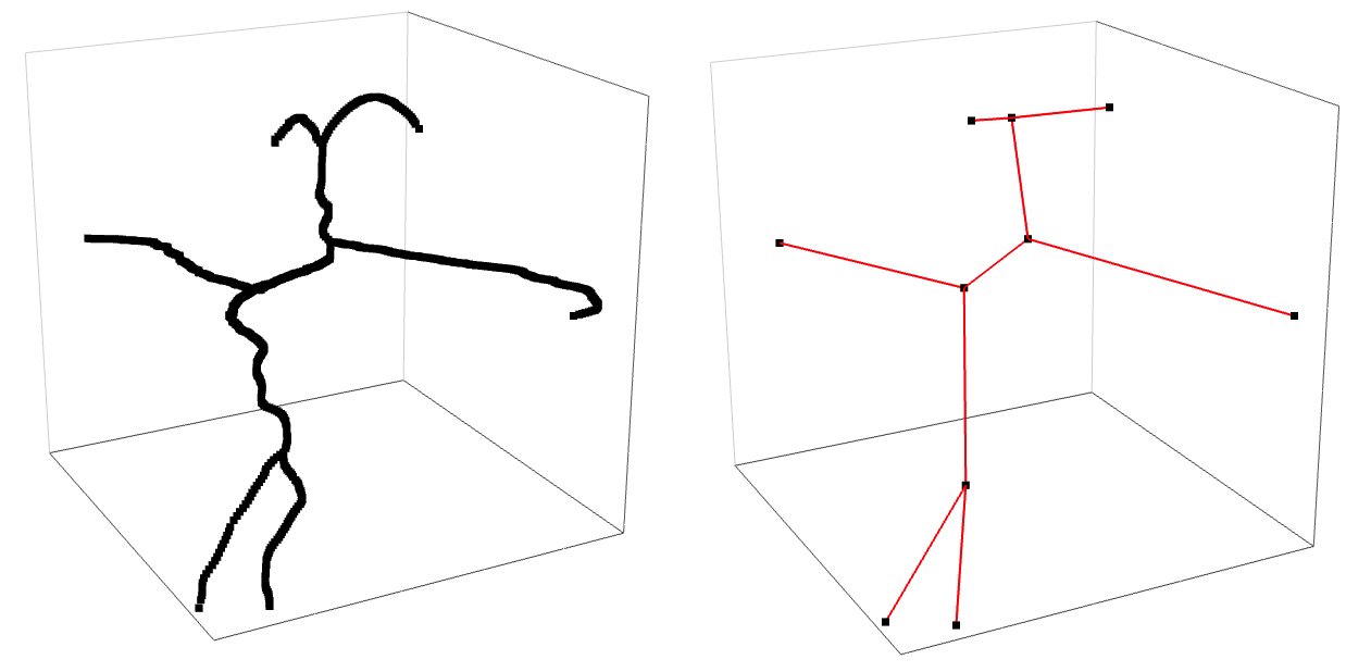
We are concerned with the problem of estimating the topology of filamentary data structure. Datasets consisting of points roughly aligned along intersecting or branching filamentary paths embedded in 2 or higher dimensional spaces have become an increasingly common type of data in a variety of scientific areas. For instance, road reconstruction based on GPS traces, localization of earthquakes faults, galaxy reconstruction are all instances of a more general problem of estimating basic topological features of an underlying filamentary structure. The recent paper by Aanjaneya et al. (2012), upon which our work is based, contains further applications, as well as numerous references. To provide a more concrete example, consider Figure 1. The left hand side displays raw data portraying a neuron from the hippocampus of a rat (Gulyás et al., 1999). The data were obtained from NeuroMorpho.Org (Ascoli et al., 2007). The right hand side of the figure shows the output of the metric graph reconstruction obtained using the algorithm analyzed in this paper, originally proposed by Aanjaneya et al. (2012). The reconstruction, which takes the form of a graph, captures perfectly all the topological features of the neuron, namely, the relationship between the edges and vertices, the number of branching points and the degree of each node.

Metric graphs provide the natural geometric framework for representing intersecting filamentary structures. A metric graph embedded in a $D$ -dimensional Euclidean space ( $D\geq 2$ ) is a 1-dimensional stratified metric space. It consists of a finite number of points (0-dimensional strata) and curves (1-dimensional strata) of finite length, where the boundary of each curve is given by a pair (of not-necessarily distinct) vertices (see the next section for a formal definition of a metric graph).

In this paper we study the problem of reconstructing the topology of metric graphs from possibly noisy data, from a statistical point of view. Specifically, we assume that we have a sample of points from a distribution supported on a metric graph or in a small neighborhood and we are interested in recovering the topology of the corresponding metric graph. To this end, we use the metric graph reconstruction algorithm given in Aanjaneya et al. (2012). Furthermore, in our theoretical analysis we characterize explicitly the minimal sample size required for perfect topological reconstruction as a direct function of parameters defining the shape of the metric graph, introduced in Section 2. This leads to an upper bound on the risk of topological reconstruction. Finally, we obtain a lower bound on the risk of topological reconstruction, which, in the noiseless case, almost matches the derived upper bound, indicating that the algorithm of Aanjaneya et al. (2012) behaves nearly optimally.

Outline. In Section 2 we formally define metric graphs, the statistical models we will consider and the assumptions we will use throughout. We will also describe several geometric quantities that are central to our analysis. Section 3 contains detailed analysis of the performance of algorithm of Aanjaneya et al. (2012) for metric graph reconstruction, under modified settings and assumptions. In Section 4 we derive lower and upper bounds for the minimax risk of metric graph reconstruction problem. In Section 5 we conclude with some final comments.

Related Work. The work most closely related to ours is Aanjaneya et al. (2012) which was, in fact, the motivation for our work. From the theoretical side, we replace the key assumption in Aanjaneya et al. (2012) of the sample being a $(\varepsilon,R)$ -approximation to the underlying metric graph, by the milder assumption of the sample being dense in a neigborhood of the metric graph. Approximation and reconstruction of metric graphs has also been considered in Chazal and Sun (2013) and Ge et al. (2011). Metric graph reconstruction is related to the problem of estimating stratified spaces (basically, intersecting manifolds). Stratified spaces have been studied by a number of authors such as Bendich et al. (2010); Bendich et al. (2012); Bendich (2008). A spectral method for estimating intersecting structures is given in Arias-Castro et al. (2011). There are a variety of algorithms for specific problems, for example, see Ahmed and Wenk (2012); Chen et al. (2010) for the reconstruction of road networks. Finally, Chernov and Kurlin (2013) derived an alternative algorithm that uses ideas from homology.

Refer to caption — Figure 1: Left: Neuron cr22e from the hippocampus of a rat; NeuroMorpho.Org (Ascoli et al., 2007). Right: A metric graph reconstruction of the neuron.

2 Background and Assumptions

The assumptions in Aanjaneya et al. (2012) lead to a reconstruction process that is aimed at capturing the intrinsic structure of the data and is somewhat oblivious to its extrinsic embedding. The authors assume that the sample comes with a metric that is close to the intrinsic metric of the underlying graph, by imposing a limit on the Gromov-Hausdorff distance between the two metrics. By considering data embedded in the Euclidean space and focusing on the topological aspect, we show that the notion of dense sample is sufficient to guarantee a correct reconstruction.

In this section we provide background on metric graph spaces and describe the assumptions and the geometric parameters that we will be using throughout.
Informally, a metric graph is a collection of vertices and edges glued together in some fashion. Here we state the formal definitions of path metric space and metric graph. For more details see Aanjaneya et al. (2012) and Kuchment (2004).

Definition 1.

A metric space $(G,d_{G})$ is a path metric space if the distance between any pair of points is equal to the infimum of the lengths of the continuous curves joining them. A metric graph is a path metric space $(G,d_{G})$ that is homeomorphic to a 1-dimensional stratified space. A vertex of $G$ is a 0-dimensional stratum of $G$ and an edge of $G$ is a 1-dimensional stratum of $G$ .

We will consider metric graphs embedded in $\mathbb{R}^{D}$ . Note that, if one ignores the metric structure, namely the length of edges and loops, the shape or topology of a metric graph $(G,d_{G})$ is encoded by a graph, whose vertices and edges correspond to vertices and edges of $G$ . Since we allow for two vertices to be connected by more than one edge we are actually dealing with pseudographs. We recall that an undirected pseudograph $(V,E)$ is a set of vertices $V$ , a multiset $E$ of unordered pairs of (not necessarily distinct) vertices. To a given pseudograph we can associate a function $f:E\rightarrow V\times V$ , which, when applied to an edge $e\in E$ , simply extracts the vertices to which $e$ is adjacent. Thus, if $e_{1},e_{2}\in E$ are such that $f(e_{1})=f(e_{2})$ , then $e_{1}$ and $e_{2}$ are parallel edges. Similarly, if $e\in E$ is such that $f(e)=\{v,v\}$ for some $v\in V$ , then $e$ is a loop. For each pair $(u,v)\in V\times V$ , let $\nu(u,v)=|f^{-1}(\{u,v\})|$ if $\{u,v\}\in E$ and $0$ otherwise. In particular, $\nu(u,v)$ is the number of edges between $u$ and $v$ (or loops if $u=v$ ).

We say that a metric graph reconstruction algorithm perfectly recovers the topology of $G$ if outputs a pseudograph isomorphic to the pseudograph representing the topology of $G$ .

We now define some key quantities regarding the structure of a metric graph. We start with the definition of reach. Let $M$ be a 1-dimensional manifold embedded in $\mathbb{R}^{D}$ . Let $T_{u}M$ denote the 1-dimensional tangent space to $M$ and let $T_{u}^{\perp}$ M be the $(D-1)$ -dimensional normal space.

Definition 2.

Define the fiber of size $a$ at $u\in M$ to be $L_{a}(u,M)=T_{u}^{\perp}M\bigcap B(u,a)$ , where $B(u,a)$ is the $D$ -dimensional ball of radius $a$ centered at $u$ . If $M$ has boundary $\{v_{1},v_{2}\}$ , the fiber of size $a$ at $v_{i}$ is defined as the limit of $L_{a}(u,M)$ , as $u$ approaches $v_{i}$ in $M\backslash\{v_{1},v_{2}\}$ . The reach of $M$ is the largest number $\tau$ such that the fibers $L_{\tau}(u,M)$ never intersect.

The reach sets a limit on the curvature of a manifold. A manifold with large reach does not come too close to be self-intersecting. For example the reach of an arc of a circle is equal to its radius. The quantity $1/\tau$ is called the condition number in Niyogi et al. (2008). For more details see also Federer (1959); Chazal and Lieutier (2006); Genovese et al. (2012a).
Each edge of a metric graph $(G,d_{G})$ can be seen as a 1-dimensional manifold with boundary. Let the local reach of metric graph $G$ be the minimum reach associated to an edge of $G$ .

When 2 edges intersect at a vertex $v$ they create an angle, where the angle between two intersecting curves is formally defined as follows. Suppose that $e_{1}$ and $e_{2}$ intersect at $x$ . Let $B(x,\epsilon)$ be the $D$ -dimensional ball of radius $\epsilon$ centered at $x$ . Let $\ell_{1}(\epsilon)$ be the line segment joining the two points $x$ and $\partial B(x,\epsilon)\bigcap e_{1}$ . Let $\ell_{2}(\epsilon)$ be the line segment joining the two points $x$ and $\partial B(x,\epsilon)\bigcap e_{2}$ . Let $\alpha_{\epsilon}(e_{1},e_{2})$ be the angle between $\ell_{1}(\epsilon)$ and $\ell_{2}(\epsilon)$ . The angle between $e_{1}$ and $e_{2}$ is $\alpha(e_{1},e_{2})=\lim_{\epsilon\to 0}\alpha_{\epsilon}(e_{1},e_{2})$ . We assume that, for each pair of intersecting edges $e_{1}$ and $e_{2}$ , the angle $\alpha(e_{1},e_{2})$ is well-defined.

To control points far away in the graph distance, but close in the embedding space, we define

A_{G}=\{(x,x^{\prime})\in G\times G:d_{G}(x,x^{\prime})\geq\min(b,\tau\alpha)\},

where $b$ is the shortest edge of $G$ , $\tau$ is the local condition number and $\alpha$ is the smallest angle formed by two edges of $G$ . We define the global reach as the infimum of the Euclidean distances among pairs of point in $A_{G}$ , that is $\xi=\inf_{A_{G}}\|x-x^{\prime}\|_{2}$ .

Let $(G,d_{G})$ be a metric graph and, for a constant $\sigma\geq 0$ , let $G_{\sigma}=\{y:\ \inf_{x\in G}||x-y||_{2}\leq\sigma\}$ be the $\sigma$ -tube around $G$ . If $\sigma=0$ , then, trivially, $G_{\sigma}=G$ . Notice that $G_{\sigma}$ is a set of dimension $D$ if $\sigma>0$ .

We will use the assumption that the sample $\mathbb{Y}$ is sufficiently dense in $G_{\sigma}$ with respect to the Euclidean metric, as formalized below.

Definition 3.

The sample $\mathbb{Y}=\{y_{1},\dots,y_{n}\}\subset G_{\sigma}\subset\mathbb{R}^{D}$ is $\frac{\delta}{2}$ -dense in $G_{\sigma}$ if for every $x\in G_{\sigma}$ , there exists a $y\in\mathbb{Y}$ such that $\|x-y\|_{2}<\frac{\delta}{2}$ .

The problem of metric graph reconstruction consists of reconstructing a metric graph $G$ given a dense sample $\{y_{1},\dots,y_{n}\}=\mathbb{Y}\subset G_{\sigma}$ endowed with a distance $d_{\mathbb{Y}}$ , which could be the $D$ -dimensional Euclidean distance or some more complicate notion of distance. If $\sigma=0$ we say that the sample $\mathbb{Y}$ is noiseless, while if $\sigma>0$ , we say that $\mathbb{Y}$ is a noisy sample.

Throughout our analysis we restrict the attention to metric graphs embedded in $\mathbb{R}^{D}$ that satisfy the following assumptions:

A1

The graphs have finite total length and are free of nodes of degree $2$ (though they may contain vertices of degree $1$ or $3$ and higher).
A2

Each edge is a smooth embedded sub-manifold of dimension 1, of length at least $b>0$ and with reach at least $\tau>0$ .
A3

Each pair of intersecting edges forms a well-defined angle of size at least $\alpha>0$ .
A4

The global reach is at least $\xi>0$ .

Assumptions A1 and A2 allow us to consider each edge of a metric graph as a single smooth curve. A3 and A4 are additional regularity conditions on the separation between different edges. Assumptions similar to A1-A4 are common in the literature. For different regularity conditions that allow for corners within an edge see, for example, Chazal et al. (2009) and Chen et al. (2010).

Let $\mathcal{G}$ be the set of metric graphs embedded in $\mathbb{R}^{D}$ that satisfy assumptions A1, A2, A3 and A4, involving the parameters $b$ , $\alpha$ , $\tau$ , $\xi$ . We consider two noise models:

Noiseless. We observe data $Y_{1},\dots,Y_{n}\sim P$ , where $P\in\mathcal{P}$ , a collection of probability distributions supported over metric graphs $(G,d_{G})$ in $\mathcal{G}$ having densities $p$ with respect to the length of $G$ bounded from below by a constant $a>0$ .

Tubular Noise. We observe data $Y_{1},\dots,Y_{n}\sim P_{G,\sigma}$ where $P_{G,\sigma}$ is uniform on the $\sigma$ -tube $G_{\sigma}$ . In this case we consider the collection $\mathcal{P}=\{P_{G,\sigma}:G\in\mathcal{G}\}$ .

We are interested in bounding the minimax risk

R_{n}=\inf_{\widehat{G}}\sup_{P\in\mathcal{P}}P^{n}\Big(\widehat{G}\not\simeq G\Big),

(1)

where the infimum is over all estimators $\widehat{G}$ of the topology of $(G,d_{G})$ , the supremum is over the class of distributions $\mathcal{P}$ for $\mathbb{Y}$ and $\widehat{G}\not\simeq G$ means that $\widehat{G}$ and $G$ are not isomorphic.
In Section 4 we will find lower and upper bounds for $R_{n}$ in the noiseless case and the tubular noise case.
We conclude this section by summarizing the many parameters and symbols involved in our analysis. See Table 1.

Symbol	Meaning
$(G,d_{G})$	metric graph
$\alpha$	smallest angle
$b$	shortest edge
$\tau$	local reach
$\xi$	global reach
$\mathcal{G}$	set of metric graphs embedded in $\mathbb{R}^{D}$ , satisfying A1-A4
$\mathcal{P}$	set of distributions on $G$ or $G_{\sigma}$
$G_{\sigma}$	$\sigma$ tube around $G$
$\mathbb{Y}$	sample, subset of $G_{\sigma}$
$\delta$	$\mathbb{Y}$ is a $\delta/2$ -dense sample

Table 1: Summary of the symbols used in our analysis.

3 Performance Analysis for the Algorithm of Aanjaneya et al. (2012)

In this section we study the performance of the metric graph reconstruction algorithm of Aanjaneya et al. (2012), under assumptions A1-A4 and with a choice of parameters adapted to our setting. In Section 4 we will use these results to derive bounds on the minimax rate for topology reconstruction. The metric graph reconstruction algorithm is presented in Algorithm 1.

Input: sample $\mathbb{Y},d_{\mathbb{Y}},r,p_{11}$ .
1: Labeling points as edge or vertex
2: for all $y\in\mathbb{Y}$ do
3: $S_{y}\leftarrow B(y,r+\delta)\backslash B(y,r)$
4: $\text{deg}_{r}(y)\leftarrow$ Number of connected components of Rips-Vietoris graph $\mathcal{R}_{\delta}(S_{y})$
5: if $\text{deg}_{r}(y)=2$ then
6: Label $y$ as a edge point
7: else
8: Label $y$ as a preliminary vertex point.
9: end if
10: end for.
11: Label all points within Euclidean distance $p_{11}$ from a preliminary vertex point as vertices.
12: Let $\mathbb{E}$ be the point of $\mathbb{Y}$ labeled as edge points.
13: Let $\mathbb{V}$ be the point of $\mathbb{Y}$ labeled as vertices.
14: Reconstructing the graph structure
15: Compute the connected components of the Rips-Vietoris graphs $\mathcal{R}_{\delta}(\mathbb{E})$ and $\mathcal{R}_{\delta}(\mathbb{V})$ .
16: Let the connected components of $\mathcal{R}_{\delta}(\mathbb{V})$ be the vertices of of the reconstructed graph $\widehat{G}$ .
17. Let there be an edge between vertices of $\widehat{G}$ if their corresponding connected components in $\mathcal{R}_{\delta}(\mathbb{V})$ contain points at distance less than $\delta$ from the same connected component of $\mathcal{R}_{\delta}(\mathbb{E})$ .
Output: $\widehat{G}$ .

Algorithm 1 Metric Graph Reconstruction Algorithm

The algorithm takes a (possibly noisy) sample $\mathbb{Y}$ from a metric graph $G$ and a distance $d_{\mathbb{Y}}$ defined on $\mathbb{Y}$ and returns a graph $\widehat{G}$ that approximates $G$ . The key idea is the following: a shell of radius $r$ is constructed around each point in the sample, which is labeled edge point if its shell contains 2 well separated clusters of sampled points and vertex point otherwise. Several steps of the algorithm require the construction of a Rips-Vietoris graph of parameter $\delta$ : $\mathcal{R}_{\delta}(S_{y})$ is a graph whose vertices are all the points of $S_{y}$ and there is an edge between two points if the Euclidean distance between them is not larger than $\delta$ . At Step 11 some of the edge points that are close to vertices are re-labeled as vertex points. This expansion guarantees a precise borderline between clusters of vertex points and clusters of edge points. At steps 15-17 each of these clusters is associated to a vertex or to an edge of the reconstructed graph $\widehat{G}$ . We will analyze the algorithm considering the Euclidean distance on the sample $\mathbb{Y}$ , that is, $d_{\mathbb{Y}}=\|\cdot\|_{2}$ . The inner radius of the shell at Step 3 and the width of the expansion at Step 11 are parameters the user has to specify.

Before finding how dense a sample has to be in orderer to guarantee a correct reconstruction of a metric graph, we show that it is sufficient to study a particular metric graph embedded in $\mathbb{R}^{2}$ , which represents the worst case. In other words, if the metric graph algorithm can reconstruct this particular planar graph, then it can reconstruct any other metric graph that satisfies A1-A4.

3.1 The worst case: a metric graph in $\mathbb{R}^{2}$

The worst case is the one for which it is hard to distinguish two edges that intersect at a vertex because they are too close in the embedding space.
Figure 2 (top left) shows an edge $e$ that intersects two edges $e_{1},e_{2}$ with reach $\tau$ , forming an angle $\alpha$ at vertex $x$ . For simplicity, we consider this metric graph embedded in $\mathbb{R}^{3}$ ( $D=3$ ). Therefore Figure 2 shows the projections of $e,e_{1}$ and $e_{2}$ on the (limit) plane formed by $e_{1}$ and $e_{2}$ , passing through $x$ .

Figure 2: Even in the worst case, edges

e_{1}

and

e_{2}

must lie outside of the torii constructed on the fibers

L_{\tau}(x,e_{1})

and

L_{\tau}(x,e_{2})

We focus on edge $e_{2}$ . The blue segment $\overline{AB}$ is the projection of $L_{\tau}(x,e_{2})$ , the fiber of size $\tau$ around $x$ . In $\mathbb{R}^{3}$ , $L_{\tau}(x,e_{2})$ is a circle of radius $\tau$ centered in $x$ . By definition, for any $y\in e_{2}$ , the fiber $L_{\tau}(y,e_{2})$ can not intersect the fiber $L_{\tau}(x,e_{2})$ , otherwise the assumption involving the reach would be violated. We represent this condition by taking a circle $C$ of radius $\tau$ centered at $B$ and rotating it around $x$ along the circumference of $L_{\tau}(x,e_{2})$ . This procedure forms a torus with an inner loop of radius 0. Edge $e_{2}$ must lie outside of this torus, so that its fibers do not intersect $L_{\tau}(x,e_{2})$ . See the top right plot of Figure 2.

The same reasoning applies to edge $e_{1}$ , which must lie outside of the torus constructed on $L_{\tau}(x,e_{1})$ . See the bottom left plot. The worst case is the one for which $e_{1}$ and $e_{2}$ are as close as possible: on the same plane and on the boundaries of the two tori. This case is represented in the bottom right plot of Figure 2. Note that $e_{1}$ and $e_{2}$ are simply arcs of circles of radius $\tau$ .

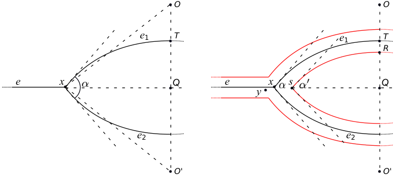
We will use basic trigonometric properties of the worst case. In Figure 3 (left), $O$ and $O^{\prime}$ are the centers of the circles associated to edges $e_{1}$ and $e_{2}$ . It is easy to see that angle $O\widehat{x}O^{\prime}$ has width $\pi-\alpha$ . It can be shown that

	$\displaystyle x\widehat{O}O^{\prime}$	$\displaystyle=\alpha/2,$		(2)
	$\displaystyle T\widehat{x}Q$	$\displaystyle=\alpha/4.$		(3)

Let $\mathbb{Y}$ be a noisy sample of $G$ . In other words $\mathbb{Y}$ is a subset of $G_{\sigma}$ , the tube of radius $\sigma\geq 0$ around the metric graph $G$ . See Figure 3 (right). Let $Q$ be the midpoint of segment $\overline{OO^{\prime}}$ and let $T$ be the intersection point of $\overline{OO^{\prime}}$ and edge $e_{1}$ . For $0\leq\sigma\leq\overline{QT}=\tau-\tau\cos(\alpha/2)$ , the smallest angle formed by the inner faces of the tube around the metric graph is

\alpha^{\prime}=\pi-\arccos\frac{2(\tau-\sigma)^{2}-4\tau^{2}\cos^{2}(\alpha/2)}{2(\tau-\sigma)^{2}},

(4)

where we applied the cosine law to the triangle $OsO^{\prime}$ and the fact that angle $O\widehat{s}O^{\prime}$ has width $\pi-\alpha^{\prime}$ . Note that if $\sigma=0$ then $\alpha^{\prime}=\alpha$ . As in (3), it can be shown that

R\widehat{s}Q=\alpha^{\prime}/4.

(5)

The few basic trigonometric equations described above will be used to determine under which conditions on $b,\alpha,\tau,\xi,\sigma$ the metric graph reconstruction algorithm can reconstruct the worst case.

3.2 Analysis of Algorithm 1 with Euclidean distance

In this section we analyze Algorithm 1. It is sufficient to study the worst case of figures 2 and 3 and extend the results to any metric graph in $\mathbb{R}^{D}$ . The Euclidean distance is used at every step of the algorithm, which requires the specification of $r$ , the inner radius of the shell, and $p_{11}$ , the parameter governing the expansion of Step 11. We set

r=\frac{\delta}{2}+\sigma+\tau\sin(\alpha/2)-(\tau-\sigma)\sin(\alpha^{\prime}/2)+\frac{\delta}{2\sin(\alpha^{\prime}/4)}

(6)

and

p_{11}=\frac{\delta}{2}+\tau\sin(\alpha/2)-(\tau-\sigma)\sin(\alpha^{\prime}/2)+\frac{r+\delta}{\sin(\alpha^{\prime}/2)}

(7)

This choice is justified in the proof of Proposition 4.
Define

		$\displaystyle f(b,\alpha,\tau,\xi,\sigma):=$
		$\displaystyle\frac{(\tau-\sigma)\sin\left(\frac{\min(b,\alpha\tau)-(\alpha-\alpha^{\prime})\tau}{2\tau}\right)-\left[\tau\sin(\alpha/2)-(\tau-\sigma)\sin(\alpha^{\prime}/2)\right]\left(1+\frac{2}{\sin(\alpha^{\prime}/2)}\right)-\frac{2\sigma}{\sin(\alpha^{\prime}/2)}}{1+3[\sin(\alpha^{\prime}/2)]^{-1}+[\sin(\alpha^{\prime}/2)\sin(\alpha^{\prime}/4)]^{-1}},$		(8)

where $\alpha^{\prime}$ is given in 4. Note that $f(b,\alpha,\tau,\xi,\sigma)$ is a decreasing function of $\sigma$ .

Proposition 4.

If $\mathbb{Y}$ is $\frac{\delta}{2}$ -dense in $G_{\sigma}$ and

0<r+\delta<\xi-2\sigma,

(9)

0<\delta<f(b,\alpha,\tau,\xi,\sigma),

(10)

then the graph $\widehat{G}$ provided by Algorithm 1 (input: $\mathbb{Y},\|\cdot\|_{2},r,p_{11}$ ) is isomorphic to $G$ .

Proof.

We will show that under conditions (9) and (10), Algorithm 1 can reconstruct the worst case described in section 3.1, formed by edges $e_{1}$ and $e_{2}$ of reach $\tau$ forming an angle of width $\alpha$ . This will automatically imply that the algorithm can reconstruct the topology of other vertices and edges in the $D$ -dimensional space.

Condition (9) guarantees that points of $G$ which are far apart in the metric graph distance $d_{G}$ , and close in the embedding space, do not interfere in the construction of the shells at Steps 3-4.

The rest of the proof involves condition (10). Since the sample is $\frac{\delta}{2}$ -dense in the tube, there is at least a point $y\in\mathbb{Y}$ inside the ball of radius $\frac{\delta}{2}$ centered at any vertex $x\in G$ . When using Algorithm 1 we want to be sure that $y$ is labeled as a vertex, that is, the number of connected components of the shell around $y$ is different than 2 (Steps 3-4). The worst case is depicted in Figure 4 (left), where $x$ is the vertex of minimum angle $\alpha$ , formed by two edges, $e_{1}$ and $e_{2}$ of reach $\tau$ . First, we show that for the the value of $r$ selected in (6), points close to an actual vertex are labeled as vertices at Steps 3-10 and points far from actual vertices are labeled as edges.

Figure 4: Left: edges

e_{1}

and

e_{2}

with minimum reach

\tau

forming the smallest angles

\alpha

at vertex

x

. Right: The distance

\|F-G\|_{2}

between the two connected components of the shell around an edge point

y^{\prime}

must be greater than

\delta

The inner faces of the tube of radius $\sigma$ around $e_{1}$ and $e_{2}$ form an angle of width $\alpha^{\prime}$ at vertex $s$ , as described in Section 3.1. Let $u$ and $v$ be the two points on the faces of the tube such that they are equidistant from $x$ and $\|u-v\|_{2}=\delta$ . Since at Step 4 we construct a $\delta$ -graph to determine the number of connected components of the shell $S_{y}$ and we want $y$ to be a vertex, we choose $r$ , the inner radius of the shell $S_{y}$ , so that if $u,v\in\mathbb{Y}$ then $r\geq\max\{d_{\mathbb{Y}}(y,u),d_{\mathbb{Y}}(y,v)\}$ . This guarantees that $\forall t_{1},t_{2}\in\mathbb{Y}$ with $t_{1}$ around edge $e_{1}$ , $t_{2}$ around edge $e_{2}$ such that $\{t_{1},t_{2}\}\subset S_{y}$ , we have $d_{\mathbb{Y}}(t_{1},t_{2})\geq\delta$ , that is $t_{1}$ and $t_{2}$ belong to different connected components of the shell around $y$ at Step 4.
The distance between $y$ and $u$ is bounded by $\|y-x\|_{2}+\|x-s\|_{2}+\|s-u\|_{2}$ , where, using (2),

\|x-s\|_{2}=\|x-Q\|_{2}-\|s-Q\|_{2}=\tau\sin(\alpha/2)-(\tau-\sigma)\sin(\alpha^{\prime}/2)

and using (5),

\|s-u\|_{2}\leq\frac{\delta}{2\sin(\alpha^{\prime}/4)}.

(11)

Therefore we require that $r$ , the inner radius of the shell of Step 4 satisfies

	$\displaystyle r$	$\displaystyle\geq\frac{\delta}{2}+\\|x-s\\|_{2}+\frac{\delta}{2\sin(\alpha^{\prime}/4)}$		(12)
		$\displaystyle\geq\\|y-x\\|_{2}+\\|x-s\\|_{2}+\\|s-u\\|_{2}.$

Another condition on $r$ arises when we label edge points far from actual vertices. See Figure 4 (right). If $y^{\prime}\in\mathbb{Y}$ , then it should be labeled as an edge point. That is, at Step 4, the Rips graph $\mathcal{R}_{\delta}(S_{y^{\prime}})$ on the shell $S_{y^{\prime}}$ should have 2 connected components. Therefore the distance $\|F-G\|_{2}$ between them must be greater than $\delta$ . We require that

r\geq 2\sigma+\delta/\sqrt{2}

(13)

which implies $\|F-G\|_{2}>\delta$ when $r$ is small enough, as implied by (10).
Note that the value $r=\frac{\delta}{2}+\sigma+\|x-s\|_{2}+\frac{\delta}{2\sin(\alpha^{\prime}/4)}$ satisfies both (12) and (13).

The outer radius of the shell at Steps 3-4 has length $r+\delta$ . This guarantees that when the shell around an edge point intersects the tube around $G$ there is at least a point $y\in\mathbb{Y}$ in each connected component of the shell, since $\mathbb{Y}$ is $\frac{\delta}{2}$ -dense in $G_{\sigma}$ .

In the last part of this proof we show that condition (10) is needed to guarantee that the sample is dense enough and the radius of the shells of Step 3 has the correct size, so that, even in the worst case, each vertex is associated to one set of sampled points at Steps 15-17 and these connected components are correctly linked by sets of sampled points labeled as edge points.
Let $z\in G_{\sigma}$ be the point around $e_{2}$ where the segment of length $r+\delta$ , orthogonal to the face of the tube around edge $e_{1}$ , intersects the face of the tube around edge $e_{2}$ . See Figure 5. If this segment does not exist we simply consider the segment of length $r+\delta$ from $s$ to a point $z$ on $e_{2}$ .

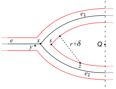
Suppose $z\in\mathbb{Y}$ . Among the points that might be labeled as vertices at Step 6 because of their closeness to vertex $x$ , $z$ is the furthest from $x$ , since the shell around $z$ is tangent to the tube around $e_{1}$ . At Step 11, in order to control the labelling of the points in the tube between $y$ and $z$ we would like to label all the points in $\{y^{\prime}\in\mathbb{Y}:\|y^{\prime}-y\|_{2}\leq\|y-z\|_{2}\}$ as vertices. To simplify the calculation we use the following bound

\displaystyle\|y-z\|_{2}

\displaystyle\leq\|y-x\|_{2}+\|x-s\|_{2}+\|s-z\|_{2},

where, using (5),

\|s-z\|_{2}\leq\frac{r+\delta}{\sin(\alpha^{\prime}/2)}.

(14)

This justifies the choice of $\displaystyle p_{11}=\frac{\delta}{2}+\|x-s\|_{2}+\frac{r+\delta}{\sin(\alpha^{\prime}/2)}\geq\|y-z\|_{2}$ . Thus, at Step 11 we label all the points in $\{y^{\prime}\in\mathbb{Y}:\|y^{\prime}-y\|_{2}\leq p_{11}\text{ and }y\text{ is labeled as vertex at Step 6 }\}$ as vertices. If $z$ is actually labeled as a vertex at Step 6, then through the expansion of Step 11, all the points at distance not greater than $p_{11}$ from $z$ are labeled as vertices.
Finally we determine under which conditions there is at least a point in the tube around $e_{2}$ labeled as an edge point after Step 11. Consider the worst case in which $e_{1}$ and $e_{2}$ are forming an angle of size $\alpha$ at both their extremes $x$ and $x^{\prime}$ . See Figure 6.

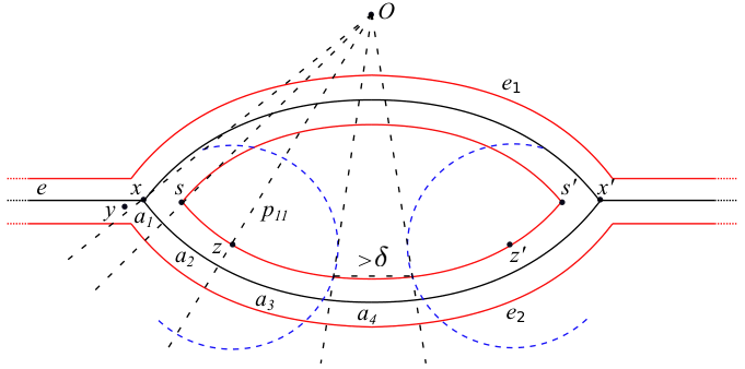
All the points $y^{\prime}\in\mathbb{Y}$ such that $\|y^{\prime}-z\|_{2}\leq p_{11}$ or $\|y^{\prime}-z^{\prime}\|_{2}\leq p_{11}$ might be labeled as vertices. When we construct $\mathcal{R}(\mathbb{E})_{\delta}$ and $\mathcal{R}(\mathbb{V})_{\delta}$ at Step 15 the two sets of vertices around $x$ and $x^{\prime}$ must be disconnected and there must be at least an edge point between them. A sufficient condition is that the length of edge $e_{2}$ is greater than $2(a_{1}+a_{2}+a_{3})+a_{4}$ , where

•

$a_{1}$ is the length of the arc of $e_{2}$ formed by the projections of lines $\overline{Ox}$ and $\overline{Os}$ on $e_{2}$ ,
•

$a_{2}$ is the length of the arc of $e_{2}$ formed by the projection of the chord of length $\|s-z\|_{2}$ ,
•

$a_{3}$ is the length of the arc of $e_{2}$ formed by the projection of the chord of length $p_{11}$ ,
•

$a_{4}$ is the length of the arc of $e_{2}$ formed by the projection of the chord of length $\delta$ .

Note that, in Figure 6, $e_{2}=2\tau\arcsin\left(\frac{\|x-x^{\prime}\|_{2}}{2\tau}\right)=\alpha\tau$ but in general it might be shorter, so that $e_{1}$ and $e_{2}$ might not intersect in $x^{\prime}$ . However, by assumptions A2, $e_{2}$ must be longer than $b$ . Thus we require

\min(b,\alpha\tau)>2(a_{1}+a_{2}+a_{3})+a_{4}.

(15)

By simple properties involving arcs and chords we have

	$\displaystyle a_{1}$	$\displaystyle=\left(\frac{\alpha-\alpha^{\prime}}{2}\right)\tau,\hskip 56.9055pta_{2}=2\tau\arcsin\left(\frac{\\|s-z\\|_{2}}{2(\tau-\sigma)}\right),$
	$\displaystyle a_{3}$	$\displaystyle=2\tau\arcsin\left(\frac{p_{11}}{2(\tau-\sigma)}\right),\quad a_{4}=2\tau\arcsin\left(\frac{\delta}{2(\tau-\sigma)}\right).$

Since the arcsin is superadditive in $[0,1]$ we require the stronger condition

\min(b,\alpha\tau)-(\alpha-\alpha^{\prime})\tau>2\tau\arcsin\left(\frac{2\|s-z\|_{2}+2p_{11}+\delta}{2(\tau-\sigma)}\right),

which holds if

\sin\left(\frac{\min(b,\alpha\tau)-(\alpha-\alpha^{\prime})\tau}{2\tau}\right)>\frac{2\frac{r+\delta}{\sin(\alpha^{\prime}/2)}+2p_{11}+\delta}{2(\tau-\sigma)}.

The last condition is equivalent to (10). If this condition is satisfied then the graph is correctly reconstructed at Steps 15-17: every connected component of $\mathcal{R}_{\delta}(\mathbb{V})$ corresponds to a vertex of $G$ and every connected component of $\mathcal{R}_{\delta}(\mathbb{E})$ corresponds to an edge of $G$ . ∎

Example 5.

A Neuron in Three-Dimensions. We return to the neuron example and we try to apply Propositions 4 to the 3D data of Figure 1, namely the neuron cr22e from the hippocampus of a rat (Gulyás et al., 1999). The data were obtained from NeuroMorpho.Org (Ascoli et al., 2007). The total length of the graph is $1750.86\mu m$ . We assume the smallest edge has length $100\mu m$ , the smallest angle $\pi/3$ , the local reach $30\mu m$ and $\xi=50\mu m$ . The conditions of Proposition 4 are satisfied for $\delta=2.00\mu m$ . Algorithm 1 reconstructs the topology of the metric graph starting from a $\delta/2$ -dense sample. Figure 1b shows the reconstructed graph.

4 Minimax Analysis

In this section we derive lower and upper bound for the minimax risk

R_{n}=\inf_{\widehat{G}}\sup_{P\in\mathcal{P}}P^{n}\Big(\widehat{G}\not\simeq G\Big),

(16)

where, as described in Section 2, the infimum is over all estimators $\widehat{G}$ of the metric graph $G$ , the supremum is over the class of distributions $\mathcal{P}$ for $\mathbb{Y}$ and $\widehat{G}\not\simeq G$ means that $\widehat{G}$ and $G$ are not isomorphic.

4.1 Lower Bounds

To derive a lower bound on the minimax risk, we make repeated use of Le Cam’s lemma. See, e.g., Yu (1997) and Chapter 2 of Tsybakov (2008). Recall that the total variation distance between two measures $P$ and $Q$ on the same probability space is defined by TV $(P,Q)=\sup_{A}|P(A)-Q(A)|$ where the supremum is over all measurable sets. It can be shown that TV $(P,Q)=P(H)-Q(H)$ , where $H=\{y:p(y)\geq q(y)\}$ and $p$ and $q$ are the densities of $P$ and $Q$ with respect to any measure that dominates both $P$ and $Q$ .

Lemma 6 (Le Cam).

Let $\mathcal{Q}$ be a set of distributions. Let $\theta(Q)$ take values in a metric space with metric $\rho$ . Let $Q_{1},Q_{2}\in\mathcal{Q}$ be any pair of distributions in $\mathcal{Q}$ . Let $Y_{1},\dots,Y_{n}$ be drawn iid from some $Q\in\mathcal{Q}$ and denote the corresponding product measure by $Q^{n}$ . Then

\inf_{\widehat{\theta}}\sup_{Q\in\mathcal{Q}}\mathbb{E}_{Q^{n}}\left[\rho(\widehat{\theta},\theta(Q))\right]\geq\frac{1}{8}\rho(\theta(Q_{1}),\theta(Q_{2}))(1-\text{TV}(Q_{1},Q_{2}))^{2n}

(17)

where the infimum is over all the estimators of $\theta(Q)$ .

Below we apply Le Cam’s lemma using several pairs of distributions. Any pair $Q_{1},Q_{2}$ is associated with a pair of metric graphs $G^{\prime},G^{\prime\prime}\in\mathcal{G}$ . We take $\theta(Q_{1})$ and $\theta(Q_{2})$ to be the classes of graphs that are isomorphic to $G^{\prime}$ and $G^{\prime\prime}$ . We set $\rho(\theta(Q_{1}),\theta(Q_{2}))=0$ if $G^{\prime}$ and $G^{\prime\prime}$ are isomorphic and $\rho(\theta(Q_{1}),\theta(Q_{2}))=1$ otherwise. Figure 7 shows several pairs of metric graphs that are used to derive lower bounds in the noiseless case and in the tubular noise case. In the noiseless case we ignore the $\sigma$ -tubes around the metric graphs.

Theorem 7.

In the noiseless case ( $\sigma=0$ ), for $b\leq b_{0}(a)$ , $\alpha\leq\alpha_{0}(a)$ , $\xi\leq\xi_{0}(a)$ , $\tau\leq\tau_{0}(a)$ , where $b_{0}(a),\alpha_{0}(a),\xi_{0}(a)$ and $\tau_{0}(a)$ are constants which depend on $a$ , a lower bound on the minimax risk for metric graph reconstruction is

R_{n}\geq\exp\Bigl(-2a\min\{b,2\sin(\alpha/2),\xi,2\pi\tau\}n\Bigr).

(18)

Proof.

We consider the 4 parameters separately. See Figure 7, ignoring the red lines representing the tubular noise that is not considered in this theorem.

Shortest edge $b$ . Consider the metric graph $G_{1}$ consisting of a single edge of length 1+ $b$ and metric graph $G_{2}$ with an edge of length 1 and an orthogonal edge of length $b$ glued in the middle. The density on $G_{1}$ is constructed in the following way: on the set $G_{1}\backslash G_{2}$ of length $b$ we set $p_{1}(x)=a$ and the rest of the mass is evenly distributed over the remaining portion of $G_{1}$ . Similarly, for $G_{2}$ we set $p_{2}(x)=a$ on $G_{2}\backslash G_{1}$ , which correspond to the orthogonal edge of length $b$ . We evenly spread the remaining mass. The two densities differ only on the sets $G_{1}\backslash G_{2}$ and $G_{2}\backslash G_{1}$ . Therefore $\text{TV}(p_{1},p_{2})\leq ab$ and, by Le Cam’s lemma, $R_{n}\geq\frac{1}{8}(1-ab)^{2n}\geq\frac{1}{8}\text{e}^{-2abn}$ for all $b\leq b_{0}(a)$ , where $b_{0}(a)$ is a constant depending on $a$ .

Smallest angle $\alpha$ . Now consider the metric graphs $G_{3}$ and $G_{4}$ . $G_{3}$ consists of two edges of length 2 forming an angle $\alpha$ and a third edge of length $1+2\sin(\alpha/2)$ glued to the first two. $G_{4}$ is similar: an edge of length $2\sin(\alpha/2)$ is added to complete the triangle, while the edge on the left has length 1. As in the previous case we set $p_{3}(x)=a$ on $G_{3}\backslash G_{4}$ , $p_{4}(x)=a$ on $G_{4}\backslash G_{3}$ and spread evenly the rest of the mass. The total variation distance is $\text{TV}(p_{3},p_{4})\leq 2a\sin\left(\frac{\alpha}{2}\right)$ and, by Le Cam’s lemma, $R_{n}\geq\frac{1}{8}(1-2a\sin\left(\alpha/2\right))^{2n}\geq\frac{1}{8}\text{e}^{-4a\sin\left(\alpha/2\right)n}$ for all $\alpha\leq\alpha_{0}(a)$ , where $\alpha_{0}(a)$ is a constant depending on $a$ .

Global reach $\xi$ . We defined the global reach as the shortest euclidean distance between two points that are far apart in the graph distance. Figure 7 shows metric graph $G_{5}$ formed by a single edge of length 1 and metric graph $G_{6}$ consisting of two edges of length $0.5$ , $\xi$ apart from each other. Again, we set $p_{5}(x)=a$ on $G_{5}\backslash G_{6}$ , $p_{6}(x)=a$ on $G_{6}\backslash G_{5}$ and evenly spread the rest. We obtain $\text{TV}(p_{5},p_{6})\leq a\xi$ and, by Le Cam’s lemma, $R_{n}\geq\frac{1}{8}(1-a\xi)^{2n}\geq\frac{1}{8}\text{e}^{-2a\xi n}$ for all $\xi\leq\xi_{0}(a)$ , where $\xi_{0}(a)$ is a constant depending on $a$ .

Local reach $\tau$ . The local reach $\tau$ is the smallest reach of the edges forming the metric graph. Consider metric graphs $G_{7}$ and $G_{8}$ . $G_{7}$ consists of a loop of radius $\tau$ attached to an edge of length 1 and metric graph $G_{8}$ is a single edge of length $1+2\pi\tau$ . As in the previous cases $p_{7}(x)=a$ on $G_{7}\backslash G_{8}$ and $p_{8}(x)=a$ on $G_{8}\backslash G_{7}$ . It follows that $\text{TV}(p_{7},p_{8})\leq 2a\pi\tau$ and, by Le Cam’s lemma, $R_{n}\geq\frac{1}{8}(1-2a\pi\tau)^{2n}\geq\frac{1}{8}\text{e}^{-4a\pi\tau n}$ for all $\tau\leq\tau_{0}(a)$ , where $\tau_{0}(a)$ is a constant depending on $a$ . ∎

For the tubular noise case we assume that $\sigma$ is small enough to guarantee that $R_{n}<1$ , that is, the problem is not hopeless. In particular, we require that $\sigma$ satisfies conditions (9) and (10) of Proposition 4, which can be combined into the following condition

0<\min\left\{\frac{\xi-3\sigma-\tau\sin(\alpha/2)+(\tau-\sigma)\sin(\alpha^{\prime}/2)}{3/2+[2\sin(\alpha^{\prime}/4)]^{-1}},\,f(b,\alpha,\tau,\xi,\sigma)\right\}.

(19)

Theorem 8.

Assume that $\sigma$ is positive and satisfies condition (19). In the tubular noise case, for $b\leq b_{0}(D)$ , $\alpha\leq\alpha_{0}(D)$ , $\xi\leq\xi_{0}(D)$ , $\tau\leq\tau_{0}(D)$ , where $b_{0}(D),\alpha_{0}(D),\xi_{0}(D)$ and $\tau_{0}(D)$ are constants which depend on the ambient dimension $D$ , a lower bound on the minimax risk for metric graph reconstruction is

R_{n}\geq\frac{1}{8}\exp\Bigl(-2\min\{C_{D,1}b,C_{D,2}\sin(\alpha/2),C_{D,3}\xi,C_{D,4}\tau\}n\Bigr),

(20)

for some constants $C_{D,1},C_{D,2},C_{D,3},C_{D,4}$ .

Proof.

As in the proof oh Theorem 7 we consider the 4 parameters separately. We compare the pairs of graphs shown in Figure 7, including the tubular regions constructed around them, from which we get samples uniformly.

Shortest edge $b$ . Consider the metric graph $G_{1}$ consisting of a single edge of length 1+ $b$ and metric graph $G_{2}$ with an edge of length 1 and an orthogonal edge of length $b$ glued in the middle. Since $\text{vol}(G_{1})>\text{vol}(G_{2})$ , the density $q_{1}$ at a point in the tube around $G_{1}$ is lower than the density $q_{2}$ at a point around $G_{2}$ . From the definition of total variation $TV=q_{1}(H)-q_{2}(H)$ where $H$ is the set where $q_{1}>q_{2}$ , the shaded area in Figure 7. Note that $q_{2}(H)=0$ and

TV(q_{1},q_{2})=q_{1}(H)=\frac{\text{vol}(H)}{\text{vol}(G_{1})}\leq C_{D,1}\frac{b\sigma^{D-1}}{(1+b)\sigma^{D-1}}\leq C_{D,1}b.

By Le Cam’s lemma, $R_{n}\geq\frac{1}{8}(1-C_{D,1}b)^{2n}\geq\frac{1}{8}\text{e}^{-2C_{D,1}bn}$ for all $b\leq b_{0}(D)$ , where $b_{0}(D)$ is a constant depending on $D$ .

Smallest angle $\alpha$ . Now consider the metric graphs $G_{3}$ and $G_{4}$ . Since $\text{vol}(G_{3})>\text{vol}(G_{4})$ , the density $q_{3}$ at a point in the tube around $G_{3}$ is lower than the density $q_{4}$ at a point around $G_{4}$ . $TV=q_{3}(H)-q_{4}(H)$ where $H$ is the set where $q_{3}>q_{4}$ , the shaded area in the tube around $G_{3}$ . Note that $q_{4}(H)=0$ and

TV(q_{3},q_{4})=q_{3}(H)=\frac{\text{vol}(H)}{\text{vol}(G_{3})}\leq C_{D,2}\frac{\sin(\alpha/2)\sigma^{D-1}}{(1+\sin(\alpha/2))\sigma^{D-1}}\leq C_{D,2}\sin(\alpha/2).

By Le Cam’s lemma, $R_{n}\geq\frac{1}{8}(1-C_{D,2}\sin(\alpha/2))^{2n}\geq\frac{1}{8}\text{e}^{-2C_{D,2}\sin(\alpha/2)n}$ for all $\alpha\leq\alpha_{0}(D)$ , where $\alpha_{0}(D)$ is a constant depending on $D$ .

Global reach $\xi$ . Figure 7 shows metric graph $G_{5}$ formed by a single edge of length 1 and metric graph $G_{6}$ consisting of two edges of length $0.5$ , $\xi$ apart from each other. Since $\text{vol}(G_{5})>\text{vol}(G_{6})$ , the density $q_{5}$ at a point in the tube around $G_{5}$ is lower than the density $q_{6}$ at a point around $G_{6}$ . $TV=q_{5}(H)-q_{6}(H)$ where $H$ is the set where $q_{5}>q_{6}$ , the shaded area in the tube around $G_{5}$ . Note that $q_{6}(H)=0$ and

TV(q_{5},q_{6})=q_{5}(H)=\frac{\text{vol}(H)}{\text{vol}(G_{5})}\leq C_{D,3}\frac{\xi\sigma^{D-1}}{\sigma^{D-1}}=C_{D,3}\xi.

By Le Cam’s lemma, $R_{n}\geq\frac{1}{8}(1-C_{D,3}\xi)^{2n}\geq\frac{1}{8}\text{e}^{-2C_{D,3}\xi n}$ for all $\xi\leq\xi_{0}(D)$ , where $\xi_{0}(D)$ is a constant depending on $D$ .

Local reach $\tau$ . The local reach $\tau$ is the smallest reach of the edges forming the metric graph. Consider metric graphs $G_{7}$ and $G_{8}$ in Figure 7. Since $\text{vol}(G_{7})>\text{vol}(G_{8})$ , the density $q_{7}$ at a point in the tube around $G_{7}$ is lower than the density $q_{8}$ at a point around $G_{8}$ . $TV=q_{7}(H)-q_{8}(H)$ where $H$ is the set where $q_{7}>q_{8}$ , the shaded area in the tube around $G_{7}$ . Note that $q_{8}(H)=0$ and

TV(q_{7},q_{8})=q_{7}(H)=\frac{\text{vol}(H)}{\text{vol}(G_{7})}\leq C_{D,4}\frac{\tau\sigma^{D-1}}{(1+\tau)\sigma^{D-1}}\leq C_{D,4}\tau.

By Le Cam’s lemma, $R_{n}\geq\frac{1}{8}(1-C_{D,4}\tau)^{2n}\geq\frac{1}{8}\text{e}^{-2C_{D,4}\tau n}$ for all $\tau\leq\tau_{0}(D)$ , where $\xi_{0}(D)$ is a constant depending on $D$ . ∎

Note that, up to constants, the lower bound obtained in the tubular noise case is identical to the lower bound of Proposition 7 for the noiseless case.

4.2 Upper Bounds

In this section we use the analysis of the performance of Algorithm 1 to derive an upper bound on the minimax risk. We will use the strategy of Niyogi et al. (2008) to find the sample size that guarantees a $\delta/2$ -dense sample with high probability. We will use the following two lemmas.

Lemma 9 (5.1 in Niyogi et al. (2008)).

Let $\{A_{i}\}$ for $i=1,\dots,l$ be a finite collection of measurable sets and let $\mu$ be a probability measure on $\bigcup_{i=1}^{l}A_{i}$ such that for all $1\leq i\leq l$ , we have $\mu(A_{i})>\gamma$ . Let $\bar{x}=\{x_{1},\dots,x_{n}\}$ be a set of n i.i.d. draws according to $\mu$ . Then if

n\geq\frac{1}{\gamma}\left(\log l+\log\left(\frac{1}{\lambda}\right)\right)

we are guaranteed that with probability $>1-\lambda$ , the following is true:

\forall i,\;\;\bar{x}\cap A_{i}\neq\emptyset.

Recall that the $\epsilon$ -covering number $C(\epsilon)$ of a set $S$ is the smallest number of Euclidean balls of radius $\epsilon$ required to cover the set. The $\epsilon$ -packing number $P(\epsilon)$ is the maximum number of sets of the form $B(x,\epsilon)\cap S$ , where $x\in S$ , that may be packed into $S$ without overlap.

Lemma 10 (5.2 in Niyogi et al. (2008)).

For every $\epsilon>0$ , $P(2\epsilon)\leq C(2\epsilon)\leq P(\epsilon).$

Combining Lemma 9 and Proposition 4, we obtain an upper bound on $R_{n}$ for the noiseless case.

Theorem 11.

In the noiseless case ( $\sigma=0$ ), an upper bound on the minimax risk $R_{n}$ is given by

R_{n}\leq\frac{8\ \text{length}(G)}{\delta}\ \exp\left\{-\frac{a\,\delta\,n}{4\ \text{length}(G)}\right\},

where

\delta=\frac{1}{2}\min\left\{\xi\frac{2\sin(\alpha/4)}{3\sin(\alpha/4)+1}\;,\;\frac{\tau\sin(\alpha/2)\sin(\alpha/4)}{\sin(\alpha/2)\sin(\alpha/4)+3\sin(\alpha/4)+1}\sin\left(\frac{\min\{b,\alpha\tau\}}{2\tau}\right)\right\}.

(21)

Proof.

In the noiseless case, Proposition 4 implies that the graph $G$ can be reconstructed from a $\delta/2$ -dense sample $\mathbb{Y}$ if

\delta<\min\left\{\xi\frac{2\sin(\alpha/4)}{3\sin(\alpha/4)+1}\;,\;f(b,\alpha,\tau,\xi,0)\right\}.

(22)

The value of $\delta$ selected in (21) satisfies condition (22), which follows from conditions (9) and (10), with $\sigma=0$ . We look for the sample size $n$ that guarantees a $\delta/2$ -dense sample with high probability. Following the strategy in Niyogi et al. (2008), we consider a cover of the metric graph $G$ by balls of radius $\delta/4$ . Let $\{x_{i}:1\leq i\leq l\}$ be the centers of such balls that constitute a minimal cover. We can choose $A_{i}^{\delta/4}=B_{\delta/4}(x_{i})\cap G$ . Applying Lemma 9 we find that the sample size that guarantees a correct reconstruction with probability at least $1-\lambda$ is

\frac{1}{\gamma}\left(\log l+\log\frac{1}{\lambda}\right),

(23)

where

\displaystyle\gamma\geq\min_{i}\frac{a\text{ length}(A_{i}^{\delta/4})}{\text{length}(G)}\geq\frac{a\delta}{4\text{ length}(G)}\quad,

and we bound the covering number $l$ in terms of the packing number, using Lemma 10:

\quad\displaystyle l\leq\frac{\text{length}(G)}{\min_{i}\text{length}(A_{i}^{\delta/8})}\leq\frac{8\text{ length}(G)}{\delta}.

Therefore, from (23), if

n=\frac{4\text{ length }(G)}{a\delta}\left[\log\left(\frac{8\text{ length}(G)}{\delta}\right)+\log\frac{1}{\lambda}\right]

(24)

we have a $\delta/2$ -dense sample with probability at least $1-\lambda$ and, by Proposition 4,
$\mathbb{P}(\widehat{G}\not\simeq G)\leq\lambda$ . Rearranging we have the result. ∎

Note that, in the noiseless case, the upper and lower bounds are tight up to polynomial factors in the parameters $\tau,b,\xi$ . There is a small gap with respect to $\alpha$ ; closing this gap is an open problem.
In the tubular noise case, we assume that $\sigma$ is small enough, to guarantee that Algorithm 1 correctly reconstructs a metric graph starting from a $\delta/2$ -dense sample.

Theorem 12.

Assume that $\sigma$ satisfies condition (19) and $0<\sigma<\min\{3\tau/16,\delta/8\}$ , where

\delta=C_{0}\min\left\{\frac{\xi-3\sigma-\tau\sin(\alpha/2)-(\tau-\sigma)\sin(\alpha^{\prime}/2)}{3/2+[2\sin(\alpha^{\prime}/4)]^{-1}},\,f(b,\alpha,\tau,\xi,\sigma)\right\},

(25)

for some $0<C_{0}<1$ . Under the tubular noise model, an upper bound on the minimax risk $R_{n}$ is given by

R_{n}\leq\frac{16\text{length}(G)}{\delta}\exp\left(-\frac{C_{D}^{\prime}\delta(\tau-8\sigma)n}{\tau\,\text{length}(G)}\right),

where $C_{D}^{\prime}$ is a constant depending on the ambient dimension.

Proof.

Proposition 4 implies that the graph $G$ can be reconstructed from a $\delta/2$ -dense sample $\mathbb{Y}$ if

\delta<\min\left\{\frac{\xi-3\sigma-\tau\sin(\alpha/2)-(\tau-\sigma)\sin(\alpha^{\prime}/2)}{3/2+[2\sin(\alpha^{\prime}/4)]^{-1}},\,f(b,\alpha,\tau,\xi,\sigma)\right\},

(26)

which is satisfied by the value of $\delta$ selected in (25). We look for the sample size $n$ that guarantees a $\delta/2$ -dense sample in $G_{\sigma}$ with high probability.
We consider a cover of the metric graph $G$ by euclidean balls of radius $\delta/8$ . Let $\{x_{i}:1\leq i\leq l\}$ be the centers of such balls that constitute a minimal cover. Note that $D$ -dimensional balls of radius $\delta/8+\sigma\leq\delta/4$ centered at the same $x_{i}^{\prime}s$ constitute a cover of the tubular region $G_{\sigma}$ . We define $A_{i}^{\delta/8+\sigma}=B_{\delta/8+\sigma}(x_{i})\cap G_{\sigma}$ . Applying Lemma 9 we find that the sample size that guarantees a $\delta/2$ -dense sample in $G_{\sigma}$ (and a correct topological reconstruction of $G$ ) with probability at least $1-\lambda$ is

\frac{1}{\gamma}\left(\log l+\log\frac{1}{\lambda}\right),

(27)

where

\gamma=\min_{i}\frac{\text{vol}(A_{i}^{\delta/8+\sigma})}{\text{vol}(G_{\sigma})}.

(28)

Define $\tilde{A}_{i}^{\delta}=B_{\delta}(x_{i})\cap G.$ The covering number $l$ is bounded in terms of the packing number, using Lemma 10,

\quad\displaystyle l\leq\frac{\text{length}(G)}{\min_{i}\text{length}(\tilde{A}_{i}^{\delta/16})}\leq\frac{16\text{ length}(G)}{\delta}.

We construct a lower bound on $\gamma$ by deriving an upper bound on the denominator of (28) and a lower bound on the numerator.

Upper bound on vol $(G_{\sigma})$ . Let $N_{\sigma}$ be the $\sigma$ -covering number of $G$ and let $\mathcal{C}_{\sigma}$ be the set of centers of this cover. By Lemma 10, $N_{\sigma}$ is bounded by the $\sigma/2$ -packing number. A simple volume argument gives $N_{\sigma}\leq C\text{length}(G)/\sigma,$ for some constant $C$ . Note that $2\sigma$ $D$ -dimensional balls around each of the centers in $\mathcal{C}_{\sigma}$ cover $G_{\sigma}$ . Thus vol $(G_{\sigma})\leq v_{D}N_{\sigma}(2\sigma)^{D}\leq C_{D}\text{length}(G)\sigma^{D-1}$ for some constant $C_{D}$ depending on the ambient dimension.

Lower bound on vol $(A_{i}^{\delta/8+\sigma})$ , for all $i$ . Let $P_{A}(\sigma)$ be the $\sigma$ -packing number of $\tilde{A}_{i}^{\delta/8}$ and let $\mathcal{D}_{A}$ be the set of centers of this packing. Then vol $(A_{i}^{\delta/8+\sigma})\geq P_{A}(\sigma)v_{D}\sigma^{D}$ , because the union of $\sigma$ balls around $\mathcal{D}_{A}$ is contained in $A_{i}^{\delta/8+\sigma}$ . Let $C_{A}(2\sigma)$ be the $2\sigma$ -covering number of $\tilde{A}_{i}^{\delta/8}$ and let $\mathcal{C}_{A}=\{z_{1},\dots,z_{C_{A}(2\sigma)}\}$ be the set of centers of this cover. By Lemma 10,

P_{A}(\sigma)\geq C_{A}(2\sigma)\geq\frac{\text{length}(\tilde{A}_{i}^{\delta/8})}{\max_{z_{j}\in\mathcal{C}_{A}}\text{length}(B_{2\sigma}(z_{j})\cap\tilde{A}_{i}^{\delta/8})}\geq\frac{\delta/8}{\max_{z_{j}\in\mathcal{C}_{A}}\text{length}(B_{2\sigma}(z_{j})\cap\tilde{A}_{i}^{\delta/8})}

and, since $2\sigma<3\tau/8$ , by Corollary 1.3 in Chazal (2013),

\max_{z_{j}\in\mathcal{C}_{A}}\text{length}(B_{2\sigma}(z_{j})\cap\tilde{A}_{i}^{\delta/8})\leq C_{2}\left(\frac{\tau}{\tau-8\sigma}\right)\sigma,

for some constant $C_{2}$ . Thus

\gamma\geq\frac{P_{A}(\sigma)v_{D}\sigma^{D}}{C_{D}\text{length}(G)\sigma^{D-1}}\geq C_{D}^{\prime}\frac{\delta(\tau-8\sigma)}{\tau\text{length}(G)}\quad,

where $C_{D}^{\prime}$ is a constant depending on the ambient dimension.

Finally, from (27), if

n=\frac{\tau\,\text{ length }(G)}{C_{D}^{\prime}\delta(\tau-8\sigma)}\left[\log\left(\frac{16\text{ length}(G)}{\delta}\right)+\log\frac{1}{\lambda}\right],

(29)

then the sample is $\delta/2$ -dense with probability at least $1-\lambda$ and $\mathbb{P}(\widehat{G}\not\simeq G)\leq\lambda$ . Rearranging we obtain

R_{n}\leq\exp\left(-\frac{C_{D}^{\prime}\delta(\tau-8\sigma)n}{\tau\,\text{length}(G)}+\log\left(\frac{16\text{length}(G)}{\delta}\right)\right).

∎

5 Discussion

In this paper, we presented a statistical analysis of metric graph reconstruction. We derived sufficient conditions on random samples from a graph metric space that guarantee topological reconstruction and we derived lower and upper bounds on the minimax risk for this problem. Various improvements and theoretical extensions are possible. In Proposition 4 we have analyzed Algorithm 1 using the Euclidean distance at every step. It is possible to obtain a similar result using a different notion of distance, for example, the distance induced by a Rips-Vietoris graph constructed on the sample.

While in our analysis we mainly relied on the assumption of a dense sample, Aanjaneya et al. (2012) used the more refined but stronger assumption of the sample being an approximation of the metric graph, which we recall: given positive numbers $\varepsilon$ and $R$ , we say that $(\mathbb{Y},d_{\mathbb{Y}})$ is an $(\varepsilon,R)$ -approximation of the metric space $(G,d_{G})$ if there exists a correspondence $C\subset G\times\mathbb{Y}$ such that

(x,y),(x^{\prime},y^{\prime})\in C,\min(d_{G}(x,x^{\prime}),d_{\mathbb{Y}}(y,y^{\prime}))\leq R\;\;\Longrightarrow\left|d_{G}(x,x^{\prime})-d_{\mathbb{Y}}(y,y^{\prime})\right|\leq\varepsilon.

(30)

As shown in Aanjaneya et al. (2012), the $(\varepsilon,R)$ -approximation assumption is sufficient, for appropriate choice of the parameters $\varepsilon$ and $R$ , to recover not only the topology of a metric graph $(G,d_{G})$ , but also its metric $d_{G}$ with high accuracy. However, when compared to the dense sample assumption, it demands a larger sample complexity to achieve accurate topological reconstruction. A strategy similar to the one used in this paper could be used to determine the sample size that guarantees an $(\varepsilon,R)$ -approximation of the underlying metric graph with high probability. This would guarantee a correct topological reconstruction, as well as an approximation of the metric $d_{G}$ .

We are also investigating the idea of combining metric graph reconstruction with the subspace constrained mean-shift algorithm (Fukunaga and Hostetler, 1975; Comaniciu and Meer, 2002; Genovese et al., 2012b) to provide similar guarantees. Our preliminary results indicate that this mixed strategy works very well under more general noise assumptions and with relatively low sample size.

acknowledgments-disclosure-of-funding.

Research supported by NSF CAREER Grant DMS 114967, Air Force Grant FA95500910373, NSF Grant DMS-0806009. The authors thank the referees for helpful comments and suggestions.

References

Aanjaneya et al. (2012) Mridul Aanjaneya, Frederic Chazal, Daniel Chen, Marc Glisse, Leonidas Guibas, and Dmitriy Morozov. Metric graph reconstruction from noisy data. International Journal of Computational Geometry & Applications, 22(04):305–325, 2012.
Ahmed and Wenk (2012) Mahmuda Ahmed and Carola Wenk. Probabilistic street-intersection reconstruction from gps trajectories: approaches and challenges. In Proceedings of the Third ACM SIGSPATIAL International Workshop on Querying and Mining Uncertain Spatio-Temporal Data, pages 34–37. ACM, 2012.
Arias-Castro et al. (2011) Ery Arias-Castro, Guangliang Chen, and Gilad Lerman. Spectral clustering based on local linear approximations. Electronic Journal of Statistics, 5:1537–1587, 2011.
Ascoli et al. (2007) Giorgio A Ascoli, Duncan E Donohue, and Maryam Halavi. Neuromorpho. org: a central resource for neuronal morphologies. The Journal of Neuroscience, 27(35):9247–9251, 2007.
Bendich (2008) Paul Bendich. Analyzing stratified spaces using persistent versions of intersection and local homology. ProQuest, 2008.
Bendich et al. (2010) Paul Bendich, Sayan Mukherjee, and Bei Wang. Towards stratification learning through homology inference. arXiv preprint arXiv:1008.3572, 2010.
Bendich et al. (2012) Paul Bendich, Bei Wang, and Sayan Mukherjee. Local homology transfer and stratification learning. In Proceedings of the Twenty-Third Annual ACM-SIAM Symposium on Discrete Algorithms, pages 1355–1370. SIAM, 2012.
Chazal and Lieutier (2006) F. Chazal and A. Lieutier. Topology guaranteeing manifold reconstruction using distance function to noisy data. In Proceedings of the twenty-second annual symposium on Computational geometry, pages 112–118. ACM, 2006.
Chazal (2013) Frédéric Chazal. An upper bound for the volume of geodesic balls in submanifolds of euclidean spaces. Technical report, INRIA, January 2013.
Chazal and Sun (2013) Frédéric Chazal and Jian Sun. Gromov-hausdorff approximation of metric spaces with linear structure. arXiv preprint arXiv:1305.1172, 2013.
Chazal et al. (2009) Frédéric Chazal, David Cohen-Steiner, and André Lieutier. A sampling theory for compact sets in euclidean space. Discrete & Computational Geometry, 41(3):461–479, 2009.
Chen et al. (2010) Daniel Chen, Leonidas J Guibas, John Hershberger, and Jian Sun. Road network reconstruction for organizing paths. In Proceedings of the Twenty-First Annual ACM-SIAM Symposium on Discrete Algorithms, pages 1309–1320. Society for Industrial and Applied Mathematics, 2010.
Chernov and Kurlin (2013) Alexey Chernov and Vitaliy Kurlin. Reconstructing persistent graph structures from noisy images. Electronic Journal Image-A, 3(5):19–22, 2013.
Comaniciu and Meer (2002) Dorin Comaniciu and Peter Meer. Mean shift: A robust approach toward feature space analysis. Pattern Analysis and Machine Intelligence, IEEE Transactions on, 24(5):603–619, 2002.
Federer (1959) Herbert Federer. Curvature measures. Transactions of the American Mathematical Society, 93(3):418–491, 1959.
Fukunaga and Hostetler (1975) Keinosuke Fukunaga and Larry Hostetler. The estimation of the gradient of a density function, with applications in pattern recognition. Information Theory, IEEE Transactions on, 21(1):32–40, 1975.
Ge et al. (2011) Xiaoyin Ge, Issam I Safa, Mikhail Belkin, and Yusu Wang. Data skeletonization via reeb graphs. In Advances in Neural Information Processing Systems, pages 837–845, 2011.
Genovese et al. (2012a) Christopher R Genovese, Marco Perone-Pacifico, Isabella Verdinelli, and Larry Wasserman. Minimax manifold estimation. Journal of Machine Learning Research, 13:1263–1291, 2012a.
Genovese et al. (2012b) Christopher R Genovese, Marco Perone-Pacifico, Isabella Verdinelli, and Larry Wasserman. Nonparametric ridge estimation. arXiv preprint arXiv:1212.5156, 2012b.
Gulyás et al. (1999) Attila I Gulyás, Manuel Megı as, Zsuzsa Emri, and Tamás F Freund. Total number and ratio of excitatory and inhibitory synapses converging onto single interneurons of different types in the ca1 area of the rat hippocampus. The Journal of neuroscience, 19(22):10082–10097, 1999.
Kuchment (2004) Peter Kuchment. Quantum graphs: I. some basic structures. Waves in Random media, 14(1):107–128, 2004.
Niyogi et al. (2008) P. Niyogi, S. Smale, and S. Weinberger. Finding the homology of submanifolds with high confidence. Discrete and Compuational Geometry, 38(1-3):419–441, 2008.
Tsybakov (2008) Alexandre B Tsybakov. Introduction to nonparametric estimation. Springer, 2008.
Yu (1997) Bin Yu. Assouad, fano, and le cam. In Festschrift for Lucien Le Cam, pages 423–435. Springer, 1997.

Statistical Analysis of Metric Graph Reconstruction

Abstract

keywords

1 Introduction

2 Background and Assumptions

Definition 1.

Definition 2.

Definition 3.

3 Performance Analysis for the Algorithm of Aanjaneya et al. (2012)

3.1 The worst case: a metric graph in ℝ2\mathbb{R}^{2}

3.2 Analysis of Algorithm 1 with Euclidean distance

Proposition 4.

Proof.

Example 5.

4 Minimax Analysis

4.1 Lower Bounds

Lemma 6 (Le Cam).

Theorem 7.

Proof.

Theorem 8.

Proof.

4.2 Upper Bounds

Lemma 9 (5.1 in Niyogi et al. (2008)).

Lemma 10 (5.2 in Niyogi et al. (2008)).

Theorem 11.

Proof.

Theorem 12.

Proof.

5 Discussion

acknowledgments-disclosure-of-funding.

References

3.1 The worst case: a metric graph in $\mathbb{R}^{2}$