Pion transition form factor in the constituent quark model
Abstract
We calculate the transition form factor of the neutral pion where one photon is virtual and another photon is real in the model where the light constituent quark mass and the quark-pion vertex are taken to be momentum independent. Radiative corrections to the lowest order triangle quark Feynman amplitude are calculated. The resummation of the lowest radiative corrections to the virtual photon vertex is done by applying the Sudakov exponential hypothesis. Using fitting parameters, the quark mass and the strong coupling constant, the results on the pion transition form factor are compared with existing data published by CELLO, CLEO, BaBar and Belle collaborations.
pacs
13.60.-r, 13.66.Bc, 12.38.Lg, 12.38.Bx, 13.40.GpI Introduction
A lot of attention has been paid to the problem of describing the transition form factor of neutral pion. To get new information about the wave function of the neutral pion [1, 2, 3], namely, the distribution of the neutral pion light-cone momentum fractions between light and quarks, is the motivation for numerous theoretical approaches to describe the transition form factor. Experimental information about the form factor is obtained in the process (Fig. 1). The kinematics, when one photon is almost real and the other is highly virtual with space-like momentum transfer squared
| (1) |
was measured by several experimental Collaborations: CELLO [4], CLEO [5] at low and intermediate and more recently by BaBar [6] and Belle [7] at higher .

The BaBar Collaboration fitted their experimental results for the form factor multiplied by as an increasing function of momentum transfer squared (Fig. 5)
| (2) |
with
| (3) | |||
| (4) |
where in square brackets we point out the number of degrees of freedom. In the first line only BaBar data are taken into account, while in the second line the full set from BaBar, CLEO and CELLO data are taken into account.
The Belle Collaboration considered two parametrizations providing very similar goodness of the fit. One is the same as (2) (Fig. 6) and the another corresponds to constant asymptotic behavior
| (5) |
The corresponding parameters are
| (6) | |||
| (7) | |||
| (8) | |||
| (9) |
The data on the pion-photon transition form factor obtained by CELLO, CLEO, BaBar and Belle collaborations attract a lot attention [8, 9, 10, 11, 12, 13, 14] with aim to extract the pion distribution amplitude, a nonperturbative quantity important in description of hard exclusive hadronic processes.
The growing behavior of the form factor (2) is in clear contradiction with the prediction of the approach based on the factorization theorem applied to this process (see [8] and references therein). On the other hand, this behavior might indicate a logarithmically enhanced asymptotic behavior of the form factor, as has been argued in [15, 16, 17, 18, 19].
In [15], the neutral pion transition form factor was considered in the model with momentum independent light quark mass and quark-pion vertex. In this model, the leading order contribution to the form factor is given by the triangle diagram of Fig. 2. Its asymptotic behavior for the kinematics (1) is double logarithmic one [15, 18], , where is the quark mass serving as an infrared cutoff parameter. In order to fit the BaBar data one needs to tune the value of the mass parameter around MeV (see below). In [20, 19, 21], this model has been generalized considering momentum dependent quark mass and quark-pion vertex. In [18], the neutral pion transition form factor has been considered in the leading - double-logarithmic approximation in the scattering and annihilation channels.
In the present work, we are going to modify this model considering the lowest order gluon radiative corrections. We shall use the well known expression for the virtual photon-quark vertex (the so-called Sudakov form factor [22]) which enters the triangle Feynman diagram, describing the conversion of two photons to the neutral pseudoscalar meson. The motivation of this and other similar studies is, first, to describe existing data in full interval of , and, second, to understand if there are any inconsistency between BaBar and Belle data at large GeV
In Section II both channels of pseudoscalar mesons production in electron-proton and electron-positron collisions are considered. The second process could be the subject of future experimental investigation. In Sections III, IV and V we discuss the leading order, next-to-leading order, and Sudakov exponentiation calculations to the amplitude for the pion-photon transition. In Section VI we compare our model calculations with existing experimental data.
II Scattering channel
The matrix element for the neutral pion production in the high energy electron-proton scattering (replacing the line in Fig. 1 by a proton line)
can be written as
| (10) |
for the kinematics of almost forward electron scattering
| (11) |
In (10), MeV is the pion decay constant, and is the pion transition form factor.

In lowest order the form factor is given by the triangle quark loop integral (Fig. 2)
| (12) | |||||
| (13) |
where is the pion mass, is the light quark mass parameter and is the current corresponding to the proton vertex
| (14) |
where is the proton mass, and are the Sachs electric and magnetic form factors of the proton.
Differential cross section for the process has the form
| (15) |
with
| (16) |
where In the limit of large one has
| (17) |
In (15) we use the normalization of the matrix element for the subprocess in accordance with the current algebra for the case of two real photons () [25]
| (18) |
corresponding to the width
| (19) |
For the collisions,
one should put in the above expressions for .
III Born approximation
Let us now consider the amplitude in the context of the constituent quark model with momentum independent quark mass [23]. Within this model, the pion form factor is given by the quark-loop (triangle) diagram (Fig. 2). The result for the form factor in the considered asymmetric kinematics is given by [24]
| (20) |
with and the normalization is
In [15] this leading order (LO) expression was used to explain growing-type form factor as it was measured by the BaBar collaboration [6]. The quark mass was used as the only fitting parameter with the result (see below Table 1)
| (21) |
The expansion of the log term in the form factor (20) at large leads to
| (22) |
where the large logarithm is
Numerically, and become indistinguishable at GeV2.
In the following, we would like to understand the role of radiative QCD corrections to the term in the form factor which are more important at large than neglected in (22) power corrections. To this end, we first reproduce the leading asymptotic term in (22) by using two different techniques which become useful when considering the radiative corrections in the leading logarithmic approximation.
One of these methods consists in joining the denominators of the integrand in (12) by using Feynman parameters and performing the loop momentum integration. In case of one obtains
| (23) | |||||
An alternative calculation is based on the use of the Sudakov parametrization of the loop momentum
with being the light-like four-vectors constructed from the external momenta, . By using the known relations
| (24) |
and performing the integration in by the relation
we obtain
Here, we also take into account both possibilities of positive and negative values of the Sudakov parameters . Below, we shall use both the Feynman and Sudakov approaches.
IV Lowest order QCD radiative corrections
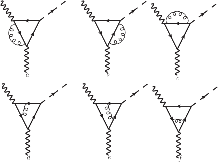
The lowest order QCD corrections include three vertex subgraphs and three quark self-energy subgraphs (Fig. 3). Kinematics of the main contributions of the Feynman triangle amplitude correspond to the ”almost on-mass-shell” quark connecting the ”almost on-mass-shell” photon and the emission of a real pion, while the two other quark lines are essentially off-mass-shell. Thus, one of the vertex function associated with the off-mass-shell external photon underlies the Sudakov conditions: both quarks are off-mass-shell. The two other vertices describe the situation when the photon and one of quarks are almost on-mass-shell, while the other quark is off-mass-shell. This configuration corresponds to the so-called Landau case [26]. The contribution from the triangle amplitude with a mass operator insertion to the ”almost real” quark line does not contain logarithmically enhanced terms.

Consider first the vertex subgraph with external highly virtual photon with momentum . The corresponding vertex function has the form (see Fig. 4a)
| (25) | |||||
| (26) |
Here, is a Casimir invariant of the SU(3) color group.
The logarithmically enhanced contributions arise from two kinematically different regions of virtual gluon momentum squared corresponding to small and large values of . Using the Sudakov parametrization
with light-like 4-vectors built from , we write in the limit (26), as
with
For the first term in the square brackets of we obtain (small region):
| (27) | |||||
where the factor 2 is due to the two regions of negative and positive values of the Sudakov parameters. In the derivation of (27), we used the relations , with being the Sudakov variables associated with the loop momentum of the quark loop.
The contribution from the region with large comes from the second term in the square brackets of
Here, we have to introduce the ultraviolet cut-off parameter , such as . The usual procedure of joining the denominators and performing the integration leads to
| (28) |
where Note, that we systematically omit the logarithmically suppressed terms. After regularization, the cut-off parameter must be replaced by the quark mass.
The total answer for is
| (29) |
The contribution of other Feynman amplitudes (Fig. 4b,c) does not contain logarithmic enhancement. We will illustrate this statement in the frame of QED [27, 26]. Let us consider the contribution of two remaining diagrams with one vertex function (Fig. 4b) and mass operator insertion (Fig. 4c)
| (30) | |||
Using the explicit expressions for the vertex and mass operator given in the Appendix, we obtain
where
We see, that the relevant contribution is suppressed by small factor . Other terms do not contribute to the amplitude. Similar statement is valid for two remaining diagrams (see Fig. 3 b,e).
Collecting all logarithmically enhanced contributions, we finally obtain
| (31) | |||||
Thus, the form factor at large (22), modified by next-to-leading (NLO) radiative QCD corrections, becomes
| (32) |
V Higher order QCD generalization
VI The results and discussion
There are two parameters within the parametrization of the pion transition form factor suggested by the quark model with radiative corrections. They are the quark mass and the strong coupling constant . We try to fit the experimental data for the form factor by varying these parameters. The results of the fit are presented in Tables 1-3 and Figs. 5-6.
In fitting procedure we use the parametrizations (2) and (5) as reference parametrizations. From corresponding goodness of fit (3), (4) and (6), (7) one concludes, first, that and, second, that the data set extended by experimental points of CELLO and CLEO and . The first fact is due to systematically lower error bars for the BaBar point set than for the Belle. The second property we interpret as indication on better consistency of the BaBar data with previous data at lower than for the Belle data11 1 At this point we disagree with conclusions made in [28]..
First of all, let us use our model to fit the BaBar and Belle data, considering the quark mass as a free parameter and the strong coupling to be fixed at , which corresponds to a renormalization scale of about 1 GeV. The results are given in Table I. For the leading order (LO) fit we use expression (22), for the next-to-leading order (NLO) fit we use expression (32), and the Sudakov resummed expression (Exp) is (34). In order to compare goodness of fit based on data used from different collaborations we introduce the relative parameter
| (35) |
with is for BaBar or Belle based data set. In (35), is for our model and for the power-like fits is from (3), (4) and (6), (7), correspondingly.
| BaBar | Belle | |||||
|---|---|---|---|---|---|---|
| [16] | [14] | |||||
| LO | 0.135 | 1.697 | 1.629 | 0.126 | 0.696 | 1.611 |
| NLO | 0.149 | 1.185 | 1.137 | 0.142 | 0.434 | 1.005 |
| Exp | 0.147 | 1.196 | 1.148 | 0.140 | 0.478 | 1.106 |
From Table 1 one finds that the goodness of the fit becomes better when going from the LO fit to the NLO fit, and almost does not change after Sudakov resummation. This justifies our model with radiative corrections. At the same time, the parameter becomes higher.
| BaBar+ | Belle+ | |||||
|---|---|---|---|---|---|---|
| [36] | [34] | |||||
| LO | 0.136 | 2.377 | 2.732 | 0.133 | 2.891 | 4.538 |
| NLO | 0.150 | 1.487 | 1.709 | 0.147 | 1.684 | 2.644 |
| Exp | 0.148 | 1.587 | 1.824 | 0.145 | 1.878 | 2.948 |
In Table 2 we made a fit of the BaBar and Belle data including also the set of points from CELLO and CLEO collaborations. We see that, qualitatively, for our model the situation does not change too much and the value of is practically the same for both cases. The later fact is rather important. It means that the fit procedure is basically related to the data points at intermediate in the region from 5 to 10 GeV2 where the data are more precise and consistent for all collaborations. At the same time, the region of higher (15-40 GeV2) is less important for the fit. The form factor in accordance with different parameterizations given in Table 2 is drawn in Figs. 5 and 6. In these figures we also present a power-like fits to the BaBar and Belle data (3) and (6), correspondingly.
| BaBar | Belle | |||||||
|---|---|---|---|---|---|---|---|---|
| [15] | [13] | |||||||
| NLO | 0.149 | 0.349 | 1.264 | 1.215 | 0.149 | 0.505 | 0.428 | 0.998 |
| Exp | 0.152 | 0.513 | 1.187 | 1.196 | 0.159 | 0.963 | 0.422 | 0.984 |
In Table 3 we made a two-parametric fit to the BaBar and Belle data. We see that such a two-parametric fit has equal or even lower with respect to corresponding numbers in Table 1. However, the price for that is a growing of the parameter especially for the case of Belle data. We consider such parametrization as not very physical.


VII Conclusions
In the present work we calculated the transition form factor of the neutral pion where one photon is virtual and another photon is real in the framework of the model where the light constituent quark mass and the quark-pion coupling are momentum independent22 2 Similar model was considered in [29, 30, 31] in view of calculations of hadronic corrections to the muon anomalous magnetic moment.. We generalize the previous leading order results [15, 18] obtained by considering the triangle diagram by including the radiative gluonic corrections to the first order in perturbation theory33 3 The problem of radiative corrections to the pion transition form factor was considered sometime ago in [32, 33, 34], within factorization approach with massless quarks. In this case the ”large logarithms” contain the QCD scale parameter .. The effect of higher order radiative corrections to the virtual photon vertex is estimated by applying the Sudakov exponentiation hypothesis. The results obtained are compared with existing experimental data on the pion transition form factor published by CELLO, CLEO, BaBar and Belle collaborations.
In general the model considered contains two parameters: the quark mass and the strong coupling constant .
First, we fit the data at fixed varying only . Taking into account the radiative corrections increases a little the fitting parameter up to MeV and improves a goodness of the fit. Considering separate fit of BaBar and Belle data (Table 1) one gets very close and the difference in is less than 10 MeV. Including also lower momentum data from CELLO and CLEO (Table 2) leads to inequality and almost coinciding . To our opinion it means that fitting procedure is most sensitive to the intermediate momentum interval, where both set of data are in agreement. As for parametrizations discussed in Introduction, BaBar data turns out to be more in accordance with lower momentum data than the Belle data. Our model is more close to the tendency of the BaBar data. Resummation effects do not lead to significant changes in goodness of the fit comparing with the NLO results.
Second, we try to fit data varying both model parameters (Table 3). The fit of data becomes better, especially in the region of large . However, has tendency to be close to unit. This fact is considered as not physically justified and thus not taken into account in our final results.
Let us emphasize that at the moment there are two sets of experimental data (BaBar and Belle) on the pion-photon transition form factor at high . They are fully consistent in the range of momentum transfer squared GeV2, but have different tendency at higher . Conditionally, the BaBar data show ”growing” behavior at large (see (2)), while the Belle data can be interpreted in twofold way as ”quasi-growing–quasi-constant” (see (2) and (5)). From experimental point of view, the data in the range GeV2 are consistent at the level of standard deviation. However, from theoretical point of view there are big debates on this difference [8, 9, 10, 11, 12, 13, 14, 15, 16, 17, 18, 19]. It is clear that only new high statistic experiments can resolve this problem.
The emergence of ”growing” data was so unexpected that, at first glance, it seemed that it is impossible to explain such behavior from the field theoretical point of view. However, in [15, 16, 17, 18, 19] there was noted that, if such ”growing” behavior exists, then it may be related to unusual properties of the pion distribution amplitude in the vicinity of its edge points. This behavior was conditionally called as ”flat”. In this case the inverse moment of the pion distribution amplitude is not well defined. In particular, such behavior may be modeled if to assume that the pion is almost structureless. In [15] (and later in some other works) it was shown that BaBar data can be described in the model with momentum independent quark mass and quark-pion coupling by using only one parameter: the constituent quark mass if its value is taken as MeV. This number was considered as a rather small from phenomenological point of view. One of the main motivation of the present work is to see how sensitive this parameter to gluonic radiative corrections, when fit the BaBar and Belle data. The result is that the mass parameter becomes a bit heavier MeV and the quality of the fit becomes better.
As it was shown in [19, 20], a more advanced model, with momentum dependent quark mass and quark-pion vertex, has the same qualitative features as the model considered in this work. In the model [19, 20], the soften quark propagator and quark-pion vertex lead to the single logarithmic asymptotic dependence on instead of the double logarithmic behavior, if the quark-pion vertex so that it corresponds to the ”flat” pion distribution amplitude. The pion distribution amplitude even can vanish at the end-points, but still simulate the logarithmic growth in rather wide range of momentum transfer including quite large values of it. When fit BaBar data, the mass parameter is still close to MeV. The calculations given in the present paper can be extended by consideration not only momentum dependent nonperturbative quark propagator and quark-pion vertex, but also momentum dependent nonperturbative gluon propagator.
Finally note that there are available data obtained by the BaBar collaboration for the , and transition form factors. The comparison of our model calculations with data for these mesons is given in [21]. From our point of view the data show tendency that with increase of the meson mass the form factor changes its behavior from the ”growing” regime to the ”constant” regime. In the framework of our model this change of behavior is related to strong dependence of the shape of the meson distribution amplitude on the meson mass. With growing meson mass the meson distribution amplitude changes its shape from the ”flat” one to the ”-function” shape for heavy mesons [21].
The study of present work shows that inclusion of the QCD corrections are essential in interpretation of experimental data on the pion transition form factor.
Acknowledgements.
We thank Yu.M. Bystritsky, V.V. Bytev, N.I. Kochelev and Yu.S. Surovtcev for their interest to the subject of present work and discussions. This work is supported in part by the Russian Foundation for Basic Research (project No. 11-02-00112).Appendix A Appendix
References
- [1] V. L. Chernyak and A. R. Zhitnitsky, JETP Lett. 25, 510 (1977).
- [2] G. P. Lepage and S. J. Brodsky, Phys. Lett. B87, 359 (1979).
- [3] A. V. Efremov and A. V. Radyushkin, Phys. Lett. B94, 245 (1980).
- [4] H. J. Behrend et al. [CELLO Collaboration], Z. Phys. C 49 (1991) 401.
- [5] J. Gronberg et al. [CLEO Collaboration], Phys. Rev. D57, 33 (1998), arXiv:hep-ex/9707031.
- [6] B. Aubert et al. [BaBar Collaboration], Phys. Rev. D80, 052002 (2009), arXiv:0905.4778.
- [7] S. Uehara et al. [Belle Collaboration], Phys. Rev. D 86 (2012) 092007 [arXiv:1205.3249 [hep-ex]].
- [8] S. V. Mikhailov and N. G. Stefanis, Nucl. Phys. B821, 291 (2009), arXiv:0905.4004.
- [9] S.J. Brodsky, F.-G. Cao and G.F. de Teramond, Phys. Rev. D84, (2011) 033001 [arXiv:1104.3364 [hep-ph]].
- [10] E. Ruiz Arriola and W. Broniowski, Phys. Rev. D81, (2010) 094021 [arXiv:1004.0837 [hep-ph]].
- [11] S. Noguera and V. Vento, Eur. Phys. J. A46 (2010) 197 [arXiv:1001.3075 [hep-ph]].
- [12] S.S. Agaev, V.M. Braun, N. Offen and F.A. Porkert, Phys. Rev. D83, (2011) 054020 [arXiv:1012.4671 [hep-ph]].
- [13] P. Kroll, Eur. Phys. J. C71 (2011) 1623 [arXiv:1012.3542 [hep-ph]].
- [14] Y. Klopot, A. Oganesian and O. Teryaev, Phys. Rev. D87, (2013) 036013 [arXiv:1211.0874 [hep-ph]].
- [15] A. E. Dorokhov, Phys. Part. Nucl. Lett. 7, 229 (2010), arXiv:0905.4577.
- [16] A. V. Radyushkin, Phys. Rev. D80, 094009 (2009), arXiv:0906.0323.
- [17] M. V. Polyakov, JETP Lett. 90, 228 (2009), arXiv:0906.0538.
- [18] Yu. M. Bystritskiy, V. V. Bytev, E. A. Kuraev and A. N. Ilyichev,Phys. Part. Nucl. Lett. 8 (2011) 73 [arXiv:0912.3668 [hep-ph]].
- [19] A. E. Dorokhov, JETP Lett. 92, 707 (2010).
- [20] A. E. Dorokhov, arXiv:1003.4693 [hep-ph].
- [21] A. E. Dorokhov, Nucl. Phys. Proc. Suppl. 225-227 (2012) 141 [arXiv:1109.3754 [hep-ph]].
- [22] V. V. Sudakov, Sov. Phys. JETP 3, 65 (1956).
- [23] S.B. Gerasimov, Yad. Fiz. 29 (1979) 513 [Sov. J. Nucl. Phys. 29 (1979) 259], JINR-E2-11693 (1979).
- [24] L. Ametller, L. Bergstrom, A. Bramon, and E. Masso, Nucl. Phys. B228, 301 (1983).
- [25] L. B. Okun, Leptons and quarks, Moscow, Science, 1981.
- [26] A. I. Akhiezr and V. B. Berestetskij, Quantum Electrodynamics, Moscow, Science, 1981.
- [27] E. A. Kuraev, N. P. Merenkov and V. S. Fadin, Yad. Fiz. 42 (1987) 782 [Sov. J. Nucl. Phys. 45 (1987) 486].
- [28] N. G. Stefanis, A.P. Bakulev, S. V. Mikhailov, A.V. Pimikov, arXiv:1202.1781 [hep-ph].
- [29] A. A. Pivovarov, Phys. Atom. Nucl. 66 (2003) 902 [Yad. Fiz. 66 (2003) 934] [hep-ph/0110248].
- [30] R. Boughezal and K. Melnikov, Phys. Lett. B 704 (2011) 193 [arXiv:1104.4510 [hep-ph]].
- [31] D. Greynat, E. de Rafael, JHEP 1207 (2012) 020 [arXiv:1204.3029 [hep-ph]].
- [32] F. del Aguila and M.K. Chase, Nucl. Phys. B193, (1981) 517.
- [33] E. Braaten, Phys. Rev. D28, (1983) 524.
- [34] E.P. Kadantseva, S.V. Mikhailov and A.V. Radyushkin, Yad. Fiz. 44 (1986) 507 [Sov. J. Nucl. Phys. 44 (1986) 326].