Active fluctuation symmetries
Christian Maes and Alberto Salazar, Instituut voor Theoretische Fysica
KU Leuven
12 November 2013
Abstract
In contrast with the understanding of fluctuation symmetries for entropy production, similar ideas applied to the time-symmetric fluctuation sector have been less explored. Here we give detailed derivations of time-symmetric fluctuation symmetries in boundary driven particle systems such as the open Kawasaki lattice gas and the zero range model. As a measure of time-symmetric dynamical activity over time we count the difference between the number of particle jumps in or out at the left edge and those at the right edge of the system. We show that this quantity satisfies a fluctuation symmetry from which we derive a new Green-Kubo type relation. It will follow then that the system is more active at the edge connected to the particle reservoir with the largest chemical potential. We also apply these exact relations derived for stochastic particle models to a deterministic case, the spinning Lorentz gas, where the symmetry relation for the activity is checked numerically.
1 Introduction
Fluctuation relations have emerged from an analysis of entropy production
in driven dissipative processes.
These are general and non-perturbative relations, something
which is not so common in nonequilibrium physics.
There has therefore been a big interest in such
fluctuation symmetries in recent decades, as pioneered in
the papers [1, 2].
It was found that such symmetries are an expression of local detailed balance,
implying that the total path-wise entropy flux is the source term of time-reversal breaking
in the nonequilibrium action governing the dynamical ensemble; see [3, 4, 5, 6, 7].
In turn, local detailed balance is implied by and refers to the underlying microscopic time-reversibility that governs the contact
between the system and each (equilibrium) reservoir in the environment [6, 8, 9, 10, 11, 12].
Also the nonequilibrium free energy relations, called Jarzynski
relation after [13], are of a very similar nature.
The present paper takes some distance from the original works. We do not concentrate on the traditional dissipative variables but we add a novel type of fluctuation symmetries belonging to the time-symmetric sector of a nonequilibrium system. That was already initiated in [14], but here we update our understanding with specific models and new Green-Kubo relations. Moreover, since then, a new wave of research interest on a specific time-symmetric quantity, the dynamical activity, has emerged [15, 16, 17, 18]. This dynamical activity, or frenesy as called in the context of linear response [18], captures essential nonequilibrium kinetic aspects. In the present paper differences in dynamical activity between the various contacts of the system with the environment arise from the breaking of a spatial symmetry that naturally accompanies the nonequilibrium situation. The main result of this paper (in Section 4) thus gives fluctuation symmetries in terms of a difference in dynamical activities.
For the plan of the paper, the next section formalizes the central idea. Besides time-reversal symmetry we add a second symmetry which can be spatial or internal and that gives rise to additional fluctuation symmetries. The standard example of a fluctuation symmetry for the entropy flux is then reviewed in Section 3. New to this case is the relation with the Kubo formula [19] (and not just the Green-Kubo relations) as it also follows from the fluctuation symmetry. We then concentrate on the boundary driven Kawasaki and zero range dynamics in Section 4. We derive in these models the active fluctuation symmetries for differences in dynamical activity (between the left versus right edge of the system). These give fluctuation–activity relations, also including a Green-Kubo relation for the mentioned dynamical activity. Interestingly, we are able to derive there that the activity (in terms of the number of particles moving in or out of the system) is highest at that side of the system which is in contact with the largest chemical potential. Section 5 applies the latter results to the spinning Lorentz gas, a mechanical model, where the notion of dynamical activity gets further realization in a classical physics context. The computer simulations we present validate our guesses also in the non-Gaussian fluctuation sector.
2 General observation
We start by presenting the formal content of fluctuation symmetries as in [3]. Let us denote quite generally a fluctuating quantity with the variable , where is the space of possible outcomes (e.g. path space). This means that the outcome of changes and is uncertain as, in physical terms, its value depends on hidden or more microscopic degrees of freedom. In addition we consider the presence of certain involutions and on , i.e., transformations which are equal to their inverse and that preserve the elementary structure of the space such as the volume element; these involutions are also mutually commuting: Id, . The fact that and are commuting ensures that is also an involution.
There will always be a reference probability law
for which is both and invariant;
.
11
1
For mathematical modeling purposes we consider probability distributions
for in . This in turn
also means that the space is measurable; in other words,
it supports some elementary structure
such as used for integration, so that probabilities
may admit a density function description.
Our main interest is to formulate a probability law on for the nonequilibrium process. We assume it has a density with respect to :
| (2.1) |
where the “action” on the paths or trajectories of the system appears. For our purposes, this action will be mostly explicitly known by setting a specific context. For the meaning and use of the nonequilibrium law (2.1), let us pretend for a moment that takes a finite number of values or states so that expectations under are simply written as finite sums
| (2.2) |
for an observable and with the probability that . Note for the notation that
denotes the random variable while stands for the different values it may take.
Now we present our general observation. Starting from (2.1) let us define on ,
| (2.3) | |||||
as functions of . In words, is the time-antisymmetric part of the action while is the time-symmetric complement. With this the action is expressed as
| (2.4) |
Note also that so that is the antisymmetric part of under when is antisymmetric under :
| (2.5) |
Observe that the very definitions (2.3) imply the following identities
| (2.6) | |||
| (2.7) |
for all functions on . From (2.7) we also have for symmetric observables such as that
| (2.8) |
We refer to (2.8) as an active fluctuation symmetry for reasons that will become clear in Section 4.
There is actually a rewriting of the relations above to the more familiar Gallavotti-Cohen type22 2 One uses this term refering to fluctuation relations which can be given as the logarithmic ratio of probabilities of opposite events. The possible connection with the asymptotic time limit will be explained shortly. fluctuation symmetries.
From (2.6) by taking the function we get
| (2.9) |
and, from (2.7) by choosing ,
| (2.10) |
with probabilities referring to the probability law .
Relations (2.7)–(2.8) are general and can be applied in a variety of ways. A new application will be established in Section 3.2 as well as in equations (3.19)–(3.21). Moreover, from (2.6) it follows that for all functions on ,
| (2.11) |
to first order in the action of (2.1) and where the last expectation is with respect to . The same holds replacing and in which case we would obtain fluctuation–activity relations.
Another consequence is that always and . These inequalities are not only useful to determine the direction of currents (the more standard application) but, as we will see, enable to predict at what side of a boundary driven system the activity is largest, which is an entirely new application.
Let us emphasize that the results above are exact, i.e., valid for all times.
All the consequences mentioned
will remain basically intact also for variables that
differ from or by a total (time-)difference as long as some boundedness
of that difference can be assured.
If so, we will get asymptotic fluctuation symmetries, where (2.6)–(2.10)
are not exact for the variables but only valid in some limit (of large observation time).
Such asymptotic formulæ would correspond to stationary fluctuation theorems as in [2].
Further, the relevance of the fluctuation identities (2.6)–(2.7) depends crucially on the systematic and operational meaning of and . It was understood before that is deeply related to changes in entropy (as we will briefly repeat in the next Section); in Sections 4–5 we treat a number of examples where is made visible and related to the dynamical activity.
3 Standard example: entropy flux
The present section contains the standard application of (2.6) to obtain a fluctuation symmetry for the total entropy flux in nonequilibrium Markov jump models. The reader will only find as new some reflections towards the end of the section connecting the fluctuation symmetry also with response theory and the Kubo formula. Nevertheless examples for spatially extended systems are not so common in the literature on fluctuation symmetries and the present section treats them in a still less familiar but unifying framework.
Consider a Markov jump process on a finite state space . We specify the transition rates (time-dependent) for jumps between system states
| (3.1) |
where is a time-dependent (external) protocol changing the function . is called the energy of the system when it is found at state with external value ; this is because we imagine that the changes in are exactly balanced by the change of energy in the environment. The driving is antisymmetric but it does not need to be a total difference for all , which is important to model nonequilibrium features. The reactivities are symmetric. The additional time-dependent parameter in (3.1) is the varying inverse temperature of the environment (in units where ). Note that the nonequilibrium driving sits entirely in the function (which contains the irreversible work) and in the time-dependence of both the protocol and the inverse temperature . Clearly, if and when are constant, then the process is reversible with stationary distribution .
It is important to note that both the form and the interpretation of (3.1) follow from the condition of local detailed balance, for which at all times (and always with )
| (3.2) |
is the entropy flux in the transition ; that is the change of entropy in the environment. This explains the standard origin of the exponential form of the rates and in particular why the antisymmetric term contributes to the irreversible work; see also below in (3.8) and in the examples of Section 4.1.
For a given path over the time-interval the energy change is given by
| (3.3) |
where the sum is made for the transitions occurring at the jump times , and denotes the state of the system right before the jump to .
In equation (3.3) we have two effects for the energy change. Firstly, for fixed value the system state has changed and then energy is exchanged with the environment as heat
| (3.4) |
(again the sum is made over jump times in ). Secondly, for fixed state the external value changes , doing work
| (3.5) |
Thus, equation (3.3) mimics the first law of thermodynamics. The energy change of the system equals the change in internal energy received as heat from the environment plus the amount of work done on the system by the environment:
| (3.6) |
The nonequilibrium driving can be added and subtracted from this balance. We think of it as doing work on the system, which is instantaneously released as heat, so that now , but with
| (3.7) |
with all terms depending on a specific path . We refer to [21] for more details and insights on stochastic energetics.
In the same spirit we can also associate a change in entropy of the environment to a path or trajectory . The idea is that the environment consists of big equilibrium reservoirs undergoing only reversible changes in interaction with the system. One looks back at (3.4) and (3.7) to define
| (3.8) |
for the change of the entropy in the environment (always per ). This term is the total entropy flux for trajectory , which can be split into a reversible part, due to the energy exchange, and an irreversible part
| (3.9) |
Particular examples such as the one treated in Section 4.1 will present explicit expressions for the driving , as in equations (4.3)–(4.4). The examples treated will also clarify further its connection to irreversibility, which as will be seen in the models sits exclusively at the boundaries.
We now repeat the observation of [3, 6] that the entropy flux (3.8) can be obtained as for (2.6)
as the source term of time-reversal breaking.
Let us leave out the kinematical time-reversal on and proceed with the undecorated time-reversal , which is defined on trajectories in phase space or paths via for . One can check from (3.8) that the entropy flux per path is antisymmetric under time-reversal, . Let now denote the path distribution when we start at time zero from a probability law on . The time-dependence of the protocol can be reversed to define . We choose a second probability law on for starting the latter (protocol-reversed) Markov process, with path-distribution denoted by . Assuming and that implies (dynamical reversibility), we can find the in (2.6) via
| (3.10) |
and find
| (3.11) |
for jump times in . Indeed the jump times in the reversed trajectory are respectively . One can see what (3.11) becomes for the rates (3.1). Substituting into the previous formula makes
| (3.12) |
which is (3.8). That relation can be called a (generalized) Crooks relation [5], and for it almost immediately produces Jarzynski identities which are used to evaluate equilibrium free energies from the fluctuations of the dissipative work — we refer to the literature and the references therein for more details, [13, 22, 7].
Let us now specify to the case where are constant in time. In particular, with respect to (3.9), and for state functions , we have the identity
| (3.13) |
for all trajectories . Note that the left-hand side is defined from (3.10) implementing (2.6), while the right-hand side is defined from the heat and (3.8)–(3.9). Therefore, the identities (3.12)–(3.13) are the core of what is generally called the fluctuation symmetry, the fluctuation relations or the fluctuation theorem (transient or steady state, as recalled also at the end of Section 2) for the entropy production.
3.1 Exact fluctuation symmetry
In the following we restrict ourselves to time-homogeneous Markov processes and we do no longer write the dependence on . We take also inverse temperature .
Consider the reference reversible process started in equilibrium for which there is detailed balance with rates
| (3.14) |
The nonequilibrium process has rates and we choose to start it also from . Its distribution on paths in the time-interval is then denoted by . We proceed as in (2.3) to find
| (3.15) |
for escape rates . Now clearly (2.6) holds, and with for all , we have the exact fluctuation symmetry
| (3.16) |
with expectations in the nonequilibrium process starting from the equilibrium distribution . That result in itself is of course not new and has been derived in various ways; see e.g. equation (2.32) in [3] or equation (3.34) in [23].
Another way to get an exact fluctuation symmetry is to look back at (3.13) with probabilities equal to the stationary distribution of the nonequilibrium process. We then have by combining (3.10) with (3.13) that in the nonequilibrium steady regime, for all ,
| (3.17) |
for irreversible entropy flux and with state function . The exact symmetry (3.17) would invite us to give special physical meaning also to that function , but no convincing thermodynamic or operational meaning exists. Only in some cases like the models we treat in Sections 4.2–5, this physical interpretation of in (3.17) can be made. This is also why asymptotic (in ) fluctuation symmetries, obtained from (3.17) for any positive function of , have been more appreciated. These asymptotic fluctuation formulas are obtained by taking the logarithm of both sides in (3.17) and dividing them by ; then using the boundedness of the function will make it disappear when finally letting .
3.2 Relation to linear response
Looking backward, it appears that the main input has been relation (3.12). That has analogues for diffusion process [4, 24, 25], for dynamical systems [2, 29, 26, 27] and also for non-Markovian processes [3, 28, 30] as long as there is sufficient space-time locality to ensure a large deviation principle [3]. The main origin of the fluctuation symmetry is therefore the identification of the entropy flux as marker of time-reversal breaking, [29, 3, 5, 6].
Quite some features of the close-to-equilibrium regime are easily deduced from the fluctuation symmetry. There are for example the Green-Kubo relations, with Onsager reciprocity as first explained in [31] following from an extended fluctuation symmetry. More globally, the validity of the McLennan ensemble close-to-equilibrium is another implication, see [32, 33].
We illustrate just one aspect which we have not seen stated as such, and which is useful. Start again from (2.6) and take a function in terms of another function of interest. Then,
| (3.18) |
Imagine now that the action in (2.1) is small, so that the law is just a small perturbation of the reference law and so that is small. We can then expand the last term in (3.18) to bring
| (3.19) | |||||
where the last expectation, with the subscript , is with respect to the reference and we have used that is invariant. That linear order relation can be applied to the context of dynamical ensembles as we had it above, with being time-reversal on trajectories . Take for example the particular case where so that for a state function ; are the initial and final states of the trajectory , respectively. We then obtain from (3.19) the linear response formula
| (3.20) |
where the expectations refer to the process started from equilibrium at time zero. In order to recognize the Kubo formula one should substitute in (3.20) the expression (3.12) for with , and being the equilibrium distribution with potential . Then, still using the first law (3.3), we arrive at the more familiar Kubo expression
| (3.21) | |||||
Yet, it takes the combination (3.12)–(3.20) to immediately understand why this formula
is truthfully called fluctuation-dissipation relation.
Moving beyond the linear response around equilibrium makes it more difficult to find specific consequences. Of course, the fluctuation relations hold unperturbed but there is no direct way to derive more specific results. In fact, it appears that one really needs more information about the time-symmetric part, in (2.3), to move further [20, 34]; that is also part of the motivation of the next sections.
4 Symmetry in dynamical activity
We come to give examples of the fluctuation symmetry (2.7), referred to in the title of the paper as active because they deal with the dynamical activity.
4.1 Boundary driven Kawasaki dynamics
We consider a system of indistinguishable particles subject to exclusion on a lattice interval which is boundary driven. The state space is , where states are particle configurations , interpreted as vacant versus occupied sites on a lattice interval. The dynamics has two parts. First, there is a bulk exchange of neighboring occupations with rate given, for inverse temperature ,
| (4.1) |
when for all except for for some . The interaction between neighboring sites is ruled by the potential
| (4.2) |
where is the coupling parameter; note that the case corresponds to the symmetric exclusion process.
Second, apart from the interacting diffusion part to the dynamics above, there are also the reactions at the boundary sites where creation and annihilation of particles take place
| (4.3) |
for except for , the boundaries, where with and . Besides
| (4.4) | |||||
where for one has and for some fixed parameters . The physical interpretation of this birth and death process is the contact at the boundaries with particle reservoirs at left and right chemical potentials , respectively.
For all other transitions we have . As a result,
| (4.5) |
with (number of particles in the system for state ), and with current
| (4.6) | |||||
and zero otherwise. In other words, with the current of particles into the left reservoir and the current of particles into the right reservoir for the transition .
For (and only for ) there is detailed balance with grand-canonical ensemble
| (4.7) |
In this case the parameter is the chemical potential of both particle reservoirs left and right. That equilibrium process determines our reference distribution . Nonequilibrium arises from taking , which makes the chemical potentials in the imagined left and right particle reservoirs different. We can start the nonequilibrium process from the same , giving our distribution , but asymptotically in time a nonequilibrium steady regime will develop. In particular it is easy to prove now that for there will be a steady particle current from left to right. See for example [35] for the details of the standard fluctuation symmetry as in the previous section.
The decomposition (2.3) here gives
| (4.8) |
with for time-reversal, and the net number of particles that escape from the lattice interval to the left particle reservoir. Note that , the change of the number of particles in the system.
For the time-symmetric part of the action we can compute, from (3.15)
| (4.9) |
where (putting now for notational simplicity)
again for and . Next, in order to obtain the symmetry in the dynamical activity, we apply the mirror transformation through which . Observe that in that mirror symmetry . We can thus compute
| (4.10) |
from the expected difference in transitions (jumps in and out of the system) left versus right, to find
| (4.11) | |||||
which is of course also odd in the driving field . Now for the boundary driven symmetric exclusion process we must take the coupling , and in (4.11) only survive
| (4.12) |
which is given entirely in terms of the difference in occupations at the outer sites.
It follows from the general analysis in Section 2 that in (4.10) verifies the fluctuation symmetries (2.7)–(2.10). This is a non-trivial general identity whose meaning refers to the reflection-antisymmetric part in the dynamical activity (4.9). In particular, that identity (2.7) for that same in (4.10)–(4.11) remains strictly valid even when modifying the interaction potential in the bulk of the system. On the other hand, applying the general consequence that , or , to (4.12) only gives the well known fact that the density is larger (for constant temperature) at the side of the largest chemical potential.
4.2 Boundary driven zero range process
We now discuss the application of fluctuation symmetries to a bosonic version of the previous example, where particles diffuse without exclusion principle.
Consider again a one-dimensional channel composed of cells in which we observe occupation numbers , . The particle configuration can change in two ways. In the first place, it changes at a rate via bulk hopping, , where stands for the particle configuration with one particle in cell and zero elsewhere. The choice corresponds to independent particles. Secondly, at the boundaries, the channel is connected to left/right particle reservoirs with chemical potentials and , respectively. The transition rates for the creation/annihilation of particles at the two sites are then
| (4.13) |
with . The rates for these transitions evoke the chemical potentials at the boundary walls from . We assume that so that, for , we have the equilibrium situation where the chemical potentials left and right become equal. Of course we could have chosen also to modify the exit rates but it appears physically most accessible to change the incoming rates to achieve a nonequilibrium regime, as we also do in the next section. In fact, to make the equilibrium left/right symmetric we also take . The corresponding stationary distributions (at ) and (at general ) are product distributions but that will not be used in the following.
Consider the trajectories . Both equilibrium and nonequilibrium processes start from the same equilibrium distribution . The action (2.1) is easily calculated to be
| (4.14) |
where e.g., indicates the number of particles entering the system from the left reservoir for the path . As we apply time-reversal , we obtain the time anti-symmetric part of the action
| (4.15) | |||||
where now e.g., is the net number
of particles that have escaped
to the left particle reservoir during .
As usual and as explained before, that entropy production satisfies the exact fluctuation symmetry (2.9).
For the asymptotic form, one must be more careful because of the unbounded number of particles; see [36].
Here we are however more interested in the dynamical activity.
Let us then look at the time-symmetric term ,
| (4.16) |
This is the analogue to (4.9), for the Kawasaki dynamics example. Thus, as we did in Section 4.1, we will apply the mirror transformation , reversing left/right. First note that here again the entropy is antisymmetric under , . On the other hand, we have
| (4.17) |
exactly proportional to the difference in dynamical activity between the right and left boundaries,
| (4.18) |
Following the logic of (2.7), that suffices for a variable to satisfy a fluctuation symmetry (2.10) up to a total time-difference. Even more, when the observable is time-symmetric, then
| (4.19) |
for all times , where we start the nonequilibrium process at time zero from . For example taking , to first order in ,
| (4.20) |
which is formally similar to a Green-Kubo relation [31, 19] but now the observable in (4.18) is time-symmetric.
It is in fact true for all that , which means that the greatest activity is to be found at the boundary side of the largest chemical potential. In other words, as for the boundary driven Kawasaki dynamics also for zero range, the particle current can be said to be directed away from the region of largest activity. These statements all hold for any form of the bulk rate and are quite independent of the usual statements involving the fluctuation symmetry of entropy production or currents.
5 Spinning Lorentz Gas
The spinning Lorentz gas (SLG) is a classical mechanical model of particle scattering in 2D;
it is actually an interacting version of the normal Lorentz gas [37], which is
a well known example of deterministic particle diffusion [38, 39]. The SLG has
the additional feature of providing local thermalization of the wandering particles along
with the scatterers; a complete description of this and the coupled energy and
mass transport properties of the SLG model can be found in [40]. As a matter of fact,
the validity of the fluctuation theorem for the entropy production (Eqn. (2.9)) and for
the joint distribution of currents has been tested for this model, of course taking
into account the limitations due to the unbounded kinetic energy, see [41].
Also, a precise meaning to the state function , mentioned after (3.17), can be found in
the SLG model for the exact symmetry case, which is then taken to the asymptotic limit
where vanishes [41].
As illustrated in Fig. 1, the array of scatterers is connected to
thermo-chemical reservoirs, with chemical potentials and at inverse temperatures .
This setting drives the system into a nonequilibrium stationary regime when .

The SLG is a microscopic mechanical model which we want to connect with the boundary
driven zero range model of the previous section.
In order to do this, note first that only at the walls in Fig. 1
point particles can enter and leave the system. The rates at which new
particles enter are related to the mean density
of their reservoir as , an effusion process;
see also [42].
We focus in a nonequilibrium setting of the SLG where there is
a reservoir chemical potential difference, given by
; hence,
in the notation of the previous section we have .
The hypothesis to be tested here is that identical fluctuation relations as (2.7)–(2.10) hold for the dynamical activity in the SLG as we had it for the boundary driven zero range process before, particularly in the version (4.19). One therefore looks back at the expression (4.17). More precisely, we look at the fluctuations of the time-symmetric variable
| (5.1) |
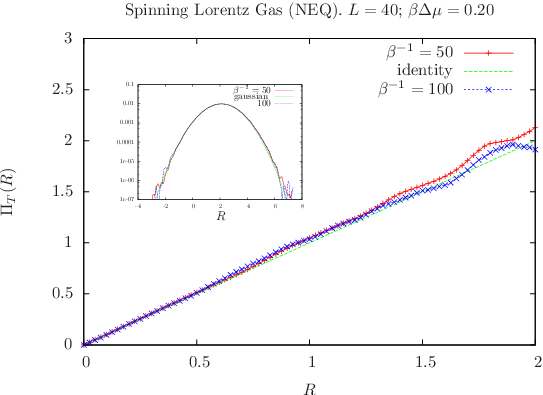
We have measured in molecular dynamics simulations of the SLG model the probability distribution , in stationary nonequilibrium. Figs. 2 and 3 show the validation of the time-symmetric fluctuation theorem for . In these figures, to test the fluctuation symmetry we plot, as usual, the functional
| (5.2) |
The measuring time was a
large value of ; in the same time units,
the average time between collisions in the gas is .
In the first nonequilibrium case (Fig. 2) the stationary state
is obtained by a chemical potential difference
between the reservoirs, and for two different temperatures.
The second case (Fig. 3) corresponds to a
larger driving ; this gives a fluctuation theorem
interval in which the distribution is visibly non-Gaussian.
The variable (5.1) gives the fluctuations in the difference of dynamical activity at sites . As in the remark around (4.12), here the dynamical activity in (5.1) is proportional to the number of transitions at each of the walls; in other words, it is proportional to the local boundary density. Since the temperature in this case is uniform, the activity fluctuations are simply related to density fluctuations of the stationary profiles. Thus, when measuring the differences in dynamical activity in (5.1) one obtains asymmetric statistics arising from the density profile in the slab, which is shaped by the nonequilibrium condition set by the reservoirs.

6 Summary
We have discussed a general framework to derive Gallavotti-Cohen type fluctuation relations based on symmetry transformations applied to the dynamical ensemble. We have shown that the time-antisymmetric sector contains the more usual fluctuation relations for the entropy production, with time reversal as the fundamental symmetry. In the other hand, fluctuation symmetries for time-symmetric variables involve a different phenomenology, dealing with non-dissipative variables. The present paper indeed emphasizes the relevance of this less studied and complementary time-symmetric fluctuation sector of the non equilibrium process. For this an extra symmetry is involved, most simply a mirror or reflection symmetry, which basically is equivalent to reversing the driving field. This task leads to fluctuation symmetry relations for differences in the dynamical activity, as we have illustrated with three examples of boundary driven systems. Interestingly, one finds that new Green-Kubo relations for the activity hold, and we understand where in some spatially extended system the activity is maximal.
The fact that the same time-symmetric fluctuation symmetry
remains verified for models
like the spinning Lorentz gas, which is deterministic, chaotic and interacting,
indicates further the more universal validity of
this class of active fluctuation symmetries.
Acknowledgment Financial support in the form of a Belgian InterUniversity Grant from Belspo is gratefully acknowledged.
References
- [1] D.J. Evans, E. G. D. Cohen and G.P. Morris, Probability of second law violations in steady flows. Phys. Rev. Lett. 71, 2401–2404 (1993).
- [2] G. Gallavotti and E. G. D. Cohen, Phys. Rev. Lett. 74, 2694 (1995); J. Sat. Phys. 80, 931 (1995).
- [3] C. Maes, The fluctuation theorem as a Gibbs property. J. Stat. Phys. 95, 367–392 (1999).
- [4] J.L Lebowitz and H. Spohn, The Gallavotti–Cohen fluctuation theorem for stochastic dynamics. J. Stat. Phys. 95, 333 (1999).
- [5] G. E. Crooks, Entropy production fluctuation theorem and the nonequilibrium work relation for free energy differences. Phys. Rev. E 60, 2721–2726 (1999).
- [6] C. Maes and K. Netočný, Time-reversal and Entropy. J. Stat. Phys. 110, 269–310 (2003).
- [7] C. Maes, On the origin and the use of fluctuation relations for the entropy. Séminaire Poincaré 2, 29–62 Eds. J. Dalibard, B. Duplantier and V. Rivasseau, Birkäuser (Basel), 2003.
- [8] P.G. Bergman and J.L. Lebowitz, New Approach to Nonequilibrium Process. Phys. Rev. 99, 578-587, 1955.
- [9] S. Katz, J.L. Lebowitz, and H. Spohn, Stationary nonequilibrium states for stochastic lattice gas models of ionic superconductors. J. Stat. Phys. 34, 497–538 (1984).
- [10] T. Harada and S.-Y. Sasa: Equality connecting energy dissipation with violation of fluctuation-response relation, Phys. Rev. Lett. 95, 130602 (2005).
- [11] B. Derrida, Non-equilibrium steady states: fluctuations and large deviations of the density and of the current. J. Stat. Mech. P07023 (2007).
- [12] H. Tasaki, Two theorems that relate discrete stochastic processes to microscopic mechanics. arXiv:0706.1032v1 [cond-mat.stat-mech].
- [13] C. Jarzynski, Phys. Rev. Lett. 78, 2690 (1997); Phys. Rev. E 56, 5018 (1997).
- [14] C. Maes and M.H. van Wieren, Time-symmetric fluctuations in nonequilibrium systems. Phys. Rev. Lett. 96, 240601 (2006).
- [15] R. Jack, J.P. Garrahan, D. Chandler: Space-time thermodynamics and subsystem observables in kinetically constrained models of glassy materials, J. Chem. Phys. 125, 184509 (2006).
- [16] J. P. Garrahan, R.L. Jack, V. Lecomte, E. Pitard, K. van Duijvendijk, and F. van Wijland: First-order dynamical phase transition in models of glasses: an approach based on ensembles of histories, J. Phys. A: Math. Gen. 42, 075007 (2009).
- [17] W. De Roeck and C. Maes, Symmetries of the ratchet current. Phys. Rev. E 76, 051117 (2007).
- [18] M. Baiesi, E. Boksenbojm, C. Maes and B. Wynants, Nonequilibrium linear response for Markov dynamics, I: jump processes and overdamped diffusions, J. Stat .Phys. 137, 1094-1116 (2009).
- [19] R. Kubo, The fluctuation-dissipation theorem. Rep. Prog. Phys. 29, 255-–284 (1966).
- [20] M. Colangeli, C. Maes and B. Wynants, A meaningful expansion around detailed balance. J. Phys. A: Math. Theor. 44, 095001 (2011).
- [21] K. Sekimoto, Stochastic Energetics. Lecture Notes in Physics 799, Springer (2010).
- [22] F. Ritort, C. Bustamente and I. Tinoco,Jr., A two-state kinetic model for the unfolding of single molecules by mechanical force. Proc. Nat. Ac. Scienc. 99, 13544-–13538 (2002).
- [23] R. J. Harris and G. M. Schütz, Fluctuation theorems for stochastic dynamics, J. Stat. Mech: Theory and Experiment, P07020 (2007).
- [24] J. Kurchan, Fluctuation theorem for stochastic dynamics. J. Phys. A: Math. Gen. 31, 3719-–3729 (1998).
- [25] C. Maes, F. Redig and A. Van Moffaert, On the definition of entropy production, via examples. J. Math. Phys. 41, 1528-1554 (2000).
- [26] D. Ruelle, Smooth Dynamics and New Theoretical Ideas in Nonequilibrium Statistical Mechanics. J. Stat. Phys. 95, 393-–468 (1999).
- [27] C. Maes and E. Verbitskyi, Large deviations and a fluctuation symmetry for chaotic homeomorphisms. Comm. Math. Phys. 233, 137–151 (2003).
- [28] D. Andrieux and P. Gaspard, The fluctuation theorem for currents in semi-Markov processes. J. Stat. Mech.:Theory and Experiment, P11007 (2008).
- [29] F. Bonetto, G. Gallavotti, and P. Garrido, Chaotic principle: An experimental test. Physica D 105, 226 (1997).
- [30] C. Maes, K. Netočný and B. Wynants, Dynamical fluctuations for semi-Markov processes. J. Phys. A: Math. Theor. 42, 365002 (2009).
- [31] G. Gallavotti, Extension of Onsager’s Reciprocity to Large Fields and the Chaotic Hypothesis. Phys. Rev. Lett. 77, 4334–4337 (1996).
- [32] T. S. Komatsu and N. Nakagawa, An expression for stationary distribution in nonequilibrium steady states. Phys. Rev. Lett. 100, 030601 (2008).
- [33] C. Maes and K. Netočný, Rigorous meaning of McLennan ensembles. J. Math. Phys. 51, 015219 (2010).
- [34] C. Maes, K. Netočný, and B. Wynants, On and beyond entropy production; the case of Markov jump processes. Markov Proc. Rel. Fields. 14, 445–464 (2008).
- [35] C. Maes, K. Netočný and B. Shergelashvili, A selection of nonequilibrium issues. In: Methods of Contemporary Mathematical Statistical Physics, Ed. Roman Kotecký, Lecture Notes in Mathematics 1970, pp. 247-306, Springer, 2009.
- [36] R. J. Harris, A. Rákos and G.M.Schütz, Breakdown of Gallavotti-Cohen symmetry for stochastic dynamics. Europhys. Lett. 75, 227 (2006).
- [37] H. A. Lorentz, Proc. Amst. Acad. 438 (1905).
- [38] P. Gaspard, Chaos, Scattering, and Statistical Mechanics (Cambridge University Press, Cambridge, 1998).
- [39] Hard Ball Systems and the Lorentz Gas, edited by D. Szász (Springer Verlag, Berlin, 2000).
- [40] H. Larralde, F. Leyvraz and C. Mejia-Monasterio, Transport properties of a modified Lorentz gas. J. Stat. Phys. 113, 197–231 (2003).
- [41] A. Salazar, F. Leyvraz and H. Larralde, Fluctuation theorem for currents in the Spinning Lorentz Gas. Physica A 388, 4679–4694 (2009).
- [42] F. Reif, Fundamentals of Statistical and Thermal Physics (International Student Edition), McGraw-Hill, Tokyo, 1965; pp. 272.