Practical Implementation of Spatial ModulationThanks: Copyright (c) 2013 IEEE. Personal use of this material is permitted. However, permission to use this material for any other purposes must be obtained from the IEEE by sending a request to pubs-permissions@ieee.org. Thanks: The associate editor coordinating the review of this paper and approving it for publication was Prof. Yong Liang Guan. Manuscript received October 2, 2012; revised February 18, 2013 and April 24, 2013. Thanks: N. Serafimovski, A. Younis, P. M. Grant and H. Haas are with The University of Edinburgh, Edinburgh, EH9 3JL, UK, (e–mail: {n.serafimovski, a.younis, p.grant, h.haas}@ed.ac.uk.). Thanks: M. Di Renzo is with the Laboratoire des Signaux et Systèmes, Unité Mixte de Recherche 8506, Centre National de la Recherche Scientifique–École Supérieure d’Électricité–Université Paris–Sud XI, 91192 Gif–sur–Yvette Cedex, France, (e–mail: marco.direnzo@lss.supelec.fr). Thanks: R. Mesleh is with the Electrical Engineering Department and SNCS research center, University of Tabuk, P.O.Box: 71491 Tabuk, Saudi Arabia, (e–mail: rmesleh.sncs@ut.edu.sa). Thanks: P. Chambers and C.-X. Wang are with Heriot-Watt University, Edinburgh, EH14 4AS, UK. (e–mail: {P.Chambers, Cheng-Xiang.Wang}@hw.ac.uk). Thanks: M. A. Beach is with The University of Bristol, Bristol, BS8 1UB, UK. (e–mail: M.A.Beach@bristol.ac.uk) Thanks: Digital Object Identifier 00.0000/TVT.0000.00.000000
Abstract
In this work we seek to characterise the performance of SMlow (SMlow) and SMX (SMX) with an experimental testbed. Two National Instruments (NI)-PXIe devices are used for the system testing, one for the transmitter and one for the receiver. The digital signal processing that formats the information data in preparation for transmission is described along with the digital signal processing that recovers the information data. In addition, the hardware limitations of the system are also analysed. The aber (aber) of the system is validated through both theoretical analysis and simulation results for SMlow and SMX under LoS (LoS) channel conditions.
Index Terms:
Spatial Modulation (SM), Spatial Multiplexing (SMX), Multiple–Input Multiple–Output (MIMO) systems, Experimental Results, Wireless TestbedI Introduction
Multiple–input multiple–output (MIMO) systems offer a significant increase in spectral efficiency in comparison to single antenna systems [1, 2]. An example is SMlow, which increases the spectral efficiency of single antenna systems while avoiding ICIlow (ICIlow) [3]. This is attained as shown in Fig. 1, through the adoption of a new modulation and coding scheme, which foresees: i) the activation, at each time instance, of a single antenna that transmits a given data symbol (constellation symbol), and ii) the exploitation of the spatial position (index) of the active antenna as an additional dimension for data transmission (spatial symbol) [4]. Both the constellation symbol and the spatial symbol depend on the incoming data bits. An overall increase by the base–two logarithm of the number of transmit–antennas of the spectral efficiency is achieved. This limits the number of transmit antennas to be a power of two unless FBE--SM (FBE--SM) [5], or gsm (gsm) [6] are used. In particular, in [6] it is shown that the number of spatial symbols does not need to be equal to the number of transmit antennas. For example, if gsm is used, the number of spatial symbols is equal to the number of unique channel signatures between the transmitter and receiver, where the unique channel signatures can be obtained by activating various combinations of the available transmit antennas. In this work, however, these unique channel signatures are assumed to be due to the activation of individual transmit antennas.


Activating only one antenna at a time means that only one RF chain is needed, which significantly reduces the hardware complexity of the system [7]. Moreover, the most energy consuming part of a base station are the power amplifiers and the RF (RF) chains associated with each transmitter [8], where the power requirements of a base station are shown to increase linearly with the number of RF chains added [9]. However, as only one RF chain is needed, SM offers a reduction in the energy consumption which scales linearly with the number of transmit antennas [10, 11]. Furthermore, the computational complexity of SM–ML is equal to the complexity of single–input multiple–output (SIMO) systems [12], i.e. the complexity of SM–ML depends only on the spectral efficiency and the number of receive antennas, and does not depend on the number of transmit antennas. Moreover, in [13, 14, 15], the complexity of SMlow is further reduced by using the SD (SD).
Several papers that seeks to understand and hence improve the performance of SMlow in various scenarios are available in literature. In [16, 17], the aber performance of SMlow is improved by introducing trellis coding on the transmitting antennas. The optimal detector is derived with and without channel state information at the receiver in [12, 18, 19]. The aber performance is given when considering channel estimation errors in [20, 21, 22]. The optimal power allocation for the case of two transmit antennas and one receive antenna system is given in closed form in [23], and the aber performance of SMlow in correlated fading channels is considered in [24]. In [25, 26] spectral efficiency and diversity gains are obtained by combining SMlow with space-time block codes (STBC–SM). Applying SMlow to relaying systems is also shown to result in significant snr (snr) gains when compared to non-cooperative decode and forward techniques [27]. In [28] the overall power performance of a bs (bs) employing SMlow is studied. More recently, a comprehensive analytical framework to compute the aber of SMlow over generalized fading channels is introduced in [29]. Moreover, in [30] for the first time the performance of SMlow is analysed using real–world channel measurements. The latest research achievements and an outline of some relevant open research issues for SMlow are reviewed in [31]. All research thus far is strictly theoretical.
In this paper, the aber performance of SMlow is analysed in a practical testbed and compared with that for SMX. In particular, the ni (ni)–PXIe–1075 chassis are used at the transmitter and receiver. The design of the testbed hardware and the software used are explained in detail along with the transmission chain. The effects of the entire transmission chain on the system performance are examined. The basic elements of the transmission link are the transmit RF chain, the wireless channel, and the receive RF chain. In addition to the effects of the wireless channel on the phase and amplitude of the signal, the impact on the system performance of the power imbalances (PIs) in the transmitter and receiver RF chains is discussed. Furthermore, an analytical upper bound for the aber performance of SMlow over NLoS (NLoS) channels with pim (pim) is derived, and compared to the experimental and computer simulation results. The experimental results validate the analytical bound as well as the attained computer simulations. Finally the performance of SMlow is compared with the theoretical and experimental results of SMX.
This paper is organised as follows. The system set-up, equipment and digital signal processing are presented in Section II. The equipment constraints are then considered in Section III, while the analytical modelling is discussed in Section IV. In addition, the computational complexity of the SMlow decoder algorithm is presented in Section V. The performance of SMlow is then characterised in the experimental and simulation environments in Section VI, where it is compared with the theoretical and experimental results of a SMX system. Lastly, the paper is summarised in Section VII.
II Testbed Set–up and System Model
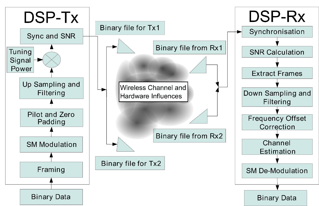
The testbed set–up and transmission chain can be separated into software and hardware parts, as shown in Fig. 2. The hardware consists of the PXIe--Tx (PXIe--Tx) and the PXIe--Rx (PXIe--Rx). The software consists of the DSP--Tx (DSP--Tx) and the DSP--Rx (DSP--Rx).
The binary data to be broadcast is first processed by DSP--Tx, before being transmitted through the fading channel by the PXIe--Tx. The channel coefficient on the link between transmit antenna , and receive antenna , is denoted by . Note that the number of antennas at the transmitter and the receiver are denoted by and , respectively. At the receiver, the PXIe--Rx records the RF signal and passes it through to the DSP--Rx for processing, where the original data stream is recovered.
II-A Testbed Hardware
The NI–PXIe–1075 chassis are equipped with a GHz Intel–i processor with GB RAM and are shown in Fig. 3. The system has two transmit antennas and two receive antennas. Each antenna at the transmitter and receiver contains two quarter–wave dipoles, and one half–wave dipole placed in the middle. All three dipoles are vertically polarised. In addition, each antenna has a peak gain of dBi in the azimuth plane, with an omnidirectional radiation pattern.
II-A1 Transmitter hardware (PXIe–Tx)
The following NI–PXIe modules are used at the transmitter,
- •
NI-PXIe-5450 16-Bit I/Q Signal Generator (SG–16bit),
- •
NI-PXIe-5652 RF Signal Generator with a kHz to GHz frequency range (SG–RF),
- •
NI-PXIe-5611 intermediate frequency (IF) to carrier RF up–converter (up–converter).
The PXIe--Tx has an operational frequency range of MHz to GHz and can facilitate a bandwidth of MHz at a maximum transmission power of dBm.
At the transmitter, the SG–16bit performs a linear mapping of the signed -bit range to the output power and polarisation, i.e., the peak voltage amplitude is assigned to any value in the transmission vector equal to with a linear scale of the voltage amplitude down to zero. The output from SG–16bit then goes to SG–RF, which is connected to the up–converter. The up–converter outputs the analogue waveform corresponding to the data resulting from DSP--Tx at a carrier frequency of GHz. This completes a single RF chain. The transmission of the RF signal by the up–converters is synchronised by using a MHz reference signal.


II-A2 Receiver hardware (PXIe–Rx)
The following NI–PXIe modules are used at the receiver,
- •
NI-PXIe-5652 an on-board reference clock (SG–RF),
- •
NI-PXIe-5622 16-Bit Digitiser which records data samples in an I16 format (16-Bit Digitiser),
- •
NI-PXIe-5601 RF down–converter (down–converter).
The PXIe--Rx can operate in a frequency range of MHz to GHz and can facilitate an operational bandwidth of MHz. For more details about the specifications of each module the reader is kindly referred to [32, 33].
At the receiver, each antenna is associated with a complete RF chain. For each antenna, the down–converter is used to detect the analogue RF signal from its dedicated antenna. The signal is then sent to the dedicated 16–Bit Digitiser. The 16–Bit Digitiser applies a bandpass filter with a real flat bandwidth equal to , where is the sampling rate [32]. The sampling rate in the experiment is Ms/s which results in a real flat bandwidth of MHz. This may result in frequency-selective fading. Nonetheless, equalisation is not required for the detection of SMlow or SMX signals in this experiment because:
i) there are no multi–tap delays in the experimental setup due to very small distance between the transmit and receiver antennas; and ii) ml(ml) detection is used to decode the receiver signal for both SMlow and SMX. The use of ml detection is applied to the complete SMlow symbol, i.e., the spatial symbol and the signal symbol are decoded jointly.Finally, after synchronisation of the 16–Bit Digitiser with the on-board reference clock of the SG–RF, the 16–Bit Digitiser writes the received binary files. The simultaneous recording of the two signals coming from Tx1 and Tx2 is facilitated by utilizing multiple processing cores and multiple NI-PXIe modules. The recorded files are then processed according to DSP--Rx in Fig. 4.
II-B Testbed Software
Matlab was used to facilitate the digital signal processing required at the transmitter, DSP--Tx, and at the receiver,DSP--Rx. DSP--Tx processes the information data and generates binary files that can be transmitted by PXIe--Tx. DSP--Rx process the received data from PXIe--Rx and recover the original information data stream. Fig. 4 outlines the processing algorithms at DSP--Tx and DSP--Rx.
II-B1 DSP–Tx
The DSP--Tx process takes the incoming binary information data and performs the following,
- 1.1
Framing: The incoming data is split into frames consisting of symbols per frame.
- 1.2
Modulation: The data in each frame is modulated using SMlow or SMX:
- •
SM: The bit stream is divided into blocks containing bits each, where is the signal constellation size. The following mapping rule is then used [4]:
- (a)
The first bits determine which transmit antenna is active, i.e., they determine the spatial constellation point of SMlow. In this paper, the transmit antenna broadcasting is denoted by with .
- (b)
The second bits are used to choose a symbol in the signal–constellation diagram. Without loss of generality, QAM (QAM) is considered. The actual complex symbol emitted by the transmit antenna is denoted by , with .
By following the above steps, the dimensional transmit vector is:
(1) where denotes the transpose operation, and is a matrix with all–zero entries. Equation (1) is a representation of the transmission vector for SMlow. Since SMlow activates only one transmit antenna at any transmission instance, it means that only one transmit antenna can broadcast a symbol while all others remain silent. To this extent, the transmit vector is composed of all zeros, except for the single symbol, , which is broadcast from antenna . In this manner, SMlow avoids ICIlow and allows single-stream ml decoding. In addition, SMlow is energy efficient since only a single RF chain is active, while still providing a multiplexing gain [10].
- (a)
- •
SMX: In this case, the bit stream is divided into blocks of bits, then, according to [34]:
- (a)
Each bits are separately modulated using –QAM modulation.
- (b)
The modulated symbols are then transmitted simultaneously from the transmit antennas.
- (a)
- •
- 1.3
Pilot and Zero Padding: The LS (LS) channel estimation algorithm with local orthogonal pilot sequences is used to estimate the channel [35]. Two pilot signals are added for each frame, one at the start of the frame, and one at the end. Each pilot signal contains ten pilot sequences, where the orthogonal pilot sequence for the –th transmit antenna is defined as,
(2) where is the –th element of the pilot sequence transmitted from antenna , is the imaginary unit and is the cardinality of the pilot sequence. In this work, the length of each pilot sequence is . To avoid IFI (IFI), an all zero sequence of zero valued symbols is added to both the start and the end of the frame. Furthermore, a sequence of constant valued symbols is added to enable FO (FO) estimation at the receiver. The length of the FO estimation sequence is symbols.
- 1.4
Up Sampling and Filtering: Up–sampling and matched filtering (pulse shaping) are used to maximise the snr and reduce ISI (ISI) [36]. Each frame is up–sampled with an up-sampling ratio of , and then passed through a RRC (RRC)- FIR (FIR) filter with taps and a roll–off factor of . The large roll–off factor is necessary to ensure that the power is focused in a short time instance to ensure that only a single RF chain is active when using SMlow.
- 1.5
Tuning Signal Power: The snr is varied by changing the power of the transmitted signal to obtain the aber. This is done by multiplying each transmission vector with a “Tuning Signal Power” factor to obtain the desired transmit power. In particular, by changing the amplitude of the “Data section” in the transmission vector by using the “Tuning Signal Power” factor.
- 1.6
Synchronisation and SNR: Several preamble–autocorrelation based methods for frame synchronisation were tested [37, 38, 39]. However, despite the introduction of an interpolation filter at the receiver and due to the channel attenuations, the estimated start of the signal was typically in error by one or two samples. This meant that sample synchronisation could not be achieved consistently, resulting in off-by-one errors. The investigation of synchronisation techniques is outside the scope of this work, but in order to avoid synchronisation via a cable, as is often done in similar experimental systems, the peak detection technique has been applied which resulted in the desired outcome. We recognise that this technique is suboptimal as it results in power amplifier saturation and potential signal distortions. Nonetheless, a sequence of symbols with maximum power, separated by zero valued symbols between each, are added to the start of the transmitted signal. The large power difference between the maximum power peaks and the power of the “Data section” symbols is reasonable since the instantaneous channel power may fluctuate by as much as dB due to fast fading [40, 41]. The power difference between the synchronisation section and the remaining sections is set to be larger than the maximum channel variation. In this manner, a successful peak detection is guaranteed. If this is not the case, no peak may be detected at the receiver and all further decoding would be erroneous.
To facilitate snr calculations at the receiver, two sequences of power and no power are added after the synchronisation pulses of the transmitted signal, indicated by “SNR section” in Fig. 5. Each sequence contains blocks of symbols and zeros. The first sequence is transmitted from the first antenna while the second antenna is off. The second sequence is transmitted from the second antenna while the first antenna is off.
After the DSP--Tx process completes, the transmit vector symbols are converted to format and are recorded to a binary file. This binary file is then broadcast by PXIe--Tx.
Fig. 5 is an absolute value representation of the processed incoming data that is passed to the first transmit antenna (Tx1) and Fig. 6 shows the absolute value representation of each frame. Note that the “Data section” is a series of concatenated frames. In Fig. 6, it can be seen that each frame contains samples. Therefore, the period of each frame is . This is much less than the coherence time of the channel given that, typically, the coherence time for a stationary indoor environment is approximately [41, and references therein]. Hence, the channel estimation at the receiver is valid for the frame duration.


II-B2 DSP–Rx
The data received by PXIe--Rx is processed by DSP--Rx to recover the original data stream. To accomplish this, the following steps are required:
- 2.1
Synchronisation: This is achieved by searching for the peaks with a value above a certain threshold in the received signal. The threshold is set as % of the highest value in the received vector. This threshold level accounts for the natural voltage variations in the system, i.e., the difference between peak voltage and root-mean-square voltage. If the number of peaks found is less than , then the received vector is discarded from further calculations.
- 2.2
SNR Calculation: The snr is defined as,
(3) where is the channel matrix, is the transmitted vector, is the expectation operator, and is the Forbenius norm.
Assuming that the noise at the receiver is AWGN (AWGN), the received signal for the duration of the snr sequence can be written as follows:
(4) where is the received vector, is column of the channel matrix , is the AWGN vector with variance and mean, and is the transmitted symbol from the antenna. As mentioned in Section II-B1, only a single transmit antennas is active when broadcasting the snr sequence and is either equal to the maximum value in the “Data section” or zero, as shown in Fig. 5. Hence, the received signal in (4) can be re–written as,
(5) Proceeding from (5),
(6) (7) where is the Hermitian operation. As discussed in Section II-B1, each snr sequence contains symbols and zero valued symbols. Since the noise in the system represents an ergodic process, the ensemble average in (6) can be replaced with a time average,
(9) where and are the –th received vector. To get a more accurate estimation, the snr is calculated for the transmitted snr sequences received at both antennas and then averaged again over those measurements.
- 2.3
Extract Frames: After finding the start of the transmission and calculating the snr, DSP--Rx performs a serial to parallel conversion to separate the received frames.
- 2.4
Down Sampling and Filtering: To complete the matched filter described in Section II-B1, each frame is down–sampled by a factor of and passed through an RRC–FIR filter.

Fig. 8: Physical experimental layout: A pair of receive and a pair of transmit antennas are set apart from each other with a direct line of sight. Each pair of antennas is from the ground and there is a spacing between the antennas in either pair corresponding to times the wavelength at . All antennas are omnidirectional. - 2.5
Frequency Offset (FO) Correction: The DSP--Rx estimates the FO for each frame by,
(10) where are the angles of the first and the last sample of the FO sequence transmitted by the DSP--Tx where the FO sequence has exactly symbols. These angle values are obtained by correcting the radian phase angles in a vector by adding multiples of as required. This enables a better estimate of the phase offset. Assuming a linear phase rotation, the frequency offset can be estimated using (10). The FO for each frame is then corrected by,
(11) where are the –th element of the corrected and the uncorrected received frame, respectively.
- 2.6
Channel Estimation: The channel estimation is done by using the LS channel estimation algorithm proposed in [35], where for each frame the channel is estimated by,
(12) where is the received pilot sequence. To enable a more accurate evaluation of the system, the channel is estimated and averaged over pilot sequences. Furthermore, two channels are estimated per frame, the first channel estimate is used for the first half of the data symbols in the frame, and the second is used for the second half of the data symbols in the frame.
- 2.7
Demodulation: The ml optimum receiver for mimolow (mimolow) systems is used, which can be written as,
(13) where contains every possible transmit vector, and denotes the estimated transmission vector. However, since only one transmit antenna is active at a time for a SMlow system, the optimal receiver in (13) can be simplified to,
(14) where is the –th entries of .
Finally, the recovered binary data along with the estimated snr are used to obtain the aber performance of both SMlow and SMX.
II-C Propagation Environment (Channel)

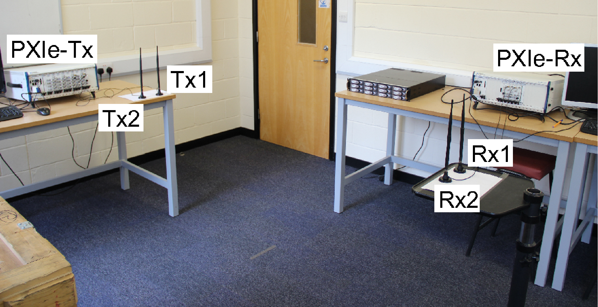
The physical layout of the experimental set-up is shown in Fig. 7 and the relative antenna spacing is provided in Fig. 8. In particular, the two transmit and two receive antennas are identical and are placed directly across from each other. As such, the channel between the transmitter and receiver has a strong LoS component. Therefore, the channel is assumed to be a Rician fading channel with a large -factor due to the short distance between the transmit and receive antennas, where is the ratio of the coherent power component, usually the LoS, to the non-coherent power components, usually NLoS. The omnidirectional transmit antennas broadcast on a frequency of GHz at Ms/s.


| (16) |
| (17) |
Channel measurements were collected to verify that the channel environment followed a Rician distribution. To achieve this, the transmitter broadcasts pulses at Ms/s on a carrier frequency of GHz at dBm peak power. Each pulse includes a frequency offset estimation section and a total of pulse samples are collected. A best fit approximation is then calculated for the collected data. In particular, a maximum likelihood estimation is fitted to the collected data. A Chi-squared goodness-of-fit test is then performed to ascertain that the distribution resulting from the maximum likelihood estimation fits at least of the data. The empirical CDF for each link is presented in Fig. 9. The results show that the channel does follow a Rician distribution with a factor that ranges between dB. The different -factors on the links between the transmit and receive antennas may be explained by the room geometry, the antenna positioning and the overall propagation environment. However, note that each of the CDFs has a different mean, which will be discussed in the next section.
III Equipment Constraints
Fig. 8 shows the physical layout of the experiment. Note that the cm inter–antenna separation used here is sufficient to guarantee very low, if any, spatial correlation when broadcasting at GHz with a m separation between the transmitter and receiver [42].
The physical environment through which the signal passes, starting from the SG–RF at the transmitter, until it reaches the –Bit Digitisers at the receiver, suffers from connector losses, differences in the RF chains, different phase responses, attenuations and similar. To study and model the effects of the hardware imperfections on the signal power:
- •
An RF coaxial cable with a dB attenuation is connected between each transmit and receive antenna.
- •
A pulse is transmitted at Ms/s on a carrier frequency of GHz at dBm peak power. Each pulse includes a frequency offset estimation section and a total of pulse samples were collected.
- •
The CDF for each of the fading coefficients is calculated and is shown in Fig. 10.
In an ideal environment, the means of the CDFs in Fig. 10 should be equal. However, imperfections in the hardware result in different means for each transmit to receiver antenna pair, as can be seen in Fig. 10. The differences between the channels can be modelled as a pim between the various link pairs in the channel matrix . Therefore, the channel coefficients are redefined as,
| (15) |
where is the channel attenuation coefficient from receive antenna to transmit antenna .
To locate the source of the discrepancy between the different channel attenuations, i.e., determine if the NI modules or the NI chassis is the source, the RF chains at the receiver were swapped around and the channels were estimated in configuration and configuration . To clarify, configuration represents the default modular set-up of the testbed while configuration refers to swapping the front-end modules around the transmit chassis. Fig. 10(a) shows the channel CDF for each transmit to receive antenna pair in configuration while Fig. 10(b) shows the channel CDF for each transmit to receive antenna pair in configuration . By considering the means of the CDFs in Figs. 10(a) and 10(b) and taking as a base, the various channel attenuations that result when the receiver is in configuration or in configuration are given in (16) and (17) respectively. Comparing Fig. 10(a) and Fig. 10(b), as well as the attenuations in (16) to those in (17), shows that they are very similar. Indeed, swapping of the RF chains has a minimal impact on the estimated mean of each channel attenuation. Thus, it can be assumed that the NI modules that compose the receive RF chains are the source of the hardware imperfections, and consequently lead to the differences in the means of the estimated CDFs. To account the hardware imperfections, the channel attenuation coefficients in (16) and (17) are taken into consideration in the derivation of the analytical model in Section IV. The accuracy of the derived analytical bound using the channel attenuation coefficients in (16) and (17) is demonstrated in Section VI where it is compared with empirical results.
IV Analytical Modeling
An analytical model for the aber performance of the experimental system is developed by considering the system model presented in Section II and the system constraints in Section III. The performance of SMlow and SMX over a single link in a noise-limited scenario is characterised by
| (18) |
where is the number of bits in error between the transmitted vector and , is the expectation across the channel , and is the conditional pep (pep) of deciding on given that is transmitted [43],
| (19) | |||||
where is half of the snr between the transmitter and receiver, and is the -function. As Fig. 8 indicates, the transmit and receive antennas in the experiment experience a very strong LoS environment. Accordingly, the channel between each transmit to receive antenna pair is characterised by Rician fading. A generic Rician channel is defined as
| (20) |
where is a complex normal, circular symmetric random variable with zero mean and unit variance. is the index of the transmit antenna and is the index of the receive antenna.
V Complexity Analysis
The computational complexity of the ml detector for SMlow (SMlow–ml) is compared to that of the ml detector for SMX (SMX–ml). The complexity is computed as the number of real multiplicative operations needed by each algorithm. The detailed derivation of each expression is considered in [13] and references therein.
- •
SMX–ml: The computational complexity of the SMX–ml receiver outlined in (13) is equal to,
(21) where is the spectral efficiency of the system. Note that in (13) requires complex multiplications.
- •
SMlow–ml: The computational complexity of the SMlow–ml receiver outlined in (14) is equal to,
(22) where the ml detector searches through the entire transmit and receive search spaces. Note that evaluating the Euclidean distance requires 2 complex multiplications, where each complex multiplication requires 4 real multiplications.
Considering (21) and (22), for the same spectral efficiency, the reduction in complexity of the SMlow–ml receiver relative to that of the SMX–ml receiver is given by,
| (23) |
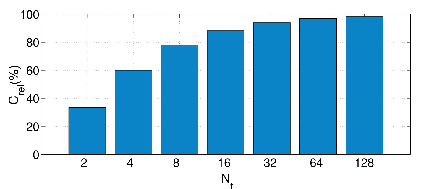
On the one hand, as can be seen in (22), the complexity of the SMlow receiver does not depend on the number of transmit antennas, and it is equal to the complexity of simo systems. On the other hand, the complexity of SMX increases linearly with the number of transmit antennas. Therefore, as the number of transmit antennas increases, the relative gain of the SMlow receiver increases. This can be seen in Fig. 11 where the relative complexity for is shown for both systems. In fact, Fig. 11 shows that for , SMlow offers a reduction in complexity, while a reduction in complexity can be seen for . The theoretical, simulation and empirical results for SMlow and SMX are now discussed.
VI Experimental Results and Numerical Analysis
VI-A Measurement Campaign
A stream of information bits is sent per transmission to obtain the experimental results. Two transmit antennas are available and BPSK (BPSK) is used for the signal constellation. As mentioned in Section II-A2, the real flat bandwidth is MHz. The information data is put in frames with bit each, as shown in the “Data section” of Fig. 5. The channel is estimated at the beginning and the end of every frame, resulting in channel estimations per transmission vector. The experiment is repeated times for every snr point. In addition, analytical and simulation aber curves are shown for SMlow in a Rician environment with and without the pims given in (16).
VI-B Results
The simulation, analytical and experimental results for the aber performance of SMlow in a LoS channel are illustrated in Fig. 12. In particular, the experimental results approximate the performance of the simulation results with pims and both the simulation, and experimental results, are closely approximated by the derived upper bound at a low aber.
This result serves to validate theoretical work done in the field where the presented snr along the x–axis is equivalent to the snr on . The large error between the experimental, simulation and analytical curves at high aber can be attributed to a number of factors including incorrect frequency offset estimation, timing recovery errors, synchronisation problems, poor channel estimation and decoding. Notably, incorrect frequency offset estimation can result in a systematic error contributing significantly to the % error seen at low snrs in the figure. As the snr increases, however, frequency offset estimation, timing recovery and channel estimation improve, leading to a lower aber as shown in Fig. 12. Differences between the measured and simulated aber curves can be attributed to channel imperfections such as channel correlations, mutual coupling and interference signals from the surrounding environment. Quantifying these imperfections is deemed important and requires channel modelling and interference measurement. However, addressing these effects is beyond the scope of this work and will be subject of future works.
SMlow performs best in a rich scattering environment where the channel between each transmit and receive antenna is unique. In particular, the larger the Euclidean distance between two received vectors is, the better the aber performance of SMlow becomes. Conversely, the more similar the channels are, the worse the aber of SMlow is. However, the channel uniqueness can be the result of the scattering environment or pims caused by hardware tolerances. The analytical and simulation results presented in Fig. 12 show the poor performance of SMlow in a Rician environment with no pim between the various transmitter to receiver links. Fig. 12 also shows the analytical and simulation aber for SMlow when pim are introduced. Indeed, the aber of SMlow improves significantly when these pims are introduced as each channel becomes more separable. This increases the Euclidean distance and improves performance.
If the channels between each transmit antenna to each receive antenna are similar, then the aber performance of SMlow degrades. This is seen when looking at the SMlow system without pims, illustrated by the dashed green line with triangular markers in Fig. 12. In fact, the aber of SMlow can be approximated by separating the error that originates from the estimation of the spatial constellation symbol and the error that originates from the estimation of the signal constellation symbol [44]. Therefore, depending on the environment, the main contributor to the overall aber of a SMlow system will be the erroneous detection of the spatial or signal constellation.

When pims are introduced, the Euclidean distance between the channel signatures increases. This decreases the error contribution of the spatial component of SMlow. Hence, when the snr is sufficiently high to have near perfect channel estimation, the error of the system is bound by the error from the signal component of SMlow. This separation can only be shown when iterative detection is used, which is proven to be sub-optimal [12]. In addition, work in [45] shows that the error when only the spatial constellation of SMlow is used for data transmission gets worse for an increasing factor in a Rician environment. This is the opposite to conventional modulation techniques since a larger factor for SMlow means a smaller Euclidean distance between the spatial constellation points which results in an increased aber performance. Indeed, it is the Euclidean distance between the different channels that determines the error in the spatial constellation detection. However, since ml–optimal detection is used at the receiver, separating the error from the spatial and signal symbols is strictly not permitted. Please note that the pims between the links are always obtained relative to the channel with the greatest attenuation, i.e., the values of the pim factors in (16) and (17) are always positive.

Furthermore, power imbalances between the transmitting antennas are shown to offer improved performance in terms of the aber when only the spatial constellation of SMlow is used, i.e., when ssk (ssk) is the underlying modulation technique. In particular, an optimised power allocation for a various number of transmit antennas is addressed in [23], where the authors show that there is optimal power allocation between the transmitting antennas which can serve to increases the Euclidean distance between the channel signatures and improve the aber performance of SMlow. Indeed, SMlow has also been successfully applied to an AWGN optical wireless channel where it is shown that pims greatly improve the aber performance [46].
The simulation, analytical and experimental results for the aber performance of SMX in a LoS channel are illustrated in Fig. 13. In particular, the experimental results closely follow the performance of the simulation results with pims and both the simulation, and experimental results, are closely approximated by the derived upper bound at low aber when the hardware imperfections are taken into account. This result serves to validate theoretical work done in the field. The results in Fig. 13 demonstrate that the SMX system, like the SMlow system, also benefits from the pims in the hardware. The SMX system exhibits approximately a coding gain when compared to SMlow at an aber of . This coding gain can also be seen at an aber of in Fig. 14, where the simulation and analytical results for the aber performance of SMlow and SMX are shown when there are no pims between the links.


The coding gain of SMX relative to SMlow is expected when there are few transmit antennas. The Euclidean distance between the transmit vectors, and therefore the variance in (19), in SMX is larger than in SMlow. However, the aim of this paper is to show that empirical results validate the simulation and analytical work done in the field, which can be seen in both Fig. 12 and Fig. 13. Unfortunately, due to the limited number of transmitter and receiver RF chains available, there are no experimental results for systems with a larger number of transmit or receive antennas where SMlow is shown to perform better than SMX. These empirical results will be the focus of future research. Nonetheless, the accuracy of the theoretical and simulation results of SMX and SMlow with a large number of transmit and receive antennas can be extrapolated from the presented results.
Fig. 15 compares the aber between SMlow (solid lines) and SMX (dashed lines) in a system with a large number of transmit antennas. Each system operates in a Rayleigh fading environment with a spectral efficiency of and four receive antennas. The results demonstrate the coding gains available to a SMlow system as compared to SMX when a large number of transmit antennas are available. In particular, SMlow with offers a coding gain of up to dB with respect to SMX with and a coding gain of dB with respect to SMX with . These performance gains stem from the greater Euclidean distance between the transmit vectors for SMlow. It is important to note that although SMlow is simulated as having transmit antennas available, it requires only a single RF chains, while SMX requires RF chains for the transmit antennas. Furthermore, to achieve the aber performance illustrated in Fig. 15, SMlow requires unique channels. In this work, a unique channel is assumed to be available only with the addition of a single transmit antenna. However, work in [6, 25] and others, look at creating multiple channel signatures without the need for a large number of physical transmit antennas while maintaining a similar aber performance to the traditional SMlow scheme.
This work demonstrates that the hardware tolerances of practical communication systems are beneficial for the aber performance of both SMlow and SMX. This behaviour along with the requirement for a single RF chain, make SMlow a viable candidate for future wireless networks.
VII Summary and Conclusion
In this work, the aber performance of SMlow and SMX has been validated experimentally for the first time. In particular, the encoding and decoding processes were presented. The experimental testbed, equipment and channel conditions were then described in detail and the aber of SMlow and SMX were obtained in a practical testbed environment. In addition, the experimental results were compared to both simulation and analytical approaches. As a result, it has been shown that a Rician channel with different channel attenuations closely described the behaviour of SMlow and SMX in the physical environment. Furthermore, it was demonstrated that the different channel attenuations resulted from various hardware imperfections at the transmitter and receiver RF chains. In fact, the induced power imbalances resulted in significant coding gains for the practical systems relative to the theoretical predictions without such power imbalances. To this extent, SMlow and SMX performed as expected relative to the theoretical work when the power imbalances were introduced in the analytical model. This result validated the SMlow principle. The performance gains exhibited by SMlow in the practical implementation make SMlow a viable candidate for future wireless networks and particularly for systems with a large number of transmit antennas available.
It is worth noting that the presented work may be extended in a number of different ways that would broaden its applicability. Empirical results that demonstrate the performance of SMlow and SMX with a large number of transmit and receive antennas remain to be obtained. In light of the above results, the aber performance of SMlow and SMX is expected to follow the theoretical models, but these results are essential to validate the aber performance for both SMlow and SMX systems. In addition, channel imperfections such as channel correlations and mutual antenna coupling along with the impact of interfering signals from neighbouring transmitters on the same frequency, should be analysed. Furthermore, obtaining empirical results for the capacity and energy efficiency of SMlow are of great interest for future research, particularly since SMlow is projected to have large energy efficiency gains when compared to other traditional mimolow schemes since it requires only a single RF chain. As a consequence, the quiescent power and circuit power can be kept at low levels. Acquiring the hardware which would enable the accurate measurement of these aspects is key. Lastly, the implementation of the SMlow detection algorithm on a DSP or an FPGA brings with it a number of optimisation challenges such as the use of multi-threading, pipeling, fixed point computations and others. The deployment of SMlow on an FPGA or a DSP has yet to be demonstrated.
It has been shown that SMlow is a simple, low cost, mimolow technique, which has now demonstrated excellent performance in a LoS wireless channel. Therefore, this work shows that SMlow is a promising practical approach to obtaining the enhanced performance of spatial multiplexing without introducing high processor complexity and high power consumption that would occur when using other spatial multiplexing approaches. The aim now is to investigate the performance of SMlow in a range of experimental channel conditions and further study its potential.
Acknowledgement
We gratefully acknowledge partial support by the University of Edinburgh Initiating Knowledge Transfer Fund (IKTF), EPSRC Fellowship (EP/K008757/1), RCUK (EP/G042713/1,UK-China Science Bridges ”R&D on (B)4G Wireless Mobile Communications”), the European Union (PITNGA2010264759, ”GREENET”), and the Key Laboratory of Cognitive Radio and Information Processing (Guilin University of Electronic Technology), Ministry of Education, China (Grant No.: 2013KF01).
References
- [1] E. Telatar, “Capacity of Multi-Antenna Gaussian Channels,” European Trans. on Telecommun., vol. 10, no. 6, pp. 585–595, Nov. / Dec. 1999.
- [2] J. Mietzner, R. Schober, L. Lampe, W. H. Gerstacker, and P. A. Höeher, “Multiple-Antenna Techniques for Wireless Communications - A Comprehensive Literature Survey,” IEEE Commun. Surveys Tutorials, vol. 11, no. 2, pp. 87 –105, 2009.
- [3] R. Mesleh, H. Haas, Y. Lee, and S. Yun, “Interchannel Interference Avoidance in MIMO Transmission by Exploiting Spatial Information,” in Proc. of the 16th IEEE Int. Symp. on Personal, Indoor and Mobile Radio Commun. (PIMRC), vol. 1, Berlin, Germany, 11-14 Sep. 2005, pp. 141–145.
- [4] R. Mesleh, H. Haas, S. Sinanović, C. W. Ahn, and S. Yun, “Spatial Modulation,” IEEE Trans. on Veh. Tech., vol. 57, no. 4, pp. 2228 – 2241, Jul. 2008.
- [5] N. Serafimovski, M. Di Renzo, S. Sinanović, R. Y. Mesleh, and H. Haas, “Fractional Bit Encoded Spatial Modulation (FBE–SM),” IEEE Commun. Lett., vol. 14, no. 5, pp. 429–431, May 2010.
- [6] A. Younis, N. Serafimovski, R. Mesleh, and H. Haas, “Generalised Spatial Modulation,” in Asilomar Conf. on Signals, Systems, and Computers, Pacific Grove, CA, USA, Nov. 2010.
- [7] J. Jeganathan, A. Ghrayeb, L. Szczecinski, and A. Ceron, “Space Shift Keying Modulation for MIMO Channels,” IEEE Trans. on Wireless Commun., vol. 8, no. 7, pp. 3692–3703, Jul. 2009.
- [8] G. Auer, V. Giannini, C. Desset, I. Godor, P. Skillermark, M. Olsson, M. Imran, D. Sabella, M. Gonzalez, O. Blume, and A. Fehske, “How Much Energy is Needed to Run a Wireless Network?” IEEE Wireless Commun., vol. 18, no. 5, pp. 40–49, 2011.
- [9] C. Desset, B. Debaillie, V. Giannini, A. Fehske, G. Auer, H. Holtkamp, W. Wajda, D. Sabella, F. Richter, M. J. Gonzalez, H. Klessig, I. Godor, M. Olsson, M. A. Imran, A. Ambrosy, and O. Blume, “Flexible Power Modeling of LTE Base Stations,” in IEEE Wireless Commun. and Networking Conf. (WCNC), Shanghai, China, Apr. 1–4 2012, pp. 2858 –2862.
- [10] A. Stavridis, S. Sinanović, M. D. Renzo., H. Haas, and P. Grant, “An Energy Saving Base Station Employing Spatial Modulation,” in IEEE 17th Int. Workshop on Computer Aided Modeling and Design of Commun. Links and Networks (CAMAD), Sep. 17–19 2012, pp. 231 –235.
- [11] A. Stavridis, S. Sinanović, M. D. Renzo, and H. Haas, “A Power Saving Dual-Hop Architecture Based on Hybrid Spatial Modulation,” in 2012 Conf. Record of the Forty Sixth Asilomar Conf. on Signals, Systems and Computers (ASILOMAR), Nov. 4–7 2012, pp. 1366–1370.
- [12] J. Jeganathan, A. Ghrayeb, and L. Szczecinski, “Spatial Modulation: Optimal Detection and Performance Analysis,” IEEE Commun. Lett., vol. 12, no. 8, pp. 545–547, 2008.
- [13] A. Younis, S. Sinanović, M. D. Renzo, R. Mesleh, and H. Haas, “Generalised Sphere Decoding for Spatial Modulation,” in IEEE Trans. on Commun., to appear. [Online]. Available: http://arxiv.org/abs/1305.1478
- [14] A. Younis, R. Mesleh, H. Haas, and P. M. Grant, “Reduced Complexity Sphere Decoder for Spatial Modulation Detection Receivers,” in 2010 IEEE Global Telecommun. Conf. (GLOBECOM), Miami, USA, Dec. 2010, pp. 1 –5.
- [15] A. Younis, M. Di Renzo, R. Mesleh, and H. Haas, “Sphere Decoding for Spatial Modulation,” in Proc. of IEEE Int. Conf. on Commun. (ICC), Kyoto, Japan, 5–9 Jun. 2011, pp. 1 –6.
- [16] R. Mesleh, M. Di Renzo, H. Haas, and P. M. Grant, “Trellis Coded Spatial Modulation,” IEEE Trans. on Wireless Commun., vol. 9, no. 7, pp. 2349–2361, Jul. 2010.
- [17] M. Di Renzo and H. Haas, “A General Framework for Performance Analysis of Space Shift Keying (SSK) Modulation for MISO Correlated Nakagami-m Fading Channels,” IEEE Trans. on Commun., vol. 58, no. 9, pp. 2590 –2603, Sep. 2010.
- [18] S. U. Hwang, S. Jeon, S. Lee, and J. Seo, “Soft-Output ML Detector for Spatial Modulation OFDM Systems,” IEICE Electronics Express, vol. 6, no. 19, pp. 1426�–1431, Oct. 2009.
- [19] M. Di Renzo and H. Haas, “Space Shift Keying (SSK) Modulation with Partial Channel State Information: Optimal Detector and Performance Analysis over Fading Channels,” IEEE Trans. on Commun., vol. 58, no. 11, pp. 3196 –3210, Nov. 2010.
- [20] S. S. Ikki and R. Mesleh, “A General Framework for Performance Analysis of Space Shift Keying (SSK) Modulation in the Presence of Gaussian Imperfect Estimations,” IEEE Commun. Lett., vol. 16, no. 2, pp. 228 –230, Feb. 2012.
- [21] E. Basar, U. Aygolu, E. Panayirci, and H. V. Poor, “Performance of Spatial Modulation in the Presence of Channel Estimation Errors,” IEEE Commun. Lett., vol. 16, no. 2, pp. 176 –179, Feb. 2012.
- [22] M. D. Renzo, D. D. Leonardis, F. Graziosi, and H. Haas, “Space Shift Keying (SSK) MIMO with Practical Channel Estimates,” IEEE Trans. on Commun., vol. 60, no. 4, pp. 998 –1012, Apr. 2012.
- [23] M. Di Renzo and H. Haas, “Improving the Performance of Space Shift Keying (SSK) Modulation via Opportunistic Power Allocation,” IEEE Commun. Lett., vol. 14, no. 6, pp. 500 –502, 2010.
- [24] T. Handte, A. Muller, and J. Speidel, “BER Analysis and Optimization of Generalized Spatial Modulation in Correlated Fading Channels,” in Veh. Tech. Conf. Fall (VTC Fall-2009), Anchorage, AK, Sep. 20–23 2009, pp. 1 –5.
- [25] E. Basar, U. Aygolu, E. Panayirci, and V. H. Poor, “Space-Time Block Coded Spatial Modulation,” IEEE Trans. on Commun., vol. 59, no. 3, pp. 823 –832, Mar. 2011.
- [26] M. Di Renzo and H. Haas, “On Transmit-Diversity for Spatial Modulation MIMO: Impact of Spatial-Constellation Diagram and Shaping Filters at the Transmitter,” in IEEE Trans. on Veh. Tech., 2013, to appear. Available: IEEE Xplore Early Access.
- [27] N. Serafimovski, S. Sinanovic, M. Di Renzo, and H. Haas, “Dual-hop Spatial Modulation (Dh-SM),” in Proc. of the IEEE Veh. Tech. Conf. (VTC Spring), Budapest, Hungary, May 15–18, 2011, pp. 1–5.
- [28] A. Stavridis, S. Sinanović, M. D. Renzo., and H. Haas, “Energy Evaluation of Spatial Modulation at a Multi-Antenna Base Station,” in Proc. of the 78th IEEE Veh. Tech. Conf. (VTC), Las Vegas, USA, Sep. 2–5, 2013.
- [29] M. Di Renzo and H. Haas, “Bit Error Probability of Spatial Modulation (SM) MIMO over Generalized Fading Channels,” IEEE Trans. on Veh. Tech., vol. 61, no. 3, pp. 1124 –1144, Mar. 2012.
- [30] A. Younis, W. Thompson, M. D. Renzo, C.-X. Wang, M. A. Beach, H. Haas, and P. M. Grant, “Performance of Spatial Modulation using Measured Real-World Channels,” in Proc. of the 78th IEEE Veh. Tech. Conf. (VTC), Las Vegas, USA, Sep. 2–5 2013. [Online]. Available: http://arxiv.org/abs/1305.3437
- [31] M. Di Renzo, H. Haas, and P. M. Grant, “Spatial Modulation for Multiple-Antenna Wireless Systems: A Survey,” IEEE Commun. Mag,, vol. 49, no. 11, pp. 182–191, Nov. 2011.
- [32] National Instruments, NI PXIe-5622 Specifications, 2011, 16-Bit IF Digitizer with Onboard Signal Processing.
- [33] P. Chambers, X. Hong, Z. Chen, C.-X. Wang, M. Beach, and H. Haas, “The UC4G Wireless MIMO Testbed,” in IEEE Global Commun. Conf. (GLOBECOM), Anaheim, USA, Dec. 3–7 2012, pp. 4368–4373.
- [34] G. J. Foschini, “Layered Space-Time Architecture for Wireless Communication in a Fading Environment when Using Multi-Element Antennas,” Bell Labs Tech. J., vol. 1, no. 2, pp. 41–59, 1996.
- [35] S. Tiiro, J. Ylioinas, M. Myllyla, and M. Juntti, “Implementation of the Least Squares Channel Estimation Algorithm for MIMO-OFDM Systems,” in Proc. of the International ITG Workshop on Smart Antennas (WSA 2009), Berlin, Germany, 16–18 Feb. 2009.
- [36] L. Lo Presti and M. Mondin, “Design of optimal FIR raised-cosine filters,” Electronics Lett., vol. 25, no. 7, pp. 467 –468, Mar. 1989.
- [37] J. L. Massey, “Optimum Frame Synchronization,” IEEE Transactions on Communications, vol. 20, pp. 115–119, 1972.
- [38] H. Xuefei and C. Jie, “Implementation Frame Synchronization for MIMO-OFDM System with ZCZ-codes,” in IEEE Int. Symp. on Microwave, Antenna, Propagation and EMC Tech. for Wireless Commun. (MAPE), vol. 1, Aug. 8–12 2005, pp. 241 – 244 Vol. 1.
- [39] J.-J. van de Beek, M. Sandell, M. Isaksson, and P. Ola Borjesson, “Low-complex Frame Synchronization in OFDM Systems,” in IEEE Int. Conf. on Universal Personal Commun., Tokyo, Japan, Nov. 6–10 1995, pp. 982 –986.
- [40] H. Hashemi, “The Indoor Radio Propagation Channel,” Proceedings of the IEEE, vol. 81, no. 7, pp. 943 –968, Jul. 1993.
- [41] D. McNamara, M. Beach, and P. Fletcher, “Experimental Investigation of the Temporal Variation of MIMO Channels,” in IEEE 54th Veh. Tech. Conf. (VTC 2010-Fall), vol. 2, Atlantic City, USA, Oct. 7–11 2001, pp. 1063 –1067 vol.2.
- [42] F. Quitin, C. Oestges, F. Horlin, and P. D. Doncker, “Multipolarized MIMO Channel Characteristics: Analytical Study and Experimental Results,” IEEE Trans. on Antennas and Propagation, vol. 57, no. 9, pp. 2739 –2745, 2009.
- [43] M. D. Renzo and H. Haas, “Performance analysis of Spatial Modulation,” in Int. ICST Conf. on Commun. and Networking in China (CHINACOM),, Aug. 2010, pp. 1 –7.
- [44] M. Di Renzo and H. Haas, “Bit Error Probability of Space Modulation over Nakagami-m Fading: Asymptotic Analysis,” IEEE Commun. Lett., vol. 15, no. 10, pp. 1026 –1028, Oct. 2011.
- [45] M. D. Renzo and H. Haas, “Space Shift Keying (SSK-) MIMO over Correlated Rician Fading Channels: Performance Analysis and a New Method for Transmit-Diversity,” in IEEE Trans. on Commun., vol. 59, no. 1, Jan. 2011, pp. 116–129.
- [46] T. Fath, H. Haas, Marco Di Renzo, and R. Mesleh, “Spatial Modulation Applied to Optical Wireless Communications in Indoor LOS Environments,” in IEEE Proc. of the Global Commun. Conf. (GLOBECOM), Houston, Texas, USA, 5–9 Dec. 2011, pp. 1–5, 5 pages.