Non-simple genus minimizers in lens spaces

Heegaard Floer homology, introduced by Ozsváth and Szabó [14], has been very successful in the study of low-dimensional topology. One important property of Heegaard Floer homology is that it detects Thurston norm of $3$–manifolds [16]. For a closed oriented $3$–manifold $Y$, its Thurston norm is always zero on the torsion subgroup of $H_{1}(Y;\mathbb{Z})$. However, there is another kind of “norm” function we can define on the torsion subgroup of $H_{1}(Y;\mathbb{Z})$. To define it, let us first recall the rational genus of a rationally null-homologous knot $K\subset Y$ defined by Calegari and Gordon [6].

Suppose that $K$ is a rationally null-homologous oriented knot in $Y$, and $\nu(K)$ is a tubular neighborhood of $K$. A properly embedded, oriented, connected surface $F\subset Y\backslash\overset{\circ}{\nu}(K)$ is called a rational Seifert surface for $K$ if $\partial F$ consists of coherently oriented parallel curves on $\partial\nu(K)$ and the orientation of $\partial F$ is coherent with the orientation of $K$. The rational genus of $K$ is defined to be

where $F$ runs over all the rational Seifert surfaces for $K$ and $\mu\subset\partial\nu(K)$ is the meridian of $K$.

The rational genus is a natural generalization of the genus of null-homologous knots. Moreover, given a torsion class in $H_{1}(Y)$, we can consider the minimal rational genus over all knots in this torsion class. More precisely, given $a\in\mathrm{Tors}H_{1}(Y)$, let

This function $\Theta$ was introduced by Turaev [24] in a slightly different form. Turaev regarded $\Theta$ as an analogue of Thurston norm [22], in the sense that it measures the minimal normalized Euler characteristic of a “folded surface” representing a given class in $H_{2}(Y;\mathbb{Q}/\mathbb{Z})$.

Recall that a rational homology $3$–sphere $Y$ is an L-space if $\mathrm{rank}\widehat{HF}(Y)=|H_{1}(Y;\mathbb{Z})|$. A rationally null-homologous knot $K$ in a $3$–manifold $Y$ is Floer simple if $\mathrm{rank}\widehat{HFK}(Y,K)=\mathrm{rank}\widehat{HF}(Y)$. In [12], it is shown that Floer simple knots in L-spaces have the smallest rational genus among all knots in the same homology class.

An important class of L-spaces is lens spaces. Hedden [8] and Rasmussen [18] observed that for any one-dimensional homology class in a lens space, there exists a knot in this homology class which is Floer simple. Let $U_{1}\cup U_{2}$ be a genus one Heegaard splitting of a lens space $L(p,q)$, and let $D_{1},D_{2}$ be meridian disks in $U_{1},U_{2}$ such that $\partial D_{1}\cap\partial D_{2}$ consists of exactly $p$ points. A knot in $L(p,q)$ is called simple if it is either the unknot or the union of two arcs $\gamma_{1}\subset D_{1}$ and $\gamma_{2}\subset D_{2}$. Up to isotopy there is exactly one simple knot in each homology class, and every simple knot is Floer simple. Hence simple knots in lens spaces are genus minimizers in their homology classes, which answers a question of Rasmussen [18] affirmatively.

Rasmussen [18] also asked whether simple knots are the unique genus minimizers in their homology classes, and if they are not, what the genus minimizers are. Baker [2] showed that if the rational genus of a knot in $L(p,q)$ is less than $\frac{1}{4}$, and the minimal rational Seifert surface has only one boundary component, then the knot is a one-bridge knot. In this paper, we answer Rasmussen’s question negatively in some cases, and in a very strong sense.

Baker gave an independent proof of Theorem 1.1 using the methods of [4] after learning about some of our examples [1].

Figure 1 displays the “simplest” non-simple genus minimizer we found. The knot $K_{0}$ is the $(1,2)$–cable of the $(1,2)$–torus knot in $L(8,1)$. The simple knot in this homology class is the $(1,4)$–torus knot. These two knots are not isotopic because their complements are not homeomorphic. The knot $K_{0}$ recurs throughout the various classes of examples that we study.

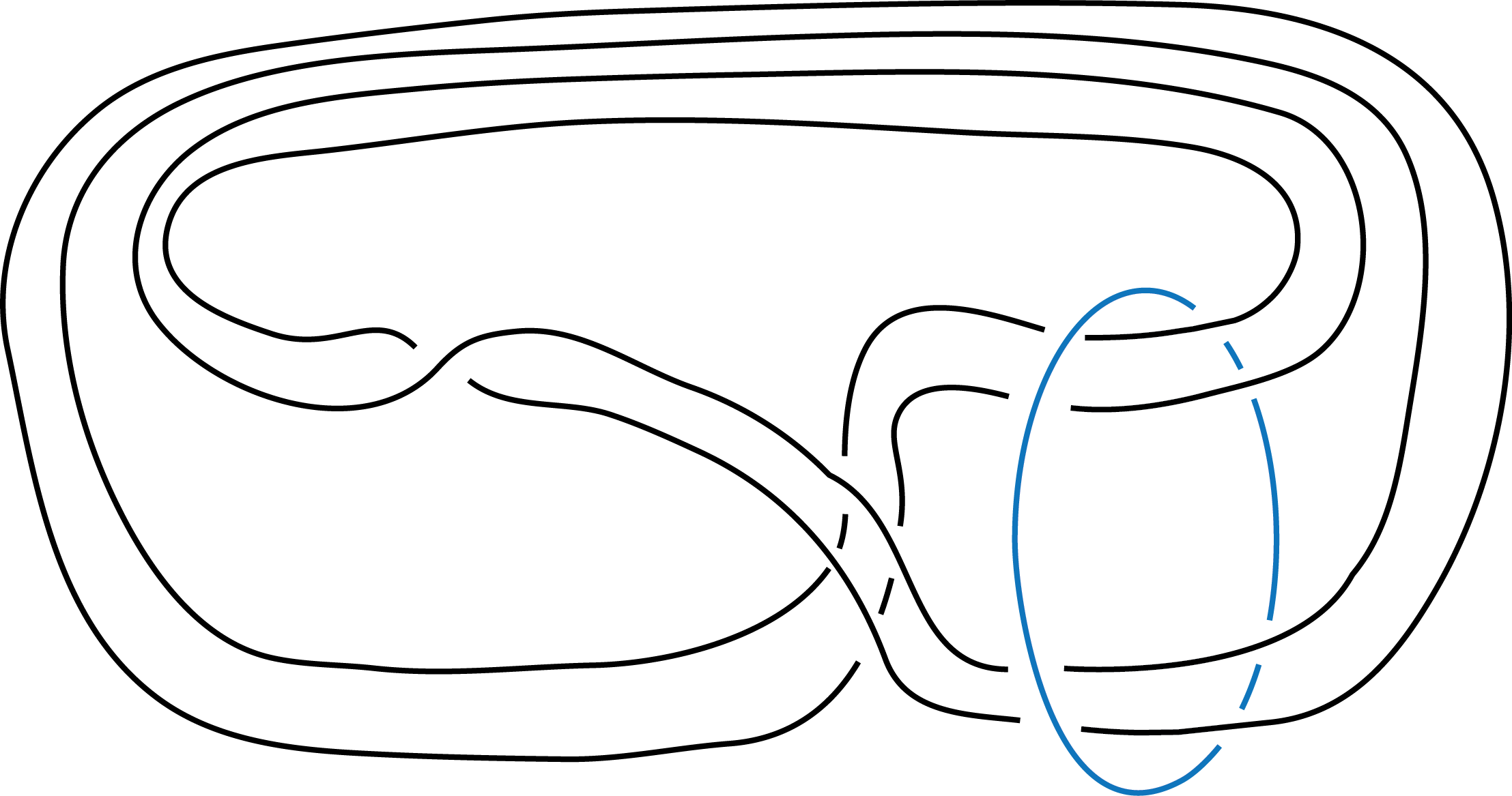
The examples we construct all have large rational genus, and they do not appear to be Floer simple knots. For instance, $K_{0}$ has rational genus $\frac{1}{2}$, and we confirmed that it is not Floer simple. It is possible that simple knots with small rational genus are the unique genus minimizers in their homology classes. For example, this could be the case for knots with rational genus less than $\frac{1}{2}$, which include the dual Berge knots [8, 18]. It is also possible that simple knots are the only Floer simple knots in lens spaces.

The lens space $L(2k,q)$ contains a (geometrically) incompressible closed surface $\Pi$, which is necessarily nonorientable. Rubinstein [19] proved that $\Pi$ is unique up to isotopy, and its genus $N(2k,q)$ can be computed by [5] (see also the end of Section 3). Recently, Johnson [10] proved that any nonorientable surface in $L(2k,q)$ with a given genus $\geq N(2k,q)$ is unique up to isotopy. Rubinstein’s result characterizes the genus-minimizing knots in the homology class $k\in H_{1}(L(2k,q))$.

The paper is organized as follows. In Section 2, we construct a family of non-simple rational genus minimizers via the cabling construction. In Section 3, we describe all the rational genus minimizers in order 2 homology classes. In Section 4, we get more examples (most of them hyperbolic) by stabilizing the example in Figure 1. In Section 5, we show that some order 2 homology classes contain infinitely many non-isotopic genus minimizers by using the annulus twist construction [13].

From now on we assume that $p>q\geq 1$ and $\gcd(p,q)=1$. We choose the following presentation for the lens space $L(p,q)$. Take a positive Hopf link $L_{1}\cup L_{2}\subset S^{3}$. $L(p,q)$ is obtained by $\frac{p}{q}$–surgery on $L_{2}$. Let $U_{1}$ be a tubular neighborhood of $L_{1}$, $T=\partial U_{1}$, and $U_{2}=\overline{L(p,q)-U_{1}}$. Thus, $U_{1}\cup_{T}U_{2}$ is the (unique) genus one Heegaard splitting of $L(p,q)$.

Let $[L_{1}]=1\in H_{1}(L(p,q))\cong\mathbb{Z}/p\mathbb{Z}$. Define

by requiring $q\varphi_{q}(a)\equiv a\pmod{p}$. Then the knot $K(p,q,a)$ represents the homology class $\varphi_{q}(a)$. In fact, if we push $K(p,q,a)$ into $U_{1}$, we get an index–$\varphi_{q}(a)$ closed braid in $U_{1}$.

In general, for any knot $K\subset U_{1}$, there is a canonical longitude of $K$ which is null-homologous in $S^{3}-\nu(K)\supset U_{1}-\nu(K)$. As usual in Dehn surgery, we parametrize the set of slopes on $K$ by $\mathbb{Q}\cup\{\infty\}$ so that the canonical longitude is $0$.

The following lemma is elementary.

The Thurston norm of a graph manifold is easily determined by the following lemma.

Suppose that $K\subset Y$ is a knot with a frame $\lambda$ and meridian $\mu$. Let $C\subset\partial\nu(K)$ be a simple closed curve which is homologous to $p[\mu]+q[\lambda]$. Then we say that $C$ is the $(p,q)$–cable of $K$ and denote it $C=C(p,q)\circ K$.

Let $\Pi_{h}$ denote the closed connected nonorientable surface of genus $h$. Note that $H_{1}(\Pi_{h})\cong\mathbb{Z}^{h-1}\oplus\mathbb{Z}_{2}$. The following lemma about the unique torsion class in $H_{1}(\Pi_{h})$ is elementary, and the proof is left to the reader.

When the homology class $a$ has order $2$, the function $\Theta$ is essentially the minimal genus of nonorientable connected surfaces in a given homology class.

We record the following construction for the unique incompressible surface $\Pi\subset L(2k,q)$, which has been independently noted by others [1, 20]. Let $S(2k,q)$ denote the two-bridge link with branched double-cover $L(2k,q)$. Put $S(2k,q)$ in alternating two-bridge position, let $D$ denote the disk bounded by one of the link components in the projection plane, and perturb the other component to meet $D$ transversely. Then the preimage of $D$ under the branched covering map $L(2k,q)\to S^{3}$ is the surface $\Pi$. It is straightforward to verify that the resulting surface $\Pi$ is non-orientable, and furthermore that its genus equals $N(2k,q)$ (for example, by using the formula for this value that appears in [5, Theorem 6.1]).

More examples of genus minimizers can be constructed by stabilizing the cable examples in Section 2. For simplicity, we only consider a special case.

We keep the notation from the first paragraph of Section 2. Let $K_{0}=C(1,2)\circ C(1,2)\circ L_{1}$ be a knot in $U_{1}$. Let $\gamma$ be a small unknot about the “bottom-left” crossing between $K_{0}$ and $L_{2}$, as in Figure 3. We orient $K_{0}$, $L_{2}$, and $\gamma$ so that the linking number between any two of them is positive. For any integer $k>0$, $(-\frac{1}{k})$–surgery on $\gamma$ transforms $K_{0}$ into the $k$-fold positive stabilization of the closed braid $K_{0}$, denoted $K_{k}$.

There is another way to view the link $K_{0}\cup L_{2}\cup\gamma$. On the left of Figure 4, we draw $K_{0}$ as a curve on a genus $4$ once-punctured non-orientable surface $\Pi_{4,1}\subset U_{1}$. On the right of Figure 4, an additional knot $\gamma\subset U_{1}$ is added to the picture of $K_{0}\cup L_{2}$. This $3$–component link is isotopic to the link in Figure 3.

Let $(\mu_{0},\lambda_{0}),(\mathcal{M},\mathcal{L}),(\mu_{\gamma},\lambda_{\gamma})$ be the meridian-longitude pairs on $K_{0},L_{2},\gamma$. Let

The knot $K_{0}\subset S^{3}$ is an unknot. Clearly, it bounds a disk $D_{0}$ which intersects $L_{2}$ exactly four times and intersects $\gamma$ exactly once. Let $F_{0}=D_{0}\cap M$. Then $\chi_{-}(F_{0})=4$. Moreover, under the map

we have

The knot $\gamma$ bounds a disk $D_{\gamma}$ which intersects each of $K_{0},L_{2}$ exactly once. Let $F_{\gamma}=D_{\gamma}\cap M$. Then $\chi_{-}(F_{\gamma})=1$ and

From Figure 4, we see that the knot $\gamma$ can be isotoped to intersect $\Pi_{4,1}$ exactly once. Let $F=\Pi_{4,1}\cap M$. Then $F$ is a genus one surface with four boundary components and $\chi_{-}(F)=4$. We have

Given relatively prime positive integers $p,q$ with $\frac{p}{q}\geq 2(k+4)$, consider the homology class

which can be represented by an embedded surface $F_{k}$ with

We have

The effect of the $(-\frac{1}{k})$–surgery on $\gamma$ is to perform $k$ postive twists along $D_{\gamma}$. Moreover, the slope $\frac{-kp+q(k+4)^{2}}{p}$ on $K_{0}$ becomes $\frac{q(k+4)^{2}}{p}$, and the slope $\frac{p-qk}{q}$ on $L_{2}$ becomes $\frac{p}{q}$. Hence if we also do $\frac{p-qk}{q}$–surgery on $L_{2}$, we get a knot $K_{k}\subset U_{1}\subset L(p,q)$ in the homology class $k+4$.

The surface $F_{k}$ has $k+4$ boundary components on $\partial\nu(L_{2})$ and $p-q(k+4)$ boundary components on $\partial\nu(\gamma)$. After capping off these boundary components, we get a rational Seifert surface $\widehat{F_{k}}$ for $K_{k}\subset L(p,q)$ with

and the winding number of $\partial\widehat{F_{k}}$ on $\nu(K_{k})$ is $p$.

On the other hand, similarly to (1), the torus knot $T(1,k+4)\subset L(p,q)$ has a rational Seifert surface which is a fiber of the fibration on $L(p,q)-T(1,k)$ with norm

and the winding number of its boundary on $\nu(T(1,k+4))$ is $p$. Moreover, by Lemma 2.3, $T(1,k+4)$ is a simple knot, so it is genus-minimizing. Hence $K_{k}$ is also genus-minimizing. This finishes the proof of the following proposition.

Using SnapPy [7], we check that $M$ is a hyperbolic manifold. By the hyperbolic Dehn surgery theorem [23], $K_{k}$ is a hyperbolic knot in $L(p,q)$ for a generic triple $(p,q,k)$. Therefore, $K_{k}$ is generally not isotopic to $T(1,k+4)$.

In this section, we establish the second statement in Theorem 1.1 by studying the knots that arise from torsion curves on the unique incompressible surface $\Pi\subset L(2k,1)$.

We begin by recalling Osoinach’s annulus twist construction [13]. Let $Y$ be a closed, oriented 3-manifold and $A\subset Y$ an embedded annulus with boundary $\partial A=\alpha_{0}\cup\alpha_{1}$. The boundary component $\alpha_{i}$ has a meridian $\mu_{i}\subset\partial\nu(\alpha_{i})$ and a parallel push-off $\lambda_{i}=\partial\nu(\alpha_{i})\cap A$, and we orient these curves so that $\mu_{i}\cdot\lambda_{i}=+1$. Osoinach observes that surgery on the link $\alpha_{0}\cup\alpha_{1}\subset Y$, with framing $\mu_{i}+\frac{(-1)^{i}}{n}\lambda_{i}$ on $\alpha_{i}$, results in a 3-manifold $Y_{n}$ homeomorphic to $Y$ for all $n\in{\mathbb{Z}}$. In fact, the homeomorphism $Y_{n}\cong Y$ can be taken to be the identity outside of a regular neighborhood of $A$. We refer to this homeomorphism as the result of doing $n$ twists along $A$.

Now suppose that $\Pi\subset Y$ is a closed, embedded surface and $\alpha\subset\Pi$ an embedded curve with an orientable (that is, annular) regular neighborhood $N\subset\Pi$. Then $N$ is co-orientable, and we can push $\alpha$ off of $N$ in the two normal directions to obtain a pair of oriented curves that cobound an annulus $A$ meeting $\Pi$ precisely in $\alpha$. We can therefore use $A$ to perform the annulus twist construction. An annular twist of $Y$ along $A$ takes $\Pi$ to itself, and restricting the homeomorphism to $\Pi$ has the effect of doing a Dehn twist along $\alpha$.

We apply this construction in the following way. Take a disk $D\subset S^{3}$ and attach $k=a+b+2$ positive half-twisted bands to its boundary, where $a,b\in{\mathbb{Z}}^{+}$. The result is a non-orientable surface $F\subset S^{3}$ such that $b_{1}(F)=k$, ${\partial}F$ is an unknot, and $F$ induces the framing $2k$ on ${\partial}F$. Choose a curve $\gamma\subset F$ that runs once across each half-twisted band and a curve $\alpha\subset F$ that runs once across each of two of the bands that are $a+1$ apart and zero times across every other band. Note that $\gamma$ is uniquely determined up to isotopy within $F$ and so is $\alpha$ once we fix the specific pair of bands that it crosses. We position $\alpha$ and $\gamma$ so that they intersect minimally; since $a,b\geq 1$, they meet in two points. See Figure 5.

References

- [1] K. Baker, private communication.
- [2] K. Baker, Small genus knots in lens spaces have small bridge number, Algebr. Geom. Topol., 6 (2006), 1519–1621.
- [3] K. Baker, J. E. Grigsby, M. Hedden, Grid diagrams for lens spaces and combinatorial knot Floer homology, Int. Math. Res. Not. IMRN 2008, no. 10, Art. ID rnm024, 39 pp.
- [4] K. Baker, C. Gordon, J. Luecke, Bridge number and integral Dehn surgery, preprint, available at arXiv:1303.7018.
- [5] G. E. Bredon, J. W. Wood, Non-orientable surfaces in orientable 3-manifolds, Invent. Math. 7 (1969), 83–110.
- [6] D. Calegari, C. Gordon, Knots with small rational genus, Comment. Math. Helv. 88 (2013), no. 1, 85–130.
- [7] M. Culler, N. M. Dunfield, and J. R. Weeks, SnapPy, a computer program for studying the geometry and topology of –manifolds, http://snappy.computop.org.
- [8] M. Hedden, On Floer homology and the Berge conjecture on knots admitting lens space surgeries, Trans. Amer. Math. Soc. 363 (2011), no. 2, 949–968.
- [9] W. Jaco, Lectures on three-manifold topology, CBMS Regional Conference Series in Mathematics, 43. American Mathematical Society, Providence, R.I., 1980. xii+251 pp.
- [10] J. Johnson, One-sided and two-sided Heegaard splittings, preprint, available at arXiv:1112.0471.
- [11] W. Neumann, D. Zagier, Volumes of hyperbolic three-manifolds, Topology 24 (1985), no. 3, 307–332.
- [12] Y. Ni, Z. Wu, Heegaard Floer correction terms and rational genus bounds, preprint, available at arXiv:1205.7053.
- [13] J. Osoinach, Manifolds obtained by surgery on an infinite number of knots in , Topology 45 (2006), 725–733.
- [14] P. Ozsváth, Z. Szabó, Holomorphic disks and topological invariants for closed three-manifolds, Ann. of Math. (2), 159 (2004), no. 3, 1027–1158.
- [15] P. Ozsváth, Z. Szabó, Holomorphic disks and knot invariants, Adv. Math. 186 (2004), no. 1, 58–116.
- [16] P Ozsváth, Z Szabó, Holomorphic disks and genus bounds, Geom. Topol. 8 (2004), 311–334.
- [17] J. Rasmussen, Floer homology and knot complements, PhD Thesis, Harvard University (2003), available at arXiv:math.GT/0306378.
- [18] J. Rasmussen, Lens space surgeries and L-space homology spheres, preprint (2007), available at arXiv:0710.2531.
- [19] J. H. Rubinstein, One-sided Heegaard splittings of 3-manifolds, Pacific J. Math. 76 (1978), no. 1, 185–200.
- [20] J. H. Rubinstein, private communication.
- [21] M. Scharlemann, The complex of curves on non-orientable surfaces, J. London Math. Soc. (2), 25 (1982), 171–184.
- [22] W. Thurston, A norm for the homology of –manifolds, Mem. Amer. Math. Soc. 59 (1986), no. 339, i–vi and 99–130.
- [23] W. Thurston, The geometry and topology of three-manifolds, Princeton lecture notes (1980).
- [24] V. Turaev, A function on the homology of –manifolds, Algebr. Geom. Topol. 7 (2007), 135–156.