Limiting the Neighborhood: De-Small-World Network for Outbreak Prevention
Abstract
In this work, we study a basic and practically important strategy to help prevent and/or delay an outbreak in the context of network: limiting the contact between individuals. In this paper, we introduce the average neighborhood size as a new measure for the degree of being small-world and utilize it to formally define the de-small-world network problem. We also prove the NP-hardness of the general reachable pair cut problem and propose a greedy edge betweenness based approach as the benchmark in selecting the candidate edges for solving our problem. Furthermore, we transform the de-small-world network problem as an OR-AND Boolean function maximization problem, which is also an NP-hardness problem. In addition, we develop a numerical relaxation approach to solve the Boolean function maximization and the de-small-world problem. Also, we introduce the short-betweenness, which measures the edge importance in terms of all short paths with distance no greater than a certain threshold, and utilize it to speed up our numerical relaxation approach. The experimental evaluation demonstrates the effectiveness and efficiency of our approaches.
1 Introduction
The interconnected network structure has been recognized to play a pivotal role in many complex systems, ranging from natural (cellular system), to man-made (Internet), to the social and economical systems. Many of these networks exhibit the “small-world” phenomenon, i.e., any two vertices in the network is often connected by a small number of intermediate vertices (the shortest-path distance is small). The small-world phenomenon in the real populations was first discovered by Milgram [13]. In his study, the average distance between two Americans is around . Several recent studies [11, 14, 8] offer significant evidence to support similar observations in the online social networks and Internet itself. In addition, the power-law degree distribution (or scale-free property) which many of these networks also directly lead to the small average distance [1]. Clearly, the small-world property can help facilitate the communication and speed up the diffusion process and information spreading in a large network.
However, the small-world effect can be a dangerous double-edged sword. When a system is benefited from the efficient communication and fast information diffusion, it also makes itself more vulnerable to various attacks: diseases, (computer) virus, spams, and misinformation, etc. For instance, it has been shown that a small-world graph can have much faster disease propagation than a regular lattice or a random graph [15]. Indeed, the six degrees of separation may suggest that a highly infectious disease could spread to all six billion people living in the earth about size incubation periods of the diseases [15]. The small-word property of Internet and WWW not only enables the computer virus and spams to be much easier to spread, but also makes them hard to stop. More recently, the misinformation problem in the social networks has made several public outcry [3]. These small-world online social network potentially facilitate the spread of misinformation to reach a large number of audience in short time, which may cause public panic and have other disruptive effects.
To prevent an outbreak, the most basic strategy is to remove the affected individuals (or computers) from the network system, like quarantine. However, in many situations, the explicit quarantine may be hard to achieve: the contagious individuals are either unknown or hard to detect; or it is often impossible to detect and remove each infected individual; or there are many already being affected and it become too costly to remove all of them in a timely fashion. Thus, it is important to consider alternative strategies to help prevent and even delay the spreading where the latter can be essential in discovering and/or deploying new methods for dealing with the outbreaks.
Recently, there have been a lot of interests in understanding the network factors (such as the small-word and scale-free properties) in the epidemics and information diffusion process, and utilizing the network structures in detecting/preventing the outbreaks. Several studies have focused on modeling the disease epidemics on the small-world and/or scale-free networks [17, 15], [16]; in [12], Leskovec et al. study how to deploy sensors cost-effectively in a network system (sensors are assigned to vertices) to detect an outbreak; in [3], Budak et al. consider how to limit the misinformation by identifying a set of individuals that are needed to adopt the “good” information (being immune in epidemics) in order to minimize those being affected by the “bad” information (being infected in epidemics). In addition, we note that from a different angle (viral marketing), there have been a list of studies on the influence maximization problem [18, 9], which aim to discover a set of most influential seeds to maximize the information spreading in the network. From the disease epidemics perspective, those seeds (assuming being selected using contagious model) may need particular protection to prevent an outbreak.
In this work, we study another basic and practically important strategy to help prevent and/or delay an outbreak in the context of network: limiting the contact between individuals. Different from the pure quarantine approach, here individuals can still perform in the network system, though some contact relationships are forbidden. In other words, instead of removing vertices (individuals) form a network as in the quarantine approach, this strategy focuses on removing edges so that the (potential) outbreaks can be slowed down. Intuitively, if an individual contacts less number of other individuals, the chance for him or her to spread or being infected from the disease (misinformation) becomes less. From the network viewpoint, the edge-removal strategy essentially make the underlying (social) network less small-world, or simply “de-small-world”, i.e., the distances between individuals increase to delay the spreading process. In many situations, such a strategy is often easily and even voluntarily adopted. For instance, during the SARS epidemic in Beijing, 2004, there are much less people appearing in the public places. In addition, this approach can also be deployed in complement to the quarantine approach.
1.1 Our Contribution
Even though the edge-removal or de-small-world approach seems to be conceptually easy to understand, its mathematical foundation is still lack of study. Clearly, different edges (interactions) in the network are not being equivalent in terms of slowing down any potential outbreak: for a given individual, a link to an individual of high degree connection can be more dangerous than a link to another one with low degree connection. The edge importance (in terms of distance) especially coincides with Kleighnberg’s theoretical model [10] which utilizes the long-range edges on top of an underlying grid for explaining the small-world phenomenon. In this model, the long-range edges are the main factors which help connect the otherwise long-distance pairs with a smaller number of edges. However, there are no direct studies in fitting such a model to the real world graph to discover those long-range edges. In the mean time, additional constraint, such as the number of edges can be removed from the network, may exist because removing an edge can associate with certain cost. These factors and requirements give arise to the following fundamental research problem: how can we maximally de-small-world a graph (making a graph to be less small-world) by removing a fixed number of edges?
To tackle the de-small-world network problem, we make the following contributions in this work:
- 1.
We introduce the average neighborhood size as a new measure for the degree of being small-world and utilizes it to formally define the de-small-world network problem. Note that the typical average distance for measuring the small-world effects cannot uniformly treat the connected and disconnected networks; neither does it fit well with the spreading process. We also reformulate the de-small-world as the local-reachable pair cut problem.
- 2.
We prove the NP-hardness of the general reachable pair cut problem and propose a greedy edge betweenness based approach as the benchmark in selecting the candidate edges for solving the de-small-world network. We transform the de-small-world network problem and express it as a OR-AND Boolean function maximization problem, which is also an NP-hard problem.
- 3.
We develop a numerical relaxation approach to solve the de-small-world problem using its OR-AND boolean format. Our approach can find a local minimum based on the iterative gradient optimization procedure. In addition, we further generalize the betweenness measure and introduces the short betweenness, which measures the edge importance in terms of all the paths with distance no greater than a certain threshold. Using this measure, we can speed up the numerical relaxation approach by selecting a small set of candidate edges for removal.
- 4.
We perform a detailed experimental evaluation, which demonstrates the effectiveness and efficiency of proposed approaches.
2 Problem Definition and Preliminary
In this section, we first formally define the de-small-world network problem and prove its NP-hardness in (Subsection 2.1); then we introduce the basic greedy approaches based on edge betweenness which will serve as the basic benchmark (Subsection 2.2); and finally we show the de-small-world network problem can be transformed and expressed as a OR-AND Boolean function maximization problem (Subsection 2.3).
2.1 Problem Formulation
In order to model the edge-removal process and formally define the de-small-world network problem, a criterion is needed to precisely capture the degree of being small-world. Note that here the goal is to help prevent and/or delay the potential outbreak and epidemic process. The typical measure of small-world network is based on the average distance (the average length of the shortest path between any pair of vertices in the entire network). However, this measure is not able to provide unified treatment of the connected and cut network. Specifically, assuming a connected network is broken into several cut network and the average distance on the cut network is not easy to express. On the other hand, we note that the de-small-world network graph problem is different from the network decomposition (clustering) problem which tries to break the entire network into several components (connected subgraphs). From the outbreak prevention and delaying perspective, the cost of network decomposition is not only too high, but also may not be effective. This is because each individual component itself may still be small-world; and the likelihood of completely separating the contagious/infected group from the rest of populations (the other components) is often impossible.
Given this, we introduce the average neighborhood size as a new measure for the degree of being small-world and utilize it to formally define the de-small-world network problem. Especially, the new measure can not only uniformly treat both connected and cut networks and aims to directly help model the spreading/diffusion process. Simply speaking, for each vertex in a network where is the vertex set and is the edge set, we define the neighborhood of as the number of vertices with distance no greater than to , denoted as . Here is the user-specified spreading (or delaying) parameter which aims to measure the outbreak speed, i.e., in a specified time unit, the maximum distance between individual (source) to another one (destination) who can be infected if is infected. Thus, the average neighborhood size of , , can be used to measure the robustness of the network with respect to a potential outbreak in a certain time framework. Clearly, a potential problem of the small-world network is that even for a small , the average neighborhood size can be still rather large, indicating a large (expected) number of individuals can be quickly affected (within time framework ) during an outbreak process.
Formally, the de-small-world network problem is defined as follows:
Definition 1
(De-Small-World Network Problem) Given the edge-removal budget and the spreading parameter we seek a subset of edges , where , such that the average neighborhood size is minimized:
| (1) |
where is the neighborhood size of in the graph after removing all edges in from the edge set .
Note that in the above definition, we assume each vertex has the equal probability to be the source of infection. In the general setting, we may consider to associate each vertex with a probability to indicate its likelihood to be (initially) infected. Furthermore, we may assign each edge with a weight to indicate the cost to removing such an edge. For simplicity, we do not study those extensions in this work; though our approaches can be in general extended to handle those additional parameters. In addition, we note that in our problem, we require the spreading parameter . This is because for , this problem is trivial: the average neighborhood size is equivalent to the average vertex degree; and removing any edge has the same effect. In other words, when , the neighborhood criterion does not capture the spreading or cascading effects of the small-world graph. Therefore, we focus on , though in general is still relatively small (for instance, no higher than or in general).
Reachable Pair Cut Formulation: We note the de-small-world network problem can be defined in terms of the reachable pair cut formulation. Let a pair of two vertices whose distance is no greater than is referred to as a local-reachable pair or simply reachable pair. Let record the set of all local reachable pairs in .
Definition 2
(Reachable Pair Cut Problem) For a given local , if in , but , where is an edge set in , then we say is being local cut (or simply cut) by . Given the edge-removal budget and the spreading parameter , the reachable pair cut problem aims to find the edge set , such that the maximum number of pairs in is cut by .
Note that here the (local) cut for a pair of vertices simply refers to increase their distance; not necessarily completely disconnect them in the graph (). Also, since , i.e., every local-reachable pair in the remaining network is also the local-reachable in the original graph , the problem is equivalently to maximize and minimize the number of local reachable pairs . Finally, the correctness of such a reformulation (de-small-world problem=reachable pair cut problem) follows this simple observation: (and ). Basically, every reachable pair is counted twice in the neighborhood size criterion.
In the following, we study the hardness of the general reachable pair cut problem.
Theorem 1
Given a set of local reachable pairs in with respect to , the problem of finding edges () in such that the maximal number of pairs in being cut by is NP-Hard.
Note that in the general problem, can be any subset of . The NP-hardness of the general reachable pair cut problem a strong indicator that the de-small-world network problem is also hard. The proof of Theorem 1 is in Appendix. In addition, we note that the submodularity property plays an important role in solving vertex-centered maximal influence [9], outbreak detection [12], and limiting misinformation spreading [3] problems. However, such property does not hold for the edge-centered de-small-world problem.
Lemma 1
Let set function records the number of local reachable pairs in is cut by an edge set in graph . Function is neither submodular (diminishing return) nor supermodular.
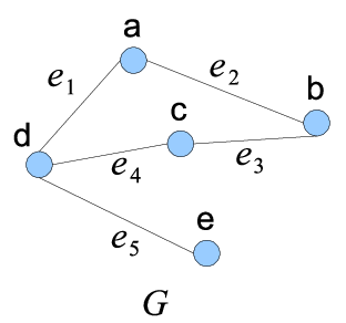
Proof Sketch: For a supermodular function: we have ; for a submodular function: we need show . Here we use two counter examples (suppose ). For in Figure 1, we can see that edge sets and cut (cut) respectively two reachable pairs and . Then we have ; however, . Therefore, supermodularity does not hold. For in Figure 1, we can see that edge set and each can only cut one reachable pair. However, could cut four pairs. That means, . Therefore, submodularity can not hold.

2.2 Greedy Betweenness-Based Approach
Finding the optimal solution for the de-small-world problem is likely to be NP-hard. Clearly, it is computationally prohibitive to enumerate all the possible removal edge set and to measure how many reachable pairs could be cut or how much the average neighborhood size is reduced. In the following, we describe a greedy approach to heuristically discover a solution edge-set. This approach also serves as the benchmark for the de-small-world problem.
The basic approach is based on the edge-betweenness, which is a useful criterion to measure the edge importance in a network. Intuitively, the edge-betweenness measures the edge important with respect to the shortest paths in the network. The high betweenness suggests that the edge is involved into many shortest paths; and thus removing them will likely increase the distance of those pairs linked by these shortest paths. Here, we consider two variants of edge-betweenness: the (global) edge-betweenness [5] and the local edge-betweenness [6]. The global edge-betweenness is the original one [5] and is defined as follows:
where is the total number of shortest paths between vertex and , and the total number of shortest paths between and containing edge .
The local edge-betweenness considers only those vertex pairs whose shortest paths are no greater than , and is defined as
The reason to use the local edge-betweenness measure is because in the de-small-world (and reachable pair cut) problem, we focus on those local reachable pairs (distance no greater than ). Thus, the contribution to the (global) betweenness from those pairs with distance greater than can be omitted. The exact edge-betweenness can be computed in worst case time complexity [2] where (the number of vertices) and (the number of edges) in a given graph, though in practical the local one can be computed much faster.
Using the edge-betweenness measure, we may consider the following generic procedure to select the edges for :
1) Select the top edges into , and remove those edges from the input graph ;
2) Recompute the betweenness for all remaining edges in the updated graph ;
3) Repeat the above procedure times until all edges are selected.
Note that the special case , where we select each edge in each iteration, the procedure is very similar to the Girvan-Newman algorithm [5] in which they utilize the edge-betweenness for community discovery. Gregory [6] generalizes it to use the local-edge betweenness. Here, we only consider to pickup edges and allow users to select the frequency to recompute the edge-betweenness (mainly for efficiency consideration). The overall time complexity of the betweenness based approach is (assuming the exact betweenness computation is adopted).
2.3 OR-AND Boolean Function and its Maximization Problem
In the following, we transform the de-small-world network problem and express it as a OR-AND Boolean function maximization problem, which forms the basis for our optimization problem in next section. First, we will utilize the OR-AND graph to help represent the de-small-world (reachable pair cut) problem. Let us denote the set of all the short paths in that have length at most .

OR-AND Graph: Given a graph , the vertex set of an OR-AND graph is comprised of three kinds of nodes , and , where each node in corresponds to a unique edge in , each node in corresponds to a short path in , and each node in corresponds to a unique reachable pair in (with respect to ). Figure 2(b) shows those nodes for graph in Figure 2(a). The edge set consists of two types of edges: 1) Each short path node in is linked with the vertices in corresponding to those edges in in the path. For instance path node in links to edge node and in in Figure 2(b). Each reachable pair node in links to those path nodes which connects the reachable pair . For instance, the reachable pair is connected with path node and in Figure 2(b).
Intuitively, in the OR-AND graph, we can see that in order to cut a reachable pair, we have to cut all the short paths between them (AND). To cut one short path, we need to remove only one edge in that path (OR). Let consists all the (simple) short paths between and whose length are no more than . For each short path in , let corresponds to a Boolean variable for edge : if , then the edge is not cut; if , then the edge is cut (). Thus, for each reachable pair , we can utilize the a Boolean OR-AND expression to describe it:
| (2) |
For instance, in the graph (Figure 2(b)),
Here, indicating the pair is being cut only if for both and are cut. For instance, if and , then ; and , but and , . Given this, the de-small-world problem (and the reachable pair cut problem) can be expressed as the following Boolean function maximization problem.
Definition 3
(Boolean Function Maximization Problem) Given a list of Boolean functions (such as , where ), we seek a Boolean variable assignment where exactly variables are assigned false ( iff , and ), such that the maximal number of Boolean functions being false ( corresponding to is cut by ).
Unfortunately, the Boolean function maximization problem is also NP-hard since it can directly express the general reachable pair cut problem. In the next section, we will introduce a numerical relation approach to solve this problem.
3 Path Algebra and Optimization Algorithm
In this section, we introduce a numerical relaxation approach to solve the Boolean function maximization problem (and thus the de-small-world problem). Here, the basic idea is that since the direct solution for the Boolean function maximization problem is hard, instead of working on the Boolean (binary) edge variable, we relax to it to be a numerical value. However, the challenge is that we need to define the numerical function optimization problem such that it meet the following two criteria: 1) it is rather accurately match the Boolean function maximization; and 2) it can enable numerical solvers to be applied to optimize the numerical function. In Subsection 3.1, we introduce the numerical optimization problem based on the path algebra. In Subsection 3.2, we discuss the optimization approach for solving this problem.
3.1 Path-Algebra and Numerical Optimization Problem
To construct a numerical optimization problem for the Boolean function maximization format of the de-small-world problem, we introduce the following path-algebra to describe all the short paths between any reachable pair in . For each edge in the graph , we associate it with a variable . Then, for any reachable pair , we define its corresponding path-algebra expression as follows:
| (3) |
Taking the path-algebra for in Figure 2 and Figure 3 as example, we have

Basically, the path-algebra expression directly corresponds to the Boolean expression by replacing with product (), with sum (), and Boolean variable with algebraic variable . Intuitively, records the weighted sum of each path in , where the weight is the product based on the edge variable . Note that when for every edge , when simply records the number of different short paths (with length no more than ) between and , i.e., . Furthermore, if assuming , then is equivalent to in each path , there is at least one edge variable is equivalent to . In other words, assuming if variable iff , then iff and iff .
Given this, we may be tempted to optimize the follow objective function based on the path-algebra expression to represent the Boolean function maximization problem:
.
However, this does not accurately reflect our goal, as to minimize , we may not need any (which shall be our main goal).
This is because corresponds to the weighted sum of path products.
Can we use the path-algebra to address the importance of in the objective function?
We provide a positive answer to this problem by utilizing an exponential function transformation. Specifically, we introduce the following numerical maximization problem based on the path expression:
| (4) |
Note that (each ), and only when , (the largest value for each term). When , the term can be rather small (approach ). The parameter is the adjusting parameter to help control the exponential curve and smooth the objective function. Furthermore, the summation constraint is to express the budget condition that there shall have variables with . Here is the total number of variables in the objective function ( if we consider every single edge variable ).
3.2 Gradient Optimization
Clearly, it is very hard to find the exact (or closed form) solution for maximizing function in Equation 4 under these linear constraints. In this section, we utilize the standard gradient (ascent) approach together with the active set method [7] to discover a local maximum. The gradient ascent takes steps proportional to the positive of the gradient iteratively to approach a local minimum. The active set approach is a standard approach in optimization which deals with the feasible regions (represented as constraints). Here we utilize it to handle the constraint in Equation 4.
Gradient Computation: To perform gradient ascent optimization, we need compute the gradient for each variable . Fortunately, we can derive a closed form of in as follows:
where is the sum of the path-product on all the paths going through and we treat in the path-product. More precisely, let be the set of all short paths (with length no more than ) between and going through edge , and then,
| (5) |
Using the example in Figure 2 and Figure 3, we have
Note that once we have all the gradients for each edge variable , then we update them accordingly,
where is the step size (a very small positive real value) to control the rate of convergence.
and Computation To compute the gradient, we need compute all and for . Especially, the difficulty is that even compute the total number of simple short paths (with length no more than ) between and , denoted as is known to be expensive. In the following, we describe an efficient procedure to compute and efficiently. The basic idea is that we perform a DFS from each vertex with traversal depth no more than . During the traversal form vertex , we maintain the partial sum of both and for each and where can reach within steps. After each traversal, we can then compute the exact value of and .
The DFS procedure starting from to compute all and is illustrated in Algorithm 1. In Algorithm 1, we maintain the current path (based on the DFS traversal procedure) in and its corresponding product is maintained in variable (Line and ). Then, we incrementally update assuming is the end of the path (Line ). In addition, we go over each edge in the current path, and incrementally update (, Line .) Note that we need invoke this procedure for every vertex to compute all and . Thus, the overall time complexity can be written as for a random graph where is the average vertex degree.
Overall Gradient Algorithm
The overall gradient optimization algorithm is depicted in Algorithm 2. Here, we use to describe all the edges which need be processed for optimization. At this point, we consider all the edges and thus . Later, we will consider to first select some candidate edges. The entire algorithm performs iteratively and each iteration has three major steps:
Step 1 (Lines ): it calculates the gradient of for every edge variable and an average gradient ;
Step 2 (Lines ): only those variables are not in the active set will be updated. Specifically, if the condition () is not met, we try to adjust back to the feasible region. Note that by using (Line ) instead of (Line ), we are able to increase the value of those whose gradient is below average. However, such adjustment can still guarantee the overall objective function is not decreased (thus will converge). Also, we make sure will be between and .
Step 3 (Lines ): the active set is updated. When an edge variable reaches or , we put them in the active set so that we will not need to update them in Step 2. However, for those edges variables in the active set, if their gradients are less (higher) than the average gradient for (), we will release them from the active set and let them to be further updated.
Note that the gradient ascent with the active set method guarantees the convergence of the algorithm (mainly because the overall objective function is not decreased). However, we note that in Algorithm 2, the bounded condition () may not be necessarily satisfied even with the update in Line . Though this can be achieved through additional adjustment, we do not consider them mainly due to the goal here is not to find the exact optimization, but mainly on identifying the smallest edges based on . Finally, the overall time complexity of the optimization algorithm is , given is the maximum number of iterations before convergence.
4 Short Betweenness and Speedup Techniques
In Section 3, we reformulate our problem into a numerical optimization problem. We further develop an iterative gradient algorithm to select the top edges in to . However, the basic algorithm can not scale well to very large graphs due to the large number () of variables involved. In this section, we introduce a new variant of the edge-betweenness and use it to quickly reduce the variables needed in the optimization algorithm (Algorithm 2). In addition, we can further speedup the DFS procedure to compute and in Algorithm 1.
4.1 Short Betweenness
In this subsection, we consider the following question: What edge importance measure can directly correlate with in the objective function in Eq. 4 so that we can use it to help quickly identify a candidate edge set for the numerical optimization described in Algorithm 2? In this work, we propose a new edge-betweenness measure, referred to as the short betweenness to address the this question. It is intuitively simple and has an interestingly relationship with respect to the gradient for each edge variable. It can even be directly applied for selecting using the generic procedure in Section 2 and is much more effective compared with the global and local edge-betweenness which measure the edge importance in terms of the shortest path (See comparison in Section 5).
Here we formally define as short betweenness.
Definition 4
(Short Betweenness:) The short betweenness for edge is as follows, .
Recall that means ; is the number of short paths between and ; and is the number of short paths between and which must go through edge . The following lemma highlights the relationship between the short betweenness and the gradient of edge variable :
Lemma 2
Assuming for all edge variables , then .
Proof Sketch:
Basically, when for every edge variable (this is also the initialization of Algorithm 2), the (negative) short betweenness serves a lower bound of the gradient . Especially, since the gradient is negative, the higher the gradient of is, the more likely it can maximize the objective function (cut more reachable pairs in . Here, the short betweenness thus provide an upper bound (or approximation) on (assuming all other edges are presented in the graph); and measures the the edge potential in removing those local reachable pairs. Finally, we note that Algorithm 1 can be utilized to compute and , and thus the short betweenness (just assuming for all edge variables).
Scaling Optimization using Short Betweenness: First, we can directly utilize the short betweenness to help us pickup a candidate set of edge variables, and then Algorithm 2 only need to work on these edge variables (considering other edge variables are set as ). Basically, we can choose a subset of edges which has the highest short betweenness in the entire graph. The size of has to be larger than ; in general, we can assume , where . In the experimental evaluation (Section 5), we found when , the performance of using candidate set is almost as good as the original algorithm which uses the entire edge variables. Once the candidate set edge set is selected, we make the following simple observation:
Lemma 3
Given a candidate edge set , if any reachable pair can be cut by where and , then, each path in must contains at least one edge in .
Clearly, if there is one path in does not contain an edge in , it will always linked no matter how we select and thus cannot cut by . In other words, has to be cut by if it can be cut by . Given this, we introduce . Note that can be easily computed by the DFS traversal procedure similar to Algorithm 1. Thus, we can focus on optimizing
| (6) |
Furthermore, let , which records those edges appearing in certain path linking a reachable pair cut by . Clearly, for those edges in , we can simply prune them from the original graph without affecting the final results. To sum, the short betweenness measure can help speed up the numerical optimization process by reducing the number of edge variables and pruning non-essential edges from the original graph.
5 Experimental Study
In this section, we report the results of the empirical study of our methods. Specifically, we are interested in the performance (in terms of reachable pair cut) and the efficiency (running time).
| Dataset | |||
|---|---|---|---|
| Gnutella04 | 10,876 | 39,994 | 9 |
| Gnutella05 | 8,846 | 31,839 | 9 |
| Gnutella06 | 8,717 | 31,525 | 9 |
| Gnutella08 | 6,301 | 20,777 | 9 |
| Gnutella09 | 8,114 | 26,013 | 9 |
| Gnutella24 | 26,518 | 65,369 | 10 |
| Gnutella25 | 22,687 | 54,705 | 11 |
| Gnutella30 | 36,682 | 88,328 | 10 |
| Gnutella31 | 62,586 | 147,892 | 11 |

Performance: Given a set of edges with budget , the total number of reachable pairs being cut by is or simply . We use the average pair being cut by an edge, i.e., as the performance measure.
Efficiency: The running time of different algorithms.
Methods: Here we compare the following methods:
1) Betweenness based method, which is defined in terms of the shortest paths between any two vertices in the whole graph ; hereafter, we use to denote the method based on this criterion.
2) Local Betweenness based method , which, compared with betweenness method(), takes only the vertex pair within certain distance into consideration; hereafter, we use to stand for the method based on local betweenness.
3) Short Betweenness based method, the new betweenness introduced in this paper, which considers all short paths whose length is no more than certain threshold. Here we denote the method based on short betweenness as .
4) Numerical Optimization method, which solves the de-small-world problem iteratively by calculating gradients and updating the edge variables . Based on whether the method use the candidate set or not, we have two versions of optimization methods: (Optimization Method With candidate set) and (Optimization Method withOut candidate set). Note that we normally choose the top edges as our candidate set.
As mentioned before in Section 2, we have a generic procedure to select edges depending on parameter (batch size). We found for different methods , and , the effects of seem to be rather small (as illustrated in Figure 6). Thus, in the reminder of the experiments, we choose , i.e., we select the top edges using the betweenness calculated for the entire (original graph).

All the algorithms are implemented using C++ and the Standard Template Library (STL), and the experiments are conducted on a 2.0GHz Dual Core AMD Opteron CPU with 4.0GB RAM running on Linux.
5.1 Result on Synthetic Datasets
In this subsection, we study the performance and efficiency of different methods on the synthetic datasets. Here, we generate various synthetic networks from two well-known small-world models: Watts and Strogatz model (WS model) [19] generating small-world graphs by interpolating between ER graph and a regular ring lattice; the small-world model proposed by Kleinberg [10] (KS model). Then, the networks generated from WS model, KS model are referred to as the WS network and KS network, respectively.
In the following, we conducted three groups of experiments. Varying : In this group of experiments, we generate networks respectively with the two models (WS, KS) using vertex size , and . We also set the edge budget (edge removal budget) and (spreading parameter). The results are summarized in Figure 10(a) and 10(e). From these two figures, we can see that method always produces the worst result (its is around , meaning each edge on average contribute to around reachable pairs). Meantime, for method increases dramatically from to for both and graphs. Comparatively, always reduces the biggest number of pairs compared with other methods. More specifically, its grows from to more than . Meanwhile, method produces the similar result as method. This suggests the power of short betweenness (which directly forms an upper bound for the absolute gradient ).
Varying : In this group of experiments, we study the reduction effect for different and the result for model is reported in Figure 10(b). Generally, with the increase of , decreases. This is reasonable because more reachable pairs is removed, each edge can remove the smaller number of reachable pairs. For the specific algorithms, similar to the situation in last group of experiment, and methods produce the lowest and highest , respectively. Then the number of reduced reachable pairs by method is about three times that of , and is about of that reduced by and . These cases also happen for the graphs generated by model as in Figure 10(f).
Varying : Remember that we define the short path as the paths with length at most . Given , obviously determines the size of reachable pairs. Given different , the result of all algorithms are reported in Figure 10(c) for model graphs. We can see that generally, with the increase of , the strength of each edge() increases. This is understandable because with increasing, each edge could effect more reachable pairs. For the specific algorithms, produces the lowest for all . Then other three methods produce similar , which are normally about four times between than . The similar situation happens for graphs as in Figure 10(g).
5.2 Result on Real Datasets
In this subsection, we study the performance of our algorithms on real datasets. The benchmarking datasets are listed in Figure 5. All networks contain certain properties commonly observed in social networks, such as small diameter. All datasets are downloadable from Stanford Large Network Dataset Collection 11 1 http://snap.stanford.edu/data/index.html.
In Figure 5, we present important characteristics of all real datasets, where is graph diamter. All these nine networks are snapshots of the Gnutella peer to peer file sharing network starting from August 2002. Nodes stand for the hosts in the Gnutella network topology and the edges for the connections between the hosts.
| Time | OMW | |||
| 10,876 | 382.27 | 24.82 | 33.75 | 1021.66 |
| 8,846 | 21346.54 | 496.17 | 8.98 | 110.80 |
| 62586 | 392.54 | 25.31 | 34.60 | 1092.55 |
| OMW | OMO | ||||
|---|---|---|---|---|---|
| 500 | 240 | 415 | 912 | 996 | 973 |
| 1000 | 261 | 372 | 740 | 803 | 805 |
| 2000 | 301 | 329 | 572 | 620 | 622 |
| OMW | OMO | ||||
| 2 | 25 | 32 | 55 | 58 | 58 |
| 3 | 261 | 372 | 740 | 803 | 805 |
| 4 | 761 | 976 | 2113 | 2389 | - |
Varying : We perform this group of experiments on dataset and we fix . Here we run these methods on three different edge buget : , and . The result is reported in Table 9. The general trend is that with smaller , becomes bigger. This is because the set of reachable pairs removed by different edges could have intersection; when one edge is removed, the set of reachable pairs for other edges is also reduced. For particular methods, and methods produces the lowest and highest , and the different between and is very small.
Varying : In this group of experiments, we fix and we choose . Here we choose three values for : , and . The result is reported in Table 9. From the result, we can see that when becomes bigger, become higher. This is also reasonable:when becomes bigger, more reachable pairs are generated and meanwhile is constant; therefore, each edge is potentially able to remove more reachable pairs. From the above three groups of experiments, we can see that does not produce significant results compared with . Therefore, in the following experiment, we do not study method again.
on all real datasets: In this groups of experiment, we study the performance of each method on these nine datasets, with being proportional to . Specifically, . We report the result in Figure 5. generally produces the lowest , around half that of ; and also the best method, is the and methods. Specifically, is always slightly better than .


6 Conclusion
In this paper, we introduce the de-small-world network problem; to solve it, we first present a greedy edge betweenness based approach as the benchmark and then provide a numerical relaxation approach to slove our problem using OR-AND boolean format, which can find a local minimum. In addition, we introduce the short-betweenness to speed up our algorithm. The empirical study demonstrates the efficiency and effectiveness of our approaches. In the future, we plan to utilize MapReduce framework(e.g. Hadoop) to scale our methods to handle graphs with tens of millions of vertices.
References
- [1] R. Andersen, F. Chung, and L. Lu. Modeling the small-world phenomenon with local network flow. Internet Mathematics, pages 359–385, 2005.
- [2] U. Brandes. A faster algorithm for betweenness centrality. Journal of Mathematical Sociology, 25:163–177, 2001.
- [3] C. Budak, D. Agrawal, and A. El Abbadi. Limiting the spread of misinformation in social networks. In Proceedings of the 20th international conference on World wide web, WWW ’11, 2011.
- [4] U. Feige, G. Kortsarz, and D. Peleg. The dense k-subgraph problem. Algorithmica, 29:2001, 1999.
- [5] M. Girvan and M. E. J. Newman. Community structure in social and biological networks. Proceedings of the National Academy of Sciences, 99(12):7821–7826, June 2002.
- [6] S. Gregory. Local betweenness for finding communities in networks. Technical report, University of Bristol, February 2008.
- [7] W. W. Hager and H. Zhang. A new active set algorithm for box constrained optimization. SIAM J. on Optimization, 17:526–557, August 2006.
- [8] S. Jin and A. Bestavros. Small-world characteristics of internet topologies and implications on multicast scaling. Comput. Netw., 50, April 2006.
- [9] D. Kempe, J. Kleinberg, and E. Tardos. Maximizing the spread of influence through a social network. In Proceedings of the ninth ACM SIGKDD international conference on Knowledge discovery and data mining, KDD ’03, pages 137–146, 2003.
- [10] J. Kleinberg. The Small-World phenomenon: An algorithmic perspective. In 32nd ACM Symposium on Theory of Computing, pages 163–170, 2000.
- [11] J. Leskovec and E. Horvitz. Planetary-scale views on a large instant-messaging network. In Proceedings of the 17th international conference on World Wide Web, WWW ’08, 2008.
- [12] J. Leskovec, A. Krause, C. Guestrin, C. Faloutsos, J. VanBriesen, and N. Glance. Cost-effective outbreak detection in networks. In Proceedings of the 13th ACM SIGKDD international conference on Knowledge discovery and data mining, KDD ’07, pages 420–429, 2007.
- [13] S. Milgram. The small world problem. Psychology Today, 2:60–67, 1967.
- [14] A. Mislove, M. Marcon, K. P. Gummadi, P. Druschel, and B. Bhattacharjee. Measurement and analysis of online social networks. In Proceedings of the 7th ACM SIGCOMM conference on Internet measurement, IMC ’07, 2007.
- [15] C. Moore and M. E. J. Newman. Epidemics and percolation in small-world networks. Physical Review E, pages 5678–5682, 2000.
- [16] M. E. J. Newman. Spread of epidemic disease on networks. Physical Review E, 66:016128+, 2002.
- [17] R. Pastor-Satorras and A. Vespignani. Epidemic spreading in scale-free networks. Phys. Rev. Lett., pages 3200–3203, 2001.
- [18] M. Richardson and P. Domingos. Mining knowledge-sharing sites for viral marketing. In Proceedings of the eighth ACM SIGKDD international conference on Knowledge discovery and data mining, KDD ’02, pages 61–70, 2002.
- [19] D. J. Watts and S. H. Strogatz. Collective dynamics of small-world networks. Nature, pages 440–442, 1998.
Appendix A Proof of Theorem 1
To prove this theorem, we first introduce the dense -sub-hypergraph problem. Let be a hypergraph, where is the vertex set, and is the hyperedge set, such that and . Each hyperedge in the hypergraph is a subset of vertices (not necessarily a pair as in the general graph). Furthermore, given a subset of vertices , if an hypergraph , then, we say this hyperedge is covered by the vertex subset .
Definition 5
Dense -Sub-Hypergraph Problem: Given hypergraph and a parameter , we seek to find a subset of vertices and , such that the maximal number of hyperedges in is covered by .
Dense -hyper-subgraph problem can be easily proven to be NP-Hard, because its special case, dense -subgraph problem (each edge ) has been shown to be NP-Hard [4].
Proof Sketch: To reduce the Dense -Sub-Hypergraph problem to our problem, we construct the following graph from the given hypergraph . Figure11 illustrates the transformation. For each hyperedge , which consists a set of vertices in , we represent it as a vertex pair and in the graph , and each pair is connected by different paths with length , where each middle edge in corresponds to a unique vertex in . For instance for hyperedge , the middle edges of the three-paths in correspond to edges , , . To facilitate our discussion, the middle edges of these length-3 paths linking the vertex pairs corresponding to each hypergraph in are referred to , which has one-to-one correspondence to the vertex set in the hypergraph.

Now we show for the dense sub-hypergraph problem, its optimal solution can be solved by an instance of the general reachable pair cut problem, where and consists of all the () reachable pairs (). In other worlds, . Specifically, we need show that if a subset of edges () in can maximally disconnect the reachable pairs in , then its corresponding vertex subset can maximally cover the hyperedges. This is easy to observe due to the one-to-one correspondence relationship between and and between and . Given this, we need show that the optimal solution of the reachable pair cut problem can be always found using only edges in . Suppose the edge set with size is the optimal solution which contain some edge , and . In this case, we can simply replace with its adjacent middle edge from in the result set. This is because the replacement will still be able to disconnect all the reachable pairs in being cut by . Note that the middle edge can cut more paths than (form a superset of the paths cut by ) with respect to .