Hub-Accelerator: Fast and Exact Shortest Path Computation in Large Social Networks
Abstract
Shortest path computation is one of the most fundamental operations for managing and analyzing large social networks. Though existing techniques are quite effective for finding the shortest path on large but sparse road networks, social graphs have quite different characteristics: they are generally non-spatial, non-weighted, scale-free, and they exhibit small-world properties in addition to their massive size. In particular, the existence of hubs, those vertices with a large number of connections, explodes the search space, making the shortest path computation surprisingly challenging. In this paper, we introduce a set of novel techniques centered around hubs, collectively referred to as the Hub-Accelerator framework, to compute the -degree shortest path (finding the shortest path between two vertices if their distance is within ). These techniques enable us to significantly reduce the search space by either greatly limiting the expansion scope of hubs (using the novel distance-preserving Hub-Network concept) or completely pruning away the hubs in the online search (using the Hub2-Labeling approach). The Hub-Accelerator approaches are more than two orders of magnitude faster than BFS and the state-of-the-art approximate shortest path method Sketch for the shortest path computation. The Hub-Network approach does not introduce additional index cost with light pre-computation cost; the index size and index construction cost of Hub2-Labeling are also moderate and better than or comparable to the approximation indexing Sketch method.
1 Introduction
Social networks are becoming ubiquitous and their data volume is increasing dramatically. The popular online social network websites, such as Facebook, Twitter, and LinkedIn, all have hundreds of millions of active users nowadays. Google’s new social network Google+ attracted 25 million unique users and was growing at a rate of roughly one million visitors per day in the first month after launch. Enabling online and interactive query processing of these massive graphs, especially to quickly capture and discover the relationship between entities, is becoming an indispensable component for emerging applications ranging from the social sciences to advertisement and marketing research, to homeland security.
Shortest path computation is one of the most basic yet critical problems for managing and querying social networks. The social network website LinkedIn pioneered the well-known shortest-path service “How you’re connected to A”, which offers a precise description of the friendship chain between you and a user A within steps. Microsoft’s Renlifang (EntityCube) [37], which records over a billion relationships for over 10 million entities (people, locations, organizations), allows users to retrieve the shortest path between two entities if their distance is less than or equal to . The newly emerged online application “Six Degrees” [38] provides an interactive way to demonstrate how you connect to other people in your Facebook network. In addition, shortest path computation is also useful in determining trust and discovering friends in online games [41, 42].
In this paper, we investigate the -degree shortest path query ( in general), which can be formally described as: Given two vertices (users) and in a large (social) network, what is the shortest path from to if their distance is less than or equal to ? In all these emerging social network applications, (one) shortest path between two users needs to be computed generally only if their distance is less than a certain threshold (such as ). Such a focus directly resonates with the small-world phenomenon being observed in these massive social networks. For instance, the average pairwise distance on a large sample of Facebook users [38] has been shown to be only . Also, around half the users on Twitter are on average steps away from another while nearly everyone is steps away [39]. Not only are most of the users in large social networks separated by less than steps, the longer connections or paths in social networks are also less meaningful and/or useful.
Computing -degree shortest path in a large social network is surprisingly challenging, especially when is relatively large, such as . A single BFS (Breadth-First-Search) can easily visit more than a million vertices in steps in a large network with a few million of vertices. Though existing techniques [20, 21, 34, 31, 3, 17, 15, 30, 32, 23, 14, 35, 4] are very effective for finding the shortest path on large but sparse road networks, social graphs have quite different characteristics. Instead of being spatial, with edge weight, and having low vertex degree, social networks are generally non-spatial, non-weighted, scale-free (therefore containing high-degree hub nodes), and they exhibit small-world properties in addition to their massive size. Indeed, due to the difficulty in finding the shortest path in social networks, the recent studies [16, 41, 42] all focus on discovering only the approximate ones (longer than the true shortest path). Furthermore, even with the approximation, the fastest methods, such as Sketch [16], TreeSketch [16], and RigelPaths [42], still need tens or hundreds of milliseconds ( second) to compute an approximate shortest path in a social network with a few million vertices.
The central problem of shortest path computation in massive social network comes from hubs: those vertices with a large number of connections. The number of hubs may be small compared to the total network size; however, they appear in the close neighborhood of almost any vertex. Indeed, hubs play a critical role in the small-world (social) networks; they serve as the common mediators linking the shortest path between vertices, just like the hub cities in the small-world network of airline flight. In fact, theoretical analysis shows that a small number of hubs (due to the power law degree distribution) significantly shortens the distance between vertices and makes networks “ultra-small” [8]. However, hubs are the key contributing factor to the search-space explosion. Assuming a hub has friends and normal persons have about friends, then a two-step BFS from the hub will visit vertices; in the Twitter network, some vertices (celebrities) contain more than million followers, so a reverse one-step BFS (from that vertex to its followers) is already too expensive. Thus, hubs are at the center of the problem: shortest paths do not exist without them; but they make the discovery extremely hard. Can we disentangle the love-hate relationship between shortest path and hubs? Can we make hubs more amicable for shortest path computation?
In this paper, we provide a positive answer to these challenging problems on shortest path computation in massive social graphs. We introduce a list of novel techniques centered around hubs, collectively referred to as the Hub-Accelerator framework. These techniques enable us to significantly reduce the search space by either greatly limiting the expansion scope of hubs (using the novel distance-preserving hub-network concept) or completely pruning away the hubs in the online search (using the Hub2-labeling approach). The Hub-Accelerator approaches are on average more than two orders of magnitude faster than the BFS and the state-of the-art approximate shortest path methods, including Sketch [16], TreeSketch [16], and RigelPaths [42]. The Hub-Network approach does not introduce additional index cost with light pre-computation cost; the index size and index construction cost of Hub2-Labeling are also moderate and better than or comparable to the approximation indexing Sketch method. We note that though the shortest path computation has been extensively studied, most of the studies only focus on road networks [20, 21, 34, 31, 3, 17, 15, 30, 32, 23, 14, 35, 4, 2, 1] or approximate shortest path (distance) computation on massive social networks [16, 42]. To our best knowledge, this is the first work explicitly addressing the exact shortest path computation in these networks. The Hub-Accelerator techniques are also novel and the distance-preserving subgraph (hub-network) discovery problem itself is of both theoretical and practical importance for graph mining and management.
2 Related Work
In the following, we will review the existing methods on shortest path computation, especially those related to social networks. Throughout our discussion, we use and to denote the number of nodes and edges in the graph , respectively.
Online Shortest Path Computation: One of the most well-known methods for shortest path computation is Dijkstra’s algorithm [12]. It computes the single source shortest paths in a weighted graph and can be implemented with time. If the graph is unweighted (as are many social networks), a Breadth-First Search (BFS) procedure can compute the shortest path in . However, it is prohibitively expensive to apply these methods to a social network with millions of vertices, even when limiting the search depth to steps. First, the average degree in the social network is relatively high. For instance, each user in Facebook on average has about friends. A straightforward BFS would easily scan one million vertices within steps. A simple strategy is to employ bidirectional search to reduce the search space. Second, due to the existence of hubs and the small-world property, a large number of hubs may be traversed in bidirectional BFS (even within three steps of the start or end of the shortest path query). For instance, in the Orkut graph (a frequently used benchmarking social network), which consists of over million vertices and million edges, a bidirectional BFS still needs to access almost vertices per query while traditional BFS needs to access almost million vertices per query.
Shortest Path Computation on Road Networks: Computing shortest path on road networks has been widely studied [20, 21, 34, 31, 3, 17, 15, 30, 32, 23, 14, 35, 4, 2, 1]. Here we provide only a short review. A more detailed review on this topic can be found in [11]. Several early studies [20, 21, 34], such as HEPV [20] and HiTi [21], utilize the decomposition of a topological map to speed up shortest path search. Recently, a variety of techniques [11], such as [15], Arc-flag (directing the search towards the goal) [4], highway hierarchies (building shortcuts to reduce search space) [17, 31], transit node routing (using a small set of vertices to relay the shortest path computation) [3], and utilizing spatial data structures to aggressively compress the distance matrix [30, 32], have been developed. However, the effectiveness of these approaches rely on the essential properties of road networks, such as almost planar, low vertex degree, weighted, spatial, and existence of hierarchical structure [16]. As we mentioned before, social networks have different properties, such as non-spatial, unweighted, scale-free (existence of hubs), and exhibiting small-world properties. For instance, those techniques utilizing spatial properties (triangle inequality) for pruning the search space immediately become infeasible in social networks. Also, the high vertex degree (hubs) easily lead to the explosion of the search space.
Theoretical Distance Labeling and Landmarking: There have been several studies on estimating the distance between any vertices in large (social) networks [26, 9, 16, 41, 42, 29]. These methods in general belong to distance-labeling [13], which assigns each vertex a label (for instance, a set of vertices and the distances from to each of them) and then estimates the shortest path distance between two vertices using the assigned labels. The seminal work, referred to as the distance oracle [36], by Thorup and Zwick shows a -multiplicative distance labeling scheme (the approximate distance is no more than times the exact distance), for each integer , with labels of bits. However, as Potamias et al. [26] argued, for practical purposes, even is unacceptable (due to the small-world phenomenon). Recently, Sarma et al. [9] study Thorup and Zwick’s distance oracle method on real Web graphs and they find this method can provide fairly accurate estimation.
The pioneering -hop distance method by Cohen et al. [7] provides exact distance labeling on directed graphs (very similar to the -hop reachability indexing). Specifically, each vertex records a list of intermediate vertices it can reach along with their (shortest) distances, and a list of intermediate vertices which can reach it along with their distances. To find the distance from to , the -hop method simply checks all the common intermediate vertices between and and chooses the vertex , such that is minimized for all . However, the computational cost to construct an optimal -hop labeling is prohibitively expensive [33, 18].
Several works use landmarks to approximate the shortest path distance [28, 22, 26, 41, 42, 29]. Here, each vertex precomputes the shortest distance to a set of landmarks and thus the landmark approach can be viewed as a special case of -hop and distance labeling where each vertex can record the distance to different vertices. Potamias et al. [26] investigate the selection of the optimal set of landmarks to estimate the shortest path distance. Qiao et al. [29] observe that a globally-selected landmark set introduces too much error, especially for some vertex pairs with small distance, and so propose a query-load aware landmark selection method. Zhao et al. [42] introduce Rigel, which utilizes a hyperbolic space embedding on top of the landmark to improve the estimation accuracy.
Approximate Shortest Path Computation in Social Networks: A few recent studies aim to compute the shortest path in large social networks. They extend the distance-labeling or the landmarking approach to approximate the shortest paths. Gubichev et al. propose Sketch, which generalizes the distance oracle method [36, 9] to discover the shortest path (not only the distance) in large graphs [16]. They observe that the path lengths are small enough to be considered as almost constant and therefore store a set of precomputed shortest path in addition to the distance labeling. They also propose several improvements, such as cycle elimination (SketchCE) and tree-based search (TreeSketch), to boost the shortest path estimation accuracy. Zhao et al. [42] develop RigelPath to approximate the shortest path in social networks on top of their distance estimation method, Rigel. Their basic idea is to use the distance estimation to help determine the search direction and prune search space. Sketch is the fastest approximate shortest path method, though RigelPath and TreeSketch can be more accurate. In addition, RigelPath mainly focuses on the undirected graph, while Sketch can handle both directed and undirected graphs.
Other Recent Progress on Shortest Path Computation: Very recently, there have been a few studies in the database research community on shortest path and distance computation. In [40], Wei develops a tree decomposition indexing structure to find the shortest paths in an unweighted undirected graph; In [5], a hierarchical vertex-cover based approach is developed for single-source on-disk shortest path (distance) computation. In [6], Cheng et al. introduce -reach problem which provides binary answer to whether two vertices are connected by steps. Also, the -reach indexing approach developed in [6] is not scalable and can only handle small graphs (as it tries to materializes the vertex pairs within certain distance threshold). Finally, Jin et al. [19] propose a highway-centric labeling (HCL) scheme to efficiently compute distance in sparse graphs. Leveraging highway structure, this distance labeling offers a more compact index size compared to the state-of-the-art 2-hop labeling, and is also able to provide both exact and approximate distance with bounded accuracy. However, it is hard to scale to large social networks as real social networks are generally not sparse and potentially lead to expensive index construction cost and large index size.
3 Hub-Accelerator Framework
In this section, we give an overview of the Hub-Accelerator (HA) framework for the shortest path computation. In the earlier discussion, we observe a love-hate relationship between shortest-path and hubs: on one hand, any shortest paths likely contain some hubs and thus need to be visited in the shortest path search process; on the other hand, in order to provide the fast shortest path search, we need to try to avoid a full expansion of hub nodes. We note that in general, the notation of hubs is rather informal though generally based on degree; in this paper, we simply refer to the set of vertices whose degree are the highest (top number of vertices; is a constant and can be specified).
The design of Hub-Accelerator aims to utilize these hubs for shortest-path computation without fully expanding their neighborhoods. To achieve this, the following research questions need to answered:
1. How we can limit the expansion of hubs during the shortest path search? A hub may have thousands or even millions of connections (neighbors); what neighbors should be considered to be essential and given high priority in the shortest path search? To address this question, we formulate the hub-network notation, which captures a high-level view of the shortest path and topology between these hubs. The hub-network can be considered a highway structure anchored by hubs for routing the shortest paths in a massive social network. Due to the importance of hubs, most shortest paths between non-hub vertex pairs may need go through such a network, i.e., the starting vertex reaches a hub (as the highway entry), then travels to another hub (as the highway exit), and finally leaves the highway reaching the destination. In other words, the hub-network can be used to limit (or prioritize) the neighbors of hubs; a hub should only expand within the hub-network.
2. How we can effectively and efficiently utilize the hub-network for shortest path search? Note that the hub-network captures the shortest paths between hubs. However, not all shortest paths between vertices need to go through the hub-network: they may not contain any hub or they may consist of only one hub (in the later case, no traversal may be needed in the hub network). Thus, the problem is how we can extend the typical bidirectional BFS to adopt the hub-network for speeding up the shortest path computation?
3. Can we completely avoid the expansion of hubs? In this way, even the hub-network becomes unnecessary. But what essential information should be precomputed? When the number of hubs is not large, say , then the pair-wise distance matrix between hubs may be materialized. For hubs, this only costs about (assuming the distance can be held in bits), but additional memory may be needed to recover the shortest path. Given this, how can bidirectional search take advantage of such a matrix and what other information may also need to be precomputed?
In this work, by investigating and solving these problems, we are able to utilize the hubs effectively to accelerate the shortest path search while significantly reducing or avoiding the cost of expanding them. Specifically, we make the following contributions:
Hub-Network Discovery (Section 4): The concept of hub-network is at the heart of the Hub-Accelerator framework: given a collection of hubs, a distance-preserving subgraph seeks to extract a minimal number of additional vertices and edges from the original graphs so that the distance (and shortest path) between hubs can be recovered, i.e., their distances in the hub-network are equivalent to their distances in the original graph. As we mentioned before, the hub-network serves as the highway in the transportation system to enable the acceleration of the shortest path search: any hub will not be fully expanded (in the original graph); instead, only their neighbors in the hub networks will be expanded. Interestingly, though the discovery of a distance-preserving subgraph (and hub-network) seems rather intuitive, the computational aspect of the problem has not been studied before (despite similar notions being defined in theoretical graph theory [10]). In Section 4, we show the NP-hardness of discovering the minimal distance-preserving subgraph and we develop a fast greedy approach to extract the hub-network (and the distance-preserving subgraph). Our experimental study shows the degree of hubs in the hub-network is significantly lower than that in the original graph; thus the hub-network can limit the expansion of hubs and enables faster shortest path computation.
Hub-Network based Bidirectional BFS (Section 5) As we mentioned above, it is nontrivial to incorporate the hub-network into the bi-directional BFS. In general, if we use the hub-network and also expand the hubs within the network, then the searches in both directions cannot simply be stopped when they meet at a common vertex. This is because the hub-network does not capture those shortest paths consisting of only one hub.
Hub2-Labeling (Section 6): In this technique, we further push the speed boundary for shortest path computation by completely avoiding expanding any hub. To achieve this, a more expensive though often affordable precomputation and memory cost is used for faster online search. It consists of three basic elements: 1) First, instead of extracting and searching the hub-network, this technique materializes the distance matrix of those hubs, referred to as the Hub2 matrix. As we mentioned before, even for hubs, the matrix can be rather easily materialized. 2) Hub-Labeling is introduced so that each vertex will precompute and materialize a small number of hubs (referred to as the core-hubs) which are essential for recovering the shortest path using hubs and hub-matrix. 3) Given the Hub2 distance matrix and hub-labeling, a faster bidirectional BFS can be performed to discover the exact -degree shortest path. It first estimates a distance upper bound using the distance matrix and the hub labeling. No hub needs to be expanded during the bidirectional search, i.e., hub-pruning bidirectional BFS.
4 Hub-Network Discovery
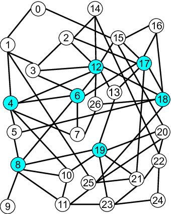


In this section, we formally define the Hub-Network (Subsection 4.1) and present an efficient approach to discover it (Subsection 4.2).
To facilitate our discussion, we first introduce the following notation. Let be a graph where is the vertex set and is the edge set. The edge from vertex and is denoted by , and we use to denote a simple path between and . The length of a simple path is the number of edges in the path, denoted by . Given two vertices and , their shortest path is the path between them with the minimal length. The distance from vertex to is the length of shortest path between and , denoted by . Note that for a directed graph, the edge set may contain either , , or both. For an undirected graph, the edge has no direction; in other words, it can be considered bidirectional, so the edge set contains either both edges and or neither of them. In undirected graph, the shortest path distance from to is equivalent to the one from to , i.e., . The techniques discussed in the paper can be applied both undirected and directed graph; for simplicity, we will focus on the undirected graph and we will briefly mention how each technique can be naturally extended to handle directed graphs.
4.1 Distance-Preserving Subgraph and Hub-Network
Intuitively, a hub-network is a minimal subgraph of the original , such that at least one shortest path between two hubs can be recovered in the subgraph (the distance is preserved). To formally define the hub-network, we first introduce the concept of distance-preserving subgraph and its discovery.
Definition 1
Distance-Preserving Subgraph Given graph and a set of vertex pairs , a distance-preserving subgraph of ( and ) has the following property: for any , , where and are the distances in subgraph and original graph , respectively.
Given a collection of vertex pairs whose distance need to be preserved in the subgraph, the subgraph discovery problem aims to identify a minimal subgraph in terms of the number of vertices (or edges).
Definition 2
Minimal Distance-Preserving Subgraph
(MDPS) Problem
Given graph and a set of vertex pairs , the minimal distance-preserving subgraph (MDPS) problem aims to discover a minimal subgraph with the smallest number of vertices, i.e., , where is a distance-preserving subgraph with respect to .
Once all the vertices are discovered, the induced subgraph of is a candidate minimal subgraph. Note that its edge set may be further sparsified. However, the edge sparsification problem with respect to a collection of vertex pairs (equivalent to the minimal distance-preserving subgraph problem in terms of the number of edges) is equally difficult as the MDPS problem (see discussion below); and the number of edges which can be removed are typically small in the unweighted graph. Thus, we will not explore the further edge reduction in this work.
Given graph and a set of hubs , let contain all the hub pairs whose distance is no greater than , then the hub-network is defined as the minimal distance-preserving subgraph of in .
Example 4.1
Note that an alternative approach is to build the weighted hub-network which explicitly connects the hub pairs: for instance, if any other hub lies in a shortest paths between two hubs, an edge can be added to directly link them. Indeed, most of the existing studies have adopted a similar approach to build and utilize some highway structure (but they target mainly road networks, which are rather sparse). However, this approach can lead to a number of problems when searching a massive social network: 1) Such hub-network would be weighted and could be dense (many new edges may need to be added between hubs) and to search through it, Dijkstra’s algorithm (or its variant) must be utilized and would be slower than BFS (because of using the priority queue). Higher edge density exacerbates this slowdown. 2) Bidirectional BFS is typically used to search an unweighted network and could be adopted to search the remaining network (excluding the hub-network). However, combining bidirectional BFS with Dijkstra’s can be rather difficult; 3) Significant memory may be needed to record such a hub-network as it is rather dense. Moreover, to recover the shortest path, additional information has to be recorded for each added new edge. Considering these issues, we utilize the distance-preserving subgraph as the hub-network, which does not induce additional memory cost, and can naturally support (bidirectional) BFS. Note that in Sections 5 and 6, we will study how to use more memory for higher query performance (without involving the difficulty of weighted hub-network).
To discover the hub-network in a massive social network, we need a fast solution for the Minimal Distance-Preserving Subgraph (MDPS) problem. However, finding the exact optimal solution is hard.
Theorem 1
Finding the minimal distance-preserving subgraph of a collection of vertex pairs in a graph is an NP-hard problem.
Proof Sketch: We reduce the set-cover decision problem r to the decision version of the minimal distance-preserving subgraph problem. In the set-cover decision problem, let be the ground set and records all the candidate sets, where for any candidate set and . The set-cover decision problem asks whether there are or fewer candidate sets in , such that .
Now we construct the following MDPS instance based on a set cover instance: consider a tripartite graph where the vertices in and have one-to-one correspondence to the elements in the ground set , and the vertices in one-to-one correspond to the candidate sets in . For simplicity, let (vertex () corresponds to element ); and let (vertex corresponds to candidate set ). Then, the edge set () contains all the edges () if element belongs to the candidate set . Note that the tripartite graph can be considered symmetric ( and ).
We claim that the set-cover decision problem is satisfiable if and only if the following MDPS problem is true: there is a subgraph with vertices to cover the shortest path distance of vertex pairs (), .
The proof of this claim is as follows. Assume the set-cover problem is satisfiable, let be the candidate sets which covers the ground set, i.e., . Let include all the vertices in corresponding to . It is easy to observe the induced subgraph of can recover the distances of all pairs (), . Note that their distances in the original graph and the induced subgraph are all equal to .
From the other direction, let be the subgraph with vertices which recovers the distances of these pairs. Since the vertices in the pairs have to be included in the subgraph (otherwise, the distance can not be explicitly recovered), the additional vertices can only come from the vertex set (there are in the vertex pairs from and ). Note that the distance of () in the original graph is and to recover that, a vertex in has to appear in the subgraph so that both and are in the subgraph (and in the original graph). This indicates the corresponding candidate set covers element . Since there are at most vertices in , there are at most candidates needed to cover all the ground set .
Based on similar reduction, we can also prove that finding the minimal distance-preserving subgraph in terms the number of the edges is also an NP-hard problem. Due to simplicity, we will not further explore this alternative in the paper.
4.2 Algorithm for Hub-Network Discovery
In the subsection, we will discuss an efficient approach for discovering the distance-preserving subgraph and the hub-network. To simplify our discussion, we focus on extracting the hub-network, though the approach is directly applicable to any collection of vertex pairs (and thus the general distance-preserving subgraph). Recall that in the hub-network discovery problem, given a set of hubs and a collection of hub-pairs whose distance is no more than (for -degree shortest path search), then the goal is to recover the distance for the pairs in using a minimal (distance-preserving) subgraph.
To tackle the hub-network (and the distance-preserving subgraph) efficiently, we make the following simple observation. For any vertex pairs in , if there is another hub , such that , then we refer to the vertex pair as a composite pair; otherwise, it is a basic pair, i.e., any shortest path connecting and does not contain a hub in . Let be the set of basic pairs. Given this, it is easy to see that if a subgraph can recover all the vertex pairs in , then it is a distance-preserving subgraph of (and thus the hub-network). This indicates that we only need to focus on the basic pairs () as the distances of composite pairs can be directly recovered using the paths between basic pairs.
Considering this, at the high level, the algorithm of the hub-network discovery performs a BFS-type traversal from each hub and it accomplishes the two tasks: 1) during the BFS, all basic pairs including , i.e., , , should be recognized and collected; and 2) once a basic pair is identified, the algorithm will select a “good” shortest path which consists of the minimal number of “new” vertices (not included in the hub-network yet). In other words, as we traverse the graph from each hub, we gradually augment the hub-network with new vertices to recover the distance (shortest path) of the newly found basic pairs.
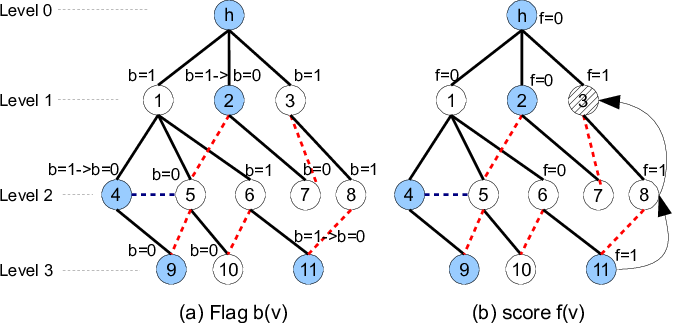
Recognizing basic pairs: To quickly determine whether the is a basic pair during the BFS process starting from hub , we utilize the following observation: Let vertex lie on a shortest path from hub to non-hub vertex with distance (i.e., is one hop closer than with respect to ). If there is a hub appearing in a shortest path from to ( and may not be distinct), definitely lies on a shortest path from to and is a composite pair (not basic pair). Based on this observation, we simply maintain a binary flag to denote whether there is another hub appearing in a shortest path between and . Specifically, its update rule is as follows: (not basic pair) if itself is a hub or ( is ’s parent in the BFS, i.e., and ). Thus, during the BFS traversal, when we visit vertex , if its flag (true) meaning there is no other hubs lying on the shortest path between and and we are able to recognize it is a basic pair.
Selecting a “good” shortest path between basic pairs: To select a good shortest path between basic pairs and , a basic measurement is the number of “new vertices” that need to be added to the hub-network. As a greedy criterion, the fewer that need to be added, the better is the path. To compute this, for any shortest path from starting point to , a score records the maximal number of vertices which are already in the hub-network. This measure can be easily maintained incrementally. Simply speaking, its update rule is as follows: if itself is in the hub-network or , where is ’s parent in the BFS (a shortest path from to go through and directly links to ). Also vertex records which has the maximal for tracking such a shortest path (with maximal number of vertices in the hub-network). Finally, we note that only for vertices with , i.e., when the shortest path between and does not go through any other hub, does a score need to be maintained. Otherwise, and its descendents cannot produce any basic pairs.
Overall Algorithm: The outline of this BFS-based procedure for discovering the hub-network is described in Algorithm 1. Here is the set recording the vertices in the hub-network. Initially, and then new vertices will be added during the processing. Note that in the queue for BFS traversal (Line ), we always visit those vertices with , i.e., they and any of their descendents (in the BFS traversal) will not form a basic pair, and thus the score does not need to be maintained for them. Once a hub is visited and it initially has , then is a basic pair (Line ); we will extract the shortest path which has the maximal number of vertices in the hub-network and add the new vertices to (Line ). Now, since the descendent of this hub (in the BFS traversal) will not form a basic pair, we simply change its flag to false, i.e., (Line ). Also, since we are only interested in the shortest path within -hop, we will not expand any vertex with distance to to be (Lines ). Before we expand the neighbors of , we also need to update its score based on whether itself is in the hub-network (Line ).
The complete expansion of a vertex is from Line to . We will visit each of its neighbors . If has not been visited, we will add it to the queue for future visiting (Line ). Then we perform the incremental update of flag and score . Flag will be turned off if (Line ) and if is larger than , i.e., the shortest path from to has the largest number of vertices so far in the hub-network. Vertex will record as the parent (for shortest path tracking) and is updated (Line ). This procedure will be invoked for each hub in .
 |
Example 4.2
Figure 2 illustrates the flag and score in the BFS process. Here the vertices , , , , and are hubs. In Figure 2 (a), , , and are basic pairs; the flag changes from originally to (Lines -). After the flag of ,, and changes to false (, all their descendents in the BFS traversal become false. For instance, the flag of vertex is false as it is also considered hub ’s descendent. In Figure 2(b), the shaded vertex indicates it is already included in the hub-network (). Therefore, vertex points to vertex (parent(11)=8 and parent(8)=3) as its score is higher than the that of vertex .
Theorem 2
If we invoke Algorithm 1 for each , then the induced subgraph is a hub-network of with respect to the -degree shortest path.
Proof Sketch: The correctness of the algorithm can be derived from the following two observations: 1) for any basic pair with distance no more than , there is at least one shortest path in as the algorithm explicitly extracts a shortest path and adds all its vertices to ; 2) for any composite pair with distance no more than , then it can always be represented as a sequence of basic pairs, which has at least one shortest path in . Thus, for any hub pair with distance no more than , their distance (at least one shortest path) is preserved in the induced subgraph .
The computational complexity for hub-network discovery as described in Algorithm 1 is basically equivalent to that of a simple BFS procedure. The overall procedure takes time, where is the hub set, and and are the number of vertices and edges, respectively, in ’s k-degree neighborhood. We also note that this algorithm works correctly for both undirected and directed graphs. Interestingly, we note the following property of applying Algorithm 1 for an undirected graph.
Lemma 1
Let be a basic hub pair in an undirected graph. Consider Algorithm 1 performs BFS from first and it discovers the shortest path . When it performs BFS from and discovers the symmetric basic pair , the algorithm will not add any additional new vertices.
Proof Sketch: The score guarantees = and thus a shortest path as “good” as will be extracted which does not need to add any new vertices to .
This observation leads to the simple bound constraint of the hub-network (the final size of ) and the result of Algorithm 1 will match such a bound.
Lemma 2
Let be the set of all unique basic hub pairs whose distance is no more than , then,
where is the average numnber of basic pairs per hub.
Proof Sketch: The term corresponds to the definition that any basic pair needs to recover only one shortest path; this also corresponds to the worst case scenario in Algorithm 1, where for any basic pair, all non-hub vertices along a new shortest path need to be added to . Note that for undirected graph treats basic pairs and as a single one. This directly leads to the term , which contemplates the maximal distance between any basic hub pair is and only one shortest path needs to be recovered for symmetric basic pairs and . Algorithm 1 also holds that (Lemma 1). Note that the result holds for directed graph as well where is the total degree of both incoming and outgoing edges.
5 Hub-Network based Search
In this section, we describe the hub-network based bidirectional BFS. The main challenge here is given a hub-network, how we can leverage it to maximally reduce the expansion of hubs and still guarantee to discover the correct -degree shortest path? Recall that a key reason for introducing the hub-network is to use it to constraint the expansion of hubs. Thus, a basic search principle is that any hub will only visit its neighbors in the hub-network. But what about any non-hub vertices in the hub-network, such as ? Should they be expanded only within the hub-network or should they be treated as the remaining vertices outside the hub-network? Furthermore, in traditional bidirectional BFS, when two searches (forward and backward) meet for the first time, the shortest path is discovered. Unfortunately, this does not necessarily hold if the hub is not fully expanded and thus the question becomes: what should be the correct stop condition? The stop condition is crucial as it determines the search space and the correctness of discovering the exact shortest path.
In the following, we first describe the hub-network based bidirectional BFS algorithm (Subsection 5.1) and then we prove its correctness and discuss its search cost (Subsection 5.2).
5.1 HN-BBFS Algorithm
The Hub-Network based Bidirectional BFS (HN-BBFS) algorithm consists of a two-step process: 1) (Meeting step) A bidirectional search will traverse both hub-network and remaining graphs until the forward and backward searches meet at the first common vertex; 2) (Verification step) Next, the searches continues in the remaining graphs (not hub-network) to verify whether the path discovered in the first step is shortest. If not, this step will discover an alternative shortest path.
Expansion Rule: In the Meeting step, the forward (backward) BFS follows the following rules to expand vertex in : 1) if a vertex is a hub, then it only expands its neighbors in the hub-network; 2) if a vertex is a regular vertex (not in the hub-network), then it expands all its neighbors; 3) for a vertex is a non-hub vertex but in the hub-network, , if the BFS traversal first reaches it through a hub, then it only expands its neighbors in the hub-network; otherwise, it is considered a regular vertex (no shortest path from start (end) vertex to it going through a hub). In the Verification step, both forward and backward BFS traversals will continue but they will not need to expand any hub, and any regular vertex and non-hub vertices in the hub-network will expand all their neighbors in the entire network.
Stop Condition: The stop condition for the forward (backward) BFS in the Verification step is as follows. Let be the shortest path distance discovered so far; let () be the distance between () to its closest hub ; let () be the current level being traversed by forward (backward) BFS. Then, the forward (backward) BFS will stop when the following condition is met:
| (1) |
Overall Algorithm: Hub-Network based Bidirectional BFS (HN-BBFS) is sketched in Algorithm 2. Note that BackwardSearch is essentially the same as ForwardSearch and is omitted for simplicity. Initially, is set to be for -degree shortest path search (indicating no path within -hops) and the condition is false (Line ).
The first step (Meeting Step) is carried out by the first while loop (Lines ), where a forward search and a backward search are employed in an alternating manner. In ForwardSearch (and BackwardSearch), a vertex in the corresponding queue () is expanded. The expansion rule as described earlier is used in Line . Basically, if a vertex is a hub or is in the hub-network, , but the BFS traversal first reaches it through a hub (there is a shortest path from to via a hub), it is considered “in-hub-network”. Otherwise, it is “out-hub-network”. For an in-hub-network vertex, BFS only expands its neighbors in the hub-network. Note that recognizing these “in-hub-network” vertices is straightforward and can be incrementally computed (similar to using the flag in Algorithm 1). Once a forward (backward) search visits a vertex already visited by the backward (forward) search, a candidate shortest path is discovered and is set to be true. Note that when is false (at the first step), every vertex (both hubs and non-hubs) will be visited and expanded.
Once turns true, the second step (Verification Step) is carried out by the second while loop (Lines ). Before the forward stop condition is met ( is false), the ForwardSearch will continue. However, only out-hub-network vertices will be visited and expanded (Line and Lines ). Also, during the expansion process, the candidate shortest path can be updated (Lines ). Finally, when the stop condition is met (Line : is the current BFS level being expanded, thus ), will become true and no forward search will not performed (Line ). Note that () can be easily computed during the BFS traversal: the first time a hub is visited, its distance to is recorded as .
5.2 Correctness and Search Cost
We now discuss the correctness of HN-BBFS (Algorithm 2) and then its search cost (especially in terms of the new Stop condition, Formula 1). To prove the correctness of HN-BBFS, we will make the following important observations:
Lemma 3
For any hub , during the first step (Meeting Step), the distance computed using the forward BFS search, i.e., the number of traversal levels to reach , is the exact shortest path distance between and . The same holds for for the backward BFS traversal.
Proof Sketch: If is a hub, then based on the hub-network definition, this clearly holds. If is not a hub, then one of the following two cases must hold: 1) All shortest paths between do not contain a hub except , so the forward BFS finds the shortest path distance by traversing only non-hub vertices in the original graph; 2) There is a shortest path between containing another hub, so there is always , such that does not contain any hubs and can be discovered in the hub-network.
Lemma 3 demonstrates the power of the hub-network and shows that HN-BBFS can correctly calculate the shortest path (distance) between query vertices to hubs (and between hubs). However, despite this, the candidate shortest path being discovered at the first meeting vertex may not be the exact one. The following lemma categorizes the exact shortest paths if they are shorter than the candidate shortest path discovered in the first step (Meeting Step).
Lemma 4
Assuming is the meeting vertex where forward and backward search first meet (Lines in Algorithm 2), the candidate shortest path is denoted as and the distance is . If there is a shorter path, then it must contain a hub , such that the exact shortest path can be represented as two segments and . Moreover, either 1) contains no hub other than with distances and , or 2) contains no hub other than with distances and .
Proof Sketch: We prove this by way to contradiction. It the lemma does not hold, then the following two types of paths cannot be shorter than the discovered candidate shortest path: 1) there is no hub in the exact shortest path , and 2) there are two hubs and , such that the shortest path has three segments: , and where and . For the first case, the bidirectional BFS should be able to find such a path (if they are shorter than the candidate ) earlier as it only involves visiting non-hub vertices in the graph. For the second case, based on Lemma 3, Algorithm 2 computes the exact and before the two BFS met at and the hub-network encodes the correct distance between . Thus, if , this shortest path should be discovered (met at an in-hub-network vertex) during the first step (Meeting Step). Since both cases are impossible, the lemma holds.
Theorem 3
The Hub-Network based Bidirectional BFS approach (HN-BBFS, Algorithm 2) guarantees the discovery of the exact -degree shortest path.
Proof Sketch: Basically, we need show that when the stop condition is met, no shorter alternative paths exists. By Lemma 4, if a shortest path exists that is better than the candidate shortest path ), it must follow one of two simple formats. These formats suggest we only need to extend out-hub-network vertices until they meet a hub already visited from the other direction ( or ). If such a path can be found, it must be shorter than the already discovered distance , i.e., (the best case situation is when the shortest path extends from the current step by one step to a hub closest to the query vertices). Clearly, if this does not hold, any shortest path in this format will not be smaller than .
In classical Bidirectional search, once both directions meet at a common vertex, the search can be stopped and the exact shortest path is discovered. However, in HN-BBFS, in order to reduce the expansion of hubs, some additional traversal (Verification Step) has to be taken. Clearly, if we need to walk additional steps, then the benefit of HN-BBFS can be greatly compromised.
So, what is the average number of steps HN-BBFS needs to take for a typical (random) query in the Verification step? The number is close to or at most one. To illustrate, first consider the distance between two vertex pairs to be (since most distances are less than that in social networks [39]), and assume and are not hubs (because there are few hubs) but each of them has a direct hub-neighbor (). Note that both directions typically traverse at most three steps, i.e., . Thus, at most one extra step needs to be taken in this case to make the stop condition true: , where . Similarly, let us consider the distance to be and assume each direction has taken steps in the Meeting Step. In this case, there is no need to take an additional step (assuming and are not hubs), and we can immediately recognize that the candidate shortest path is indeed the exact one. Finally, we note that when , i.e., the last step of BFS for Verification, there is no need to expand all the neighbors of a given vertex. Only its immediate hub-neighbors need to be expanded and checked (Lemma 4 and Theorem 3). To facilitate this, the neighbors of regular vertices can be reorganized so that the hub-neighbors and non-hub-neighbors are separately recorded.
6 Hub2-Labeling for Shortest Path Computation
In this section, we present a Hub2-labeling approach which aims to completely avoid visiting (and expanding) any hub. To achieve this, more expensive though often affordable pre-computation and memory cost are utilized for faster online querying processing. In Subsection 6.1, we will describe the Hub2-labeling framework and its index construction. In Subsection 6.2, we will discuss the faster bidirectional BFS.
6.1 Hub2-Labeling Framework
Hub2-Labeling replaces the Hub-Network with a Hub2 distance matrix and Hub Labeling.
Hub2: The distance matrix between hub pairs (referred to as Hub2) is precomputed and stored in main memory. Indeed, only the distances of pairs with distance no more than need to be computed for -degree shortest path. As we discussed before, nowadays a desktop computer with moderate memory size can easily hold such a matrix for (or more) of hubs.
Hub Labeling: In order to effectively utilize the distance matrix, each vertex in the graph also records a small portion of hubs, referred to as the core-hubs, along with the distances. Basically, those core-hubs along with the distance matrix can help quickly estimate the upper-bound of distance between the query vertex pairs and can be used for bounding the search step of bidirectional BFS.
Now, we formally define the core-hubs.
Definition 3
(Core-Hubs) Given graph and a collection of hubs, for each vertex , we say vertex is a core-hub for if there is no other hub such that . Formally, .
Simply speaking, if no other vertex appears in any shortest path between and , is ’s core-hub. Note that a pair , where , is similar to a basic pair in the hub-network (Subsection 4.2). The original basic pair definition only refers to hub pairs, but here it is being extended to vertex pairs with one hub and one non-hub vertex.
Example 6.1
Using the core-hubs and distance-matrix Hub2 , we can approximate the distance and the shortest path for vertex pair in the following fashion:
| (2) |
Here, is the exact distance recorded in the distance-matrix Hub2.
The construction of the distance matrix Hub2 and the labeling of core-hubs are also rather straightforward. The BFS procedure in Algorithm 1 can be easily adopted: 1) each BFS performs steps and thus the distance matrix can be directly constructed; 2) when a vertex has flag (basic pair) from BFS traversal of , we simply append to . Thus, the total computational complexity of the pre-computation is time, where is the hub set and and are the number of vertices and edges, respectively, in ’s k-degree neighborhood. We note that for directed graphs, we will compute both and , one for incoming core-hubs and the other for outgoing core-hubs . To construct such labels, we need perform both forward and backward BFS from each hub.
The overall memory cost of Hub2-Labeling is the sum of the cost of the distance matrix (Hub2) together with the core-hub labeling for each vertex (): . This turns out to be rather affordable. In the experimental study, we found that for most of the real social networks, the core-hubs of each vertex is only a small portion of the total hubs (in most case, less than or close to ). Thus, the Hub2-Labeling can easily handle graphs with more than hubs. Furthermore, since the second term (the size of the distance matrix) is stable, as the number of vertices increases in the original graph, the first term will scale linearly with respect to .
6.2 Hub2-Labeling Query Processing
To compute the -degree shortest path between vertex pair , the online query process in Hub2-Labeling consists of two steps:
Step 1 (Distance Estimation): Using the distance matrix Hub2 and core-hubs labeling and , the distance is estimated (Formula 2).
Step 2 (Hub-Pruning Bidirectional BFS (HP-BBFS)): A bidirectional BFS from and is performed and the search step is constrained by the minimum between (for -degree shortest path) and . In particular, none of the hubs need to be expanded during the bidirectional search. Mathematically, the Hub-Pruning Bidirectional BFS is equivalent to performing a typical Bidirectional BFS on the non-hub induced subgraph, of .
Theorem 4
The two-step Hub2-Labeling query process can correctly compute the -degree shortest path in graph .
Proof Sketch: We observe that any vertex pair with distance no more than can be categorized as: 1) vertex pairs having at least one shortest path passing through at least one hub in ; and 2) vertex pairs whose shortest paths never pass through any hub.
For any vertex pair with distance no greater than (), if there exists one hub satisfying , then, we can always find and such that . In other words, Step (distance estimation), which uses the distance-matrix Hub2 and core-hub labeling, can handle this category. Also, the Step will help confirm the shortest path belongs to this category (cannot find a shorter one).
If an approximate shortest path computed in Step is not an exact one, then the shortest path does not involve any hub. Thus Step can guarantee to extract an exact shortest path using the bidirectional search in the non-hub induced subgraph .
The time complexity of online query processing of a pair and can be written as + + ++ ), where is the distance estimation cost and the remaining terms are the cost of bidirectional search. () and () are the number of vertices and edges in the -neighborhood (reversed neighborhood which follows the incoming edges) of the non-hub induced subgraph . Since the hubs are excluded, the cost of hub-pruning bidirectional BFS is significantly smaller than that on the original graph.
However, if the number of core-labels is large, then the distance estimation can be expensive (a pairwise join on and is performed). To address this issue, the core-hubs in can be organized in a level-wise fashion, each level corresponding to their distance to , such as . Using such a level-wise organization, we can perform a much more efficient distance estimation: the pairwise joins first performed between and ; then on , , , etc. Given this, let us denote to be the shortest path length obtained by pairwise join so far. Assuming we are currently working on , if , then we terminate the pairwise join immediately. This is because it is impossible for to produce better results since . This early termination strategy based on the level-wise organization can help us effectively prune unnecessary pairwise join operations and improve the query efficiency.
7 Experimental Evaluation
In this section, we empirically evaluate the performance of our algorithm on a range of large real social networks. In particular, we will compare the Hub-Network approach (denoted as HN) and Hub2-Labeling approach (denoted as HL) with the following methods: 1) basic breadth-first search (denoted as BFS); 2) bidirectional breadth-first search (denoted as BiBFS); 3) the Sketch algorithm [9] (denoted as S⋆), the state-of-the-art approximate distance estimation algorithm; 4) the TreeSketch method [16] (denoted as TS⋆), which utilizes a tree to improve the approximation accuracy of Sketch based shortest path computation. Here the symbol also indicates it is an approximation method.
In addition, we have also tested the two latest exact shortest path distance methods, including tree decomposition based shortest path computation [40] and the highway-centric labeling approach [19] based on authors’ provided implementation. However, neither of them can work on the graphs used in this study. This is as expected as their indexing cost is very high (tree decomposition or set-cover approach) and they are mainly focusing on very sparse graphs.
We also tested RigelPath, another recent approach on approximate shortest path discovery in social networks [42]. However, its query performance is slower than that of Sketch (also confirmed in their own study [42]). Furthermore, its current implementation only focuses on undirected graphs, wheres most of the real benchmarking networks are directed. Thus, we do not report RigelPath’s experimental results here.
We implemented our algorithms in C++ and the Standard Template Library (STL). The implementation of sketch-based approaches (including S∗ and TS∗) is kindly provided by authors [16] (also implemented in C++). All experiments were run on a Linux server with 2.48GHz AMD Opteron processors and 32GB RAM.
In experiments, we are interested in two important measures: query time and preprocessing cost, which consists of precomputation time and indexing size. To measure the query time, we randomly generate vertex pairs and obtain the average running time for each query. For the index size, since all Sketch indices are stored in RDF format, their indexing sizes are measured in terms of the corresponding RDF file size. If the preprocessing cannot be finished in hours,we will stop it and record “-” in the table of results. Furthermore, we note that all Sketch-based benchmarks can only approximate shortest paths, where approximation accuracy is influenced by an iterative sampling procedure. A parameter is specified to determine the number of sampling iterations, which leads to sketches for each vertex. To make a fair comparison with exact query schemes, we set as suggested in [16] which can produce sketches with good approximation accuracy and efficient query processing. Also, in this study, we focus on comparing their query time again the new approaches despite they are only able to provide approximate solution whereas our approaches can provide the exact solution.
| Dataset | ||||
|---|---|---|---|---|
| 63731 | 1545686 | 48.51 | 8.2 | |
| Slashdot | 82168 | 948464 | 23.09 | 4.7 |
| BerkStan | 685230 | 7600595 | 22.18 | 10 |
| Youtube | 1138499 | 4945382 | 8.69 | 7.14 |
| As-skitter | 1696415 | 11095298 | 13.08 | 5.9 |
| Flickr | 1715255 | 22613981 | 26.37 | 7.32 |
| Flickr-growth | 2302925 | 33140018 | 28.78 | 7.19 |
| Wiki-talk | 2394385 | 5021410 | 4.19 | 4 |
| Orkut | 3072441 | 223534301 | 145.51 | 5.7 |
| LiveJournal | 5204176 | 77402652 | 29.75 | 8.34 |
| 11316811 | 85331845 | 15.08 | 24.97 |
| Dataset | ||||||||
|---|---|---|---|---|---|---|---|---|
| HN | HL | HN | HL | HN | HL | HN | HL | |
| 0.043 | 0.018 | 0.044 | 0.017 | 0.042 | 0.017 | 0.040 | 0.019 | |
| Slashdot | 0.023 | 0.002 | 0.021 | 0.001 | 0.022 | 0.001 | 0.022 | 0.002 |
| BerkSta | 0.011 | 0.005 | 0.005 | 0.009 | 0.010 | 0.004 | 0.014 | 0.002 |
| Youtube | 0.106 | 0.006 | 0.119 | 0.005 | 0.125 | 0.005 | 0.136 | 0.005 |
| As-skitter | 0.051 | 0.016 | 0.044 | 0.015 | 0.040 | 0.013 | 0.041 | 0.011 |
| Flickr | 1.600 | 0.112 | 1.671 | 0.073 | 1.739 | 0.067 | 1.888 | 0.061 |
| Flickr-growth | 0.998 | 0.138 | 1.130 | 0.113 | 1.193 | 0.100 | 1.236 | 0.136 |
| Wiki-talk | 0.014 | 0.002 | 0.016 | 0.002 | 0.014 | 0.002 | 0.014 | 0.001 |
| Orkut | 0.952 | 3.653 | 0.955 | 3.314 | 0.978 | 3.356 | 1.078 | 3.282 |
| LiveJournal | 0.466 | - | 0.526 | - | 0.513 | - | 0.577 | - |
| 1.850 | 0.306 | 1.947 | 0.314 | 2.083 | 0.340 | 2.121 | - | |
| Dataset | BFS | S∗ | TS∗ | BiBFS | HN | HL |
|---|---|---|---|---|---|---|
| 1.7 | 0.5 | 20.4 | 55.2 | 41.9 | 17.4 | |
| Slashdot | 1.4 | 0.7 | 34.5 | 31.6 | 22.2 | 1.3 |
| BerkStan | 0.3 | 4.7 | 559.1 | 33.9 | 10.2 | 3.5 |
| Youtube | 15.3 | 2 | 171.2 | 312.2 | 125.1 | 5.4 |
| As-skitter | 4.9 | 1.5 | 114.9 | 86.7 | 40.4 | 12.7 |
| Flickr | 42.6 | 2.7 | 288.7 | 2887.9 | 1738.8 | 67.3 |
| Flickr-growth | 71.8 | 5.1 | 305 | 1607.4 | 1193.3 | 100.3 |
| Wiki-talk | 18.8 | - | - | 56.4 | 14.1 | 1.5 |
| Orkut | 202.5 | 7.8 | 258.5 | 1338.7 | 978.1 | 3356.4 |
| LiveJournal | 131.4 | - | - | 749.6 | 513.1 | - |
| 221.4 | - | - | 2311.8 | 2082.6 | 339.7 | |
| Dataset | BFS | S∗ | TS∗ | BiBFS | HN | HL |
|---|---|---|---|---|---|---|
| 1.9 | 0.5 | 19.6 | 61.2 | 45.7 | 19.9 | |
| Slashdot | 1.7 | 0.7 | 46.8 | 31.4 | 20.3 | 1.5 |
| BerkStan | 0.3 | 2.1 | 206.7 | 36.1 | 10.6 | 3.8 |
| Youtube | 16 | 1.2 | 95 | 325.8 | 130.7 | 5.6 |
| As-skitter | 5.4 | 1.2 | 84.2 | 94.7 | 46.3 | 14 |
| Flickr | 45.2 | 2.9 | 182.1 | 3060 | 1825.2 | 79.1 |
| Flickr-growth | 71.9 | 3.7 | 332.5 | 1616.6 | 1219.6 | 103.6 |
| Wiki-talk | 21.7 | - | - | 58.3 | 14.2 | 1.1 |
| Orkut | 225.8 | 3.4 | 268 | 1372.9 | 1111.1 | 4639.5 |
| LiveJournal | 127.7 | - | - | 699.3 | 524 | - |
| 250.4 | - | - | 2384.3 | 2190.1 | 254.5 | |
| Dataset | BFS | BiBFS | HN | HL | |
|---|---|---|---|---|---|
| HP-BBFS | Join | ||||
| 30589 | 1723 | 1867 | 208 | 466 | |
| Slashdot | 41030 | 1380 | 1358 | 3 | 20 |
| BerkStan | 11099 | 1462 | 405 | 78 | 39 |
| Youtube | 505842 | 13941 | 6303 | 78 | 90 |
| As-skitter | 161878 | 3580 | 1551 | 292 | 265 |
| Flickr | 580315 | 36161 | 15494 | 1431 | 1330 |
| Flickr-growth | 777994 | 23738 | 12412 | 2382 | 1431 |
| Wiki-Talk | 1178526 | 4255 | 1111 | 1 | 7 |
| Orkut | 1522640 | 29341 | 21954 | 71331 | 5367 |
| LiveJournal | 1784211 | 14172 | 15554 | - | - |
| 3275797 | 55558 | 54884 | 13866 | 10757 | |
| Dataset | Indexing Cost | Preproc.Time(min) | ||||
|---|---|---|---|---|---|---|
| S∗(MB) | HLall(MB) | S∗ | HN | HL | ||
| 10 | 955 | 8.2 | 3.2 | 2.2 | 3.8 | |
| Slashdot | 26 | 496 | 11.1 | 6.5 | 1.3 | 4.3 |
| BerkStan | 193 | 291 | 21.6 | 64.3 | 0.3 | 1.7 |
| Youtube | 217 | 757 | 38.9 | 100.8 | 15.5 | 66 |
| As-skitter | 391 | 1229 | 101.9 | 109.9 | 7.1 | 31.7 |
| Flickr | 626 | 1536 | 232 | 163.8 | 43.4 | 202.5 |
| Flickr-growth | 1004 | 4403.2 | 315.9 | 242.8 | 71.8 | 363.5 |
| WikiTalk | - | 481 | 2.5 | - | 12.5 | 41.2 |
| Orkut | 8397 | 13517 | 749.3 | 773.2 | 412.5 | 1431.6 |
| LiveJournal | - | - | - | - | 334.2 | - |
| - | 26931 | 464 | - | 233.9 | 390.2 | |
| Dataset | ||||||||||||
|---|---|---|---|---|---|---|---|---|---|---|---|---|
| 20854 | 247.7 | 217.1 | 27364 | 202.7 | 184.5 | 30554 | 182.2 | 168.1 | 36188 | 146.6 | 137.5 | |
| Slashdot | 23359 | 204.5 | 179.5 | 27581 | 150.1 | 135.6 | 29500 | 128.4 | 117.2 | 32665 | 95.2 | 88.0 |
| BerkStan | 8290 | 769.3 | 177.8 | 16563 | 574.3 | 152.8 | 24618 | 492.8 | 138.1 | 34342 | 364.6 | 110.3 |
| Youtube | 49516 | 587.5 | 299.9 | 69474 | 429.9 | 254.9 | 76894 | 369.4 | 231.1 | 100595 | 279.2 | 189.3 |
| As-skitter | 41371 | 958.9 | 211.0 | 56245 | 701.3 | 184.8 | 64785 | 601.4 | 171.3 | 82439 | 453.0 | 146.3 |
| Flickr | 19198 | 2539.3 | 1433.3 | 32972 | 2005.8 | 1364.7 | 42312 | 1776.7 | 1295.0 | 63774 | 1403.7 | 1128.9 |
| Flickr-growth | 22715 | 3175.3 | 1626.7 | 38819 | 2555.4 | 1615.5 | 49450 | 2284.0 | 1565.4 | 74569 | 1833.5 | 1407.7 |
| Wiki-talk | 24139 | 984.5 | 294.7 | 32435 | 669.2 | 220.3 | 36081 | 552.4 | 188.8 | 41567 | 385.9 | 139.9 |
| Orkut | 124607 | 3808.5 | 1720.9 | 189686 | 3022.9 | 1763.0 | 225678 | 2734.3 | 1763.4 | 319989 | 2305.0 | 1720.0 |
| LiveJournal | 151348 | 1172.3 | 702.1 | 229836 | 1004.5 | 673.4 | 278203 | 932.8 | 653.7 | 392423 | 808.8 | 611.0 |
| 201521 | 9556.6 | 2877.8 | 346091 | 6762.9 | 2641.2 | 424853 | 5749.2 | 2463.3 | 564435 | 4267.5 | 2084.0 | |
The benchmarking datasets are listed in Table 2. Most of them are gathered from online social networks, with the number of vertices ranging from several tens of thousands to more than million. Others also exhibit certain properties commonly observed in social networks, such as small diameter and relatively high average vertex degree. All datasets are downloadable from Stanford Large Network Dataset Collection 11 1 http://snap.stanford.edu/data/index.html, Max Planck Institute’s Online Social Network Research Center 22 2 http://socialnetworks.mpi-sws.org/, and Social Computing Data Repository at Arizona State University 33 3 http://socialcomputing.asu.edu/datasets/.
In Table 2, we present important characteristics of all real datasets, where is average vertex degree (i.e., ) and is 90-percentile effective diameter [24]. Finally, in the experimental study, we focus on the -degree shortest path queries () as they are the most commonly used and also the most challenging one.
7.1 Experimental Results
In the following, we report effectiveness and efficiency of the shortest path computation algorithms from different perspectives:
Query Results on Random Queries In this experiment, we randomly generate vertex pairs with various distances and execute all algorithms on these queries to study their performance. Here, we select vertices with highest vertex degree as hubs. Table 4 presents the average query time for queries on all the methods and Table 4 highlights the average query time for those vertex pairs whose distance is no less than (longer path) as these are the more challenging ones (the longer the path, the likely more hubs will be expanded). Note that for BFS and two sketch methods Sketch(S∗) and TreeSketch(TS∗), we use the millisecond () as the unit, as they typically have much longer query time, and for BiBFS and our new approaches, Hub-Network (HN) and Hub2-Labeling (HL) approaches, we use the microsecond () as the unit, as they are much faster. Their corresponding average search space per query is reported in Table 6, where column “HP-BBFS” records the average number of vertices visited by HP-BBFS (Hub-Pruning Bidirectional BFS) in Hub2-Labeling (HL) and column “Join” records the average times of pairwise join on the core-hubs labeling and in HL. We make the following observations on the query time and average search space:
1) The Hub2-Labeling (HL) is clearly the winner among all algorithms, which is on average more than times faster than BFS. In most of the social networks, like As-skitter and WikiTalk, the average query time of Hub2-Labeling (HL) is only tens of microseconds ( second), and except for one (Orkut), all of tham are less than ms. Overall, Hub2-Labeling (HL) is on average times faster than BiBFS. Specifically, we observe that compared to BiBFS, the Hub-Pruning Bidirectional Search (HP-BBFS) of achieves significant improvement in terms of search space, which is around times smaller than BiBFS (Table 6).
2) The Hub-Network (HN) is on average about times faster than BiBFS (with no additional storage cost but reorganizes the network structure). It is about two orders of magnitude faster than BFS but is about times slower than the Hub2-Labeling approach.
3) Sketch (S⋆) is on average about times faster than BFS but it fails to run on a few datasets. The TreeSketch (TS⋆) is on average times slower than Sketch. Both Hub-Network and Hub-Labeling approaches are are on average more than two orders of magnitude faster than Sketch, the fastest approximation method.
4) For long distance queries the exact shortest path approaches require longer query time (Table 4). However, the increase for the Hub-Network (HN) and Hub2-Labeling (HL) are smaller than BFS and BiBFS. Also, it is interesting to observe the approximate shortest path approaches do not show performance decrease though both of them are still very slow.
Preprocessing Cost: Table 6 shows preprocessing cost of the Sketch-based approach along with HL, consisting of indexing size and precomputation time. The first column S⋆ records the index size (MB) for the Sketch method. The second column HLtotal records total index size of Hub2-Labeling (HL), which is the sum of core-hubs labeling cost and distance matrix size. Column record the average number of core-hubs stored by each vertex. Remarkably, the core-hub labeling scheme in Hub2-Labeling (HL) is very effective, as there is a very small portion of core-hubs recorded by each vertex. In most of the network, the average number of core-hubs per vertex is no more than of the total hubs. In particular, for network WikiTalk, only core-hubs are stored in each vertex on average, which potentially leads to efficient query answering. However, for LiveJournal, the Hub2-Labeling is too expensive to be materialized in the main memory. In terms of precomputation time, Hub2-Labeling can be constructed faster than Sketch on out of networks. The construction time of HubNetwork (HN) is average more than three times faster than the Hub2-Labeling (HL), and it does not need any additional memory cost.
Impacts of Hub Number: In this experiment, we study the effect of different number of hubs on query performance. Here, we vary the hub-set size from to and conduct the experiment on randomly generated queries with various distances. Table 2 shows the average query time of Hub-Network (HN) and Hub2-Labeling approaches using different number of hubs. In most of these networks, the best query performance is achieved when the number of hubs lies between and . Though a large number of hubs may potentially help reduce the search space of the bidirectional search in Hub2-Labeling (HL), it may also increase the size of core-hubs associated with each vertex. We observe that the query performance obtained by using hub is comparable to the best one). Note that here due to space limitation, we do not report the detailed precomputation cost in terms of construction time and index size (for Hub2-Labeling). Overall, as the number of hub increases, most large networks, show an increasing trend regarding the average index size. Interestingly, when hub-set size increases, significant reduction of average index size is observed on WikiTalk. This is in part explained by its very small diameter. In terms of the precomputation time, as more hubs are chosen, the computational cost of Hub-Network and Hub2-Labeling becomes larger, because more BFS needs to performed. Indeed, the precomputation time increases almost linearly with respect to the hub-set size.
Hub-Network Statistics: Finally, we report the basic statistics of the discovered distance preserving Hub-Network. Specifically, we are introduced in two following two questions: 1) given a set of hubs, how large the hub-network will be? What is the size of ? 2) what are the degree difference between the hubs in the original network and in the Hub-Network? Do we observe a significant degree decreasing? To answer these two questions, in Table 7, we report (the number of total vertices in the hub-network), the average degree of hubs in the original graph, and , the average degree of hubs in the extracted hub-network, with respect to , , and hubs. We observe for most graphs, the size of is a few times larger than the hub number; however, for Orkut, LiveJournal, and Twitter, the hub network becomes quite large at and hubs. Also, in general, the degree of hubs in the hub-network has been lowered and on several graphs, the average degree is reduced smaller than 1/3 of the original average degree. We also observe that the ability of lowering degree is correlated with the search performance: the better the hub degree is lowered, the better query performance improvement we can get from the Hub-Network based bidirectional BFS.
8 Conclusion
In this paper, we introduce a set of novel techniques centered on hubs for -degree shortest path computation in large social networks. The Hub-Network and Hub2-Labeling algorithms can help significantly reduce the search space. The extensive experimental study demonstrates that these approaches can handle very large networks with millions of vertices, and its query processing is much faster than online searching algorithms and Sketch-based approaches, the state-of-the-art shortest path approximation algorithms. To the best of our knowledge, this is the first practical study on computing exact shortest paths on large social networks. In the future, we will study how to parallelize the index construction and query answering process. We also plan to investigate how to compute -degree shortest path on dynamic networks.
References
- [1] I. Abraham, D. Delling, A. V. Goldberg, and R. F. Werneck. A hub-based labeling algorithm for shortest paths in road networks. In Proceedings of the 10th international conference on Experimental algorithms, 2011.
- [2] I. Abraham, A. Fiat, A. V. Goldberg, and R. F. Werneck. Highway dimension, shortest paths, and provably efficient algorithms. In SODA ’10, 2010.
- [3] H. Bast, S. Funke, P. Sanders, and D. Schultes. Fast Routing in Road Networks with Transit Nodes. Science, 316:566–, April 2007.
- [4] R. Bauer, D. Delling, P. Sanders, D. Schieferdecker, D. Schultes, and D. Wagner. Combining hierarchical and goal-directed speed-up techniques for dijkstra’s algorithm. J. Exp. Algorithmics, 15, March 2010.
- [5] James Cheng, Yiping Ke, Shumo Chu, and Carter Cheng. Efficient processing of distance queries in large graphs: a vertex cover approach. In SIGMOD Conference, pages 457–468, 2012.
- [6] James Cheng, Zechao Shang, Hong Cheng, Haixun Wang, and Jeffrey Xu Yu. K-reach: Who is in your small world. PVLDB, 5(11):1292–1303, 2012.
- [7] Edith Cohen, Eran Halperin, Haim Kaplan, and Uri Zwick. Reachability and distance queries via 2-hop labels. SIAM J. Comput., 32(5):1338–1355, 2003.
- [8] Reuven Cohen and Shlomo Havlin. Scale-free networks are ultrasmall. Phys. Rev. Lett., 90, Feb 2003.
- [9] A. Das Sarma, S. Gollapudi, and R. Najork, M.and Panigrahy. A sketch-based distance oracle for web-scale graphs. In WSDM ’10, 2010.
- [10] D.Djokovic. Distance-preserving subgraphs of hypercubes. Journal of Combinatorial Theory, Series B, 14(3):263 – 267, 1973.
- [11] D. Delling, P. Sanders, D. Schultes, and D. Wagner. Algorithmics of large and complex networks. chapter Engineering Route Planning Algorithms. 2009.
- [12] E. W. Dijkstra. A note on two problems in connexion with graphs. Numerische Mathematik, 1(1):269–271, December 1959.
- [13] Cyril Gavoille, David Peleg, Stéphane Pérennes, and Ran Raz. Distance labeling in graphs. J. Algorithms, 53(1):85–112, 2004.
- [14] R. Geisberger, P. Sanders, D. Schultes, and D. Delling. Contraction hierarchies: faster and simpler hierarchical routing in road networks. In Proceedings of the 7th international conference on Experimental algorithms, 2008.
- [15] A. V. Goldberg and C. Harrelson. Computing the shortest path: A search meets graph theory. In SODA ’05, 2005.
- [16] Andrey Gubichev, Srikanta Bedathur, Stephan Seufert, and Gerhard Weikum. Fast and accurate estimation of shortest paths in large graphs. In Proceedings of the 19th ACM international conference on Information and knowledge management, CIKM ’10, pages 499–508, 2010.
- [17] R. J. Gutman. Reach-based routing: A new approach to shortest path algorithms optimized for road networks. In ALENEX/ANALC, pages 100–111, 2004.
- [18] R. Jin, Y. Xiang, N. Ruan, and D. Fuhry. 3-hop: a high-compression indexing scheme for reachability query. In SIGMOD’09, 2009.
- [19] Ruoming Jin, Ning Ruan, Yang Xiang, and Victor E. Lee. A highway-centric labeling approach for answering distance queries on large sparse graphs. In SIGMOD Conference, pages 445–456, 2012.
- [20] N. Jing, Y. Huang, and E. A. Rundensteiner. Hierarchical encoded path views for path query processing: An optimal model and its performance evaluation. TKDE, 10(3):409–432, 1998.
- [21] S. Jung and S. Pramanik. An efficient path computation model for hierarchically structured topographical road maps. TKDE, 14(5):1029–1046, 2002.
- [22] J. Kleinberg, A. Slivkins, and T. Wexler. Triangulation and embedding using small sets of beacons. In FOCS ’04, 2004.
- [23] H. Kriegel, P. Kröger, M. Renz, and T. Schmidt. Hierarchical graph embedding for efficient query processing in very large traffic networks. In SSDBM ’08, 2008.
- [24] Jure Leskovec, Jon Kleinberg, and Christos Faloutsos. Graphs over time: densification laws, shrinking diameters and possible explanations. In ACM KDD ’05, pages 177–187, 2005.
- [25] Jure Leskovec, Kevin J. Lang, Anirban Dasgupta, and Michael W. Mahoney. Community structure in large networks: Natural cluster sizes and the absence of large well-defined clusters. CoRR, abs/0810.1355, 2008.
- [26] C. Castillo M. Potamias, F. Bonchi and A. Gionis. Fast shortest path distance estimation in large networks. In CIKM ’09, 2009.
- [27] Alan Mislove, Hema Swetha Koppula, Krishna P. Gummadi, Peter Druschel, and Bobby Bhattacharjee. Growth of the flickr social network. In Proceedings of the 1st ACM SIGCOMM Workshop on Social Networks (WOSN’08), August 2008.
- [28] T. S. Eugene Ng and H. Zhang. Predicting internet network distance with coordinates-based approaches. In INFOCOM, 2001.
- [29] Miao Qiao, Hong Cheng, Lijun Chang, and Jeffrey Xu Yu. Approximate shortest distance computing: A query-dependent local landmark scheme. In ICDE, 2012.
- [30] H. Samet, J. Sankaranarayanan, and H. Alborzi. Scalable network distance browsing in spatial databases. In SIGMOD’08, 2008.
- [31] P. Sanders and D. Schultes. Highway hierarchies hasten exact shortest path queries. In 17th Eur. Symp. Algorithms (ESA), 2005.
- [32] J. Sankaranarayanan, H. Samet, and H. Alborzi. Path oracles for spatial networks. PVLDB, 2, August 2009.
- [33] R. Schenkel, A. Theobald, and G. Weikum. HOPI: An efficient connection index for complex XML document collections. In EDBT, 2004.
- [34] S. Shekhar, A. Fetterer, and B. Goyal. Materialization trade-offs in hierarchical shortest path algorithms. In SSD ’97, 1997.
- [35] Y. Tao, C. Sheng, and J. Pei. On -skip shortest paths. In SIGMOD’11, 2011.
- [36] M. Thorup and U. Zwick. Approximate distance oracles. J. ACM, 52(1):1–24, 2005.
- [37] http://entitycube.research.microsoft.com.
- [38] http://www.6-degreeonline.com.
- [39] http://www.sysomos.com/insidetwitter/sixdegrees/.
- [40] Fang Wei. Tedi: efficient shortest path query answering on graphs. In SIGMOD Conference, pages 99–110, 2010.
- [41] Xiaohan Zhao, Alessandra Sala, Christo Wilson, Haitao Zheng, and Ben Y. Zhao. Orion: Shortest path estimation for large social graphs. In Proceedings of the 3rd Workshop on Online Social Networks (WOSN 2010), 2010.
- [42] Xiaohan Zhao, Alessandra Sala, Haitao Zheng, and Ben Y. Zhao. Efficient shortest paths on massive social graphs. In Proceedings of 7th International Conference on Collaborative Computing: Networking, Applications and Worksharing (CollaborateCom), 2011.