Mean-field embedding of the dual fermion approach for correlated electron systems
Abstract
To reduce the rapidly growing computational cost of the dual fermion lattice calculation with increasing system size, we introduce two embedding schemes. One is the real fermion embedding, and the other is the dual fermion embedding. Our numerical tests show that the real fermion and dual fermion embedding approaches converge to essentially the same result. The application on the Anderson disorder and Hubbard models shows that these embedding algorithms converge more quickly with system size as compared to the conventional dual fermion method, for the calculation of both single-particle and two-particle quantities.
pacs
02.70.-c, 71.27.+a, 71.10.Fd, 71.30.+hI Introduction
Mean-field methods like the Coherent Potential Approximation (CPA)[1, 2] and the Dynamical Mean-Field Theory (DMFT)[3, 4, 5, 6] are widely applied to the study of disordered and correlated materials. By construction, these methods are single-site mean-field approximations, where the real lattice is replaced by an impurity placed in a local (momentum-independent) effective medium. As single-site approximations, both the CPA and DMFT fail to take into account nonlocal inter-site correlations and fluctuations of the medium, which are found to be important in many materials with nonlocal order parameters or strong inter-site correlations.
To systematically incorporate such nonlocal corrections to these mean-field approaches, cluster extensions of the DMFT and CPA, such as the Dynamical Cluster Approximation (DCA)[7, 8, 9, 10] have been developed. Here a finite size periodic cluster of several lattice sites is placed in a self-consistently determined effective medium, which now acquires cluster-resolved momentum-dependence. The embedding is achieved by coarse graining the lattice problem in momentum space. Such a cluster embedding allows for explicit treatment of short-range correlations and non-local order parameters within the cluster size, while the longer length scale physics is still described at the mean-field level. The cluster may be solved with numerically exact methods such as quantum Monte Carlo or exact diagonalization. Unfortunately, these quantum cluster methods are limited by the computation effort needed for the cluster solvers. Exact diagonalization has an exponential scaling in cluster size and quantum Monte Carlo is plagued by the fermion sign problem [11].
To address such an exponential scaling, methods have been developed which map the lattice problem onto an impurity self-consistently embedded in a correlated lattice problem[12, 13, 14, 15]. Here, local correlations are treated on the impurity, while nonlocal correlations are incorporated on the lattice via a diagrammatic perturbation expansion around the DMFT solution. If a QMC method is used to solve the impurity problem, and if the impurity is small enough that the fermion sign problem is absent or controllable, then these methods scale algebraically in the lattice size. The dual fermion[15] approach is perhaps the most elegant of these methods since here the mapping to an embedded impurity is apparently exact, provided that the lattice perturbation theory can be solved to all orders.
One of the practical constraints in the implementation of the dual fermion method is that its computational complexity increases with the lattice size. The lattice size should be large enough to represent a thermodynamic limit, but this can make the diagrammatic calculation on the lattice computationally expensive. Becasue of such limitation the dual fermion approach has been applied mostly to one- and two-dimensional systems, and not yet to three-dimensional systems. To overcome this issue, we introduce an extension of the dual fermion method to include a third length scale introduced to reduce the complexity involved in the treatment of the correlations at the intermediate length scale. Here, using ideas from the DCA, the dual fermion lattice is replaced by a DCA cluster embedded in a self-consistently determined effective medium. Two algorithms are presented, one employs the DCA coarse graining on the real fermion lattice and the other on the dual fermion lattice. We find that the latter approach is more efficient and that this modification dramatically improves the convergence of the dual fermion method with system size and enables the use of higher order approximations for the diagrammatic solution to the cluster problem.
This paper is organized as follows. In Section II after reviewing the dual fermion algorithm, we provide a detailed description of the two proposed embedding schemes. Then in section III, to test our methods we first apply them to the one-dimensional Anderson disorder model. And in section IV, we demonstrate its application on the two-dimensional Hubbard model. The numerical results show a superior convergence of our embedding schemes as compared to the conventional dual fermion algorithm as a function of the lattice size. Section V summarizes and concludes the paper.
II Formalism
II.1 Dual fermion mapping
To derive the dual fermion formalism for either interacting [15] and disordered systems [16, 17], we start from the lattice action
| (1) |
where is the local part of the action (e.g., a Hubbard interaction term or a local disorder potential), and are Grassmann numbers corresponding to creation and annihilation operators on the lattice, is the chemical potential, is the lattice bare dispersion, and are the Matsubara frequencies. For interacting systems, this action is used to calculate the partition function [15] while for disordered systems the replica method may be used to directly calculate the Green functions [16, 17]. Then to express this action in terms of single impurity problem
| (2) |
we rewrite Eq. 1 as
| (3) |
here the impurity-excluded (bath) Green function is defined as and is the hybridization function between the impurity and the effective medium. By introducing the auxiliary (dual fermion) degrees of freedom via a Hubbard-Stratonovich transformation of the first term in Eq. 3, and then integrating out the real fermion degrees of freedom [15, 18] (see Appendix A in Ref. 18 for a detailed derivation), we end up with the following dual fermion action
| (4) |
where is the bare dual Green function defined as the difference between the DMFT and/or CPA lattice Green function and the impurity Green function , i.e.,
| (5) |
The dual fermion potential is parametrized by the many-body full vertex functions of the impurity problem defined by Eq. 2 (in practice, only the two-body vertex function is used) [15, 18]. In this way, the dual fermion lattice system is well-defined and thus provides sufficient input for a many-body diagrammatic calculation on the dual lattice. After the dual lattice action of Eq. 4 is solved, the dual fermion Green function is mapped back to the real fermion lattice via the relation of the form
| (6) |
This dual fermion formalism applies for both interacting and disordered [16, 17, 19] systems, provided that the dual potential is split into elastic and inelastic parts and the closed fermion loops involving the elastic parts only are eliminated to prevent unphysical renormalization of the interaction from scatterings from the disorder potential [16, 17].
II.2 Conventional Dual Fermion Algorithm
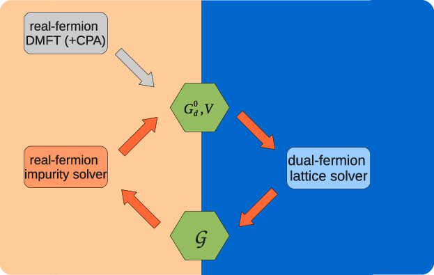
The conventional dual fermion algorithm is described in Fig. 1. We start from the DMFT and/or CPA solution of the real fermion system, and then use the information collected by solving the impurity problem (mainly the single-particle Green function , self-energy , and two-particle Green function ) to parametrize the dual fermion system, i.e. to construct the bare dual fermion Green function and the dual potential . While the local correlations are described by the DMFT and/or CPA solution, the nonlocal corrections are incorporated through the dual fermion part, which is calculated using standard perturbation expansion in the term. After the dual fermion system is solved, we map it back to real fermion system with the nonlocal corrections included in the lattice self-energy and Green function . We then solve the impurity problem again starting with an updated impurity-excluded Green function . These steps are repeated until self-consistency is achieved with , i.e. with the local contribution to the dual fermion Green function being zero [15].
There are two predominantly time-consuming parts in the dual fermion calculation. One is the calculation of the two-particle Green function in the impurity or cluster solver, where the time needed is fixed for a given parameter set. The other is the solution of the dual fermion lattice problem, where the time needed depends on the lattice size. Suppose the total system size is where is the number of frequencies used, is the linear lattice size and is the dimension. The total number of sites in the lattice is . Then the computational complexity of the dual fermion lattice calculation scales as
| (7) |
for a second-order calculation,
| (8) |
for a fluctuation exchange (FLEX) [20] calculation, and
| (9) |
for a two-particle self-consistent full parquet approach [21, 22]. To make sure that the calculation is representative of the thermodynamic limit, the lattice linear size should be around 100 sites or larger. This imposes a severe constraint on the application of the dual fermion approach which so far has been applied only on one- and two-dimensional systems, and not yet on three-dimensional systems. Even for one or two dimensions, the calculations are limited by the rapidly increasing computational complexity as the lattice size increases. Although the fast Fourier transform (FFT) might be used to reduce the computational complexity to and for the dual fermion second-order and FLEX calculations respectively, it is still very demanding when is large, and this reduction is not possible when using the parquet approach to solve the dual lattice problem.
Since the computational complexity depends on the linear size of the dual fermion lattice , we would like to reduce that value as much as possible. In the conventional dual fermion approach, both the real fermion and dual fermion lattices share the same linear size , so we would need to reduce the real fermion or the dual fermion system size. Note that after solving the impurity problem, the dual fermion lattice system is well-defined via the bare dual Green function and bare dual potential. In this sense, there is no difference as compared to the real fermion system. Thus, we can use any action-based approach available for the real fermion system to solve the dual fermion lattice problem. Using a second-order perturbation theory or FLEX for the conventional dual fermion approach can be interpreted as a finite-size calculation, and finite-size effects can be large. If we want to eliminate or reduce these finite-size effects, we can embed our dual fermion calculation in an effective medium. In the following, we will propose two such embedding schemes.
II.3 Real Fermion Embedding
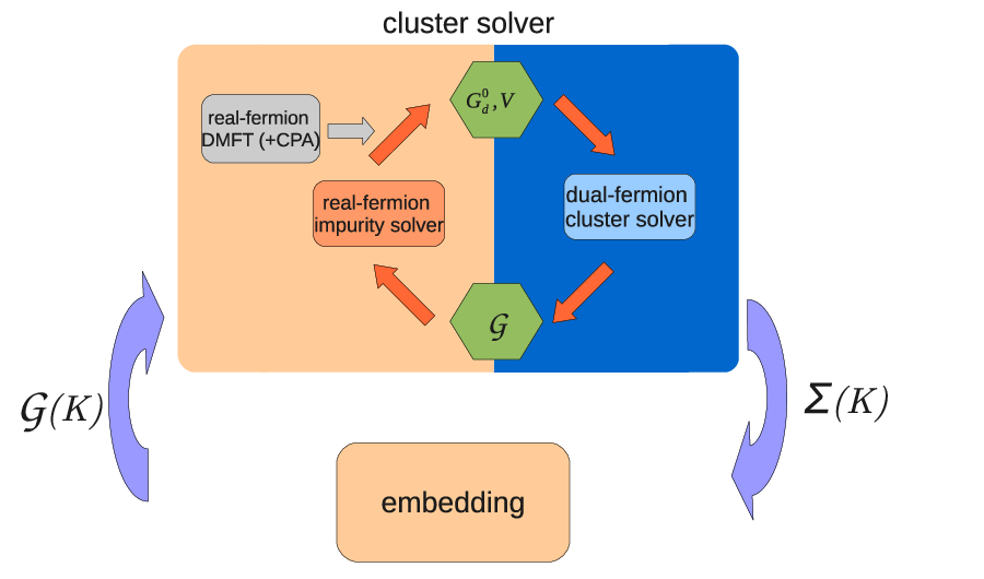
In the first approach, which we refer to as real fermion embedding, we use the concepts of coarse graining introduced in the DCA [7, 8] to map the real lattice to a cluster embedded in a self-consistently determined medium. However, unlike in the conventional DCA, here the cluster problem is solved using the dual fermion method (see Fig. 2). Therefore, we employ the conventional dual fermion approach as the DCA cluster solver where the cluster size can be chosen to be small, of the order of several dozen sites, and the cluster is embedded in a self-consistently determined real fermion mean field. If any momentum on the lattice and the cluster momentum are related as with labeling the momentum within a coarse-graining cell surrounding , then the coarse graining sums over are straightforward since the self-energy and irreducible vertices are assumed to be independent of . These sums may be completed in what is essentially the thermodynamic limit by a direct summation or, for single band models, by defining a partial bare single particle density of states. In either case the number of points can be chosen to be sufficiently large so that the thermodynamic limit is guaranteed in this algorithm. Note that in this embedding scheme the mean-field lives on a real fermion lattice. Therefore, after solving the cluster, any information collected from the dual fermion cluster should be mapped back to real fermion cluster. To be specific, the algorithm can be described as follows, where we suppress the explicit frequency dependence to simplify these expressions:
- •
Given the real fermion cluster self-energy which in the DCA scheme approximates the self-energy of the real lattice, we calculate the coarse-grained lattice Green function through:
(10) Then the cluster-excluded Green function is calculated by removing the cluster self-energy contribution
(11)
- •
With the calculated cluster-excluded Green function , the cluster problem is well-defined. The next step involves solving the cluster problem using a conventional dual fermion algorithm as the solver. Since here the ”lattice” for the conventional dual fermion approach is actually a cluster with linear size , which itself is embedded in a mean-field lattice, the original bare lattice Green function should be replaced accordingly by the cluster-excluded Green function:
(12) in Eq. 1. The parametrization of the dual fermion cluster problem is also affected with modified definition of the bare dual fermion Green function of Eq. as
(13) Notice that here, as in the conventional dual fermion scheme, the input to the dual fermion loop is constructed from the solutions of the impurity problem with impurity Green function and self-energy .
After the cluster problem is solved, we obtain the cluster real fermion Green function . The cluster self-energy then can be updated via the Dyson equation
(14)
We iterate these two steps until the difference between the self-energy from two consecutive iterations is below a given convergence criterion. Note that the real fermion cluster self-energy is used to approximate the lattice self-energy. For two-particle quantities, similarly, the real fermion irreducible vertex function is used to approximate the lattice irreducible vertex function and then the full vertex functions, two-particle Green functions and conductivity can be calculated accordingly [23].
II.4 Dual Fermion Embedding
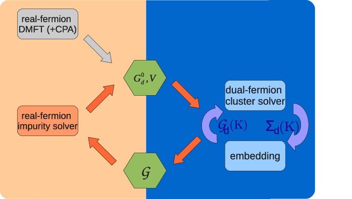
As an alternative to reduce the computational complexity in the dual fermion lattice calculation, we employ the DCA-like scheme on the dual fermion lattice directly. We refer to this approach as a dual-fermion embedding method, where the dual fermion lattice is replaced by a finite dual fermion cluster embedded in a self-consistently determined host. The proposed dual fermion embedding algorithm is described in Fig. 3.
The DCA algorithm for the dual fermion lattice is similar to the real fermion algorithm described above. Again taking the momentum on a cluster of size and the on the lattice, we can write down the dual fermion embedding algorithm as follows:
- •
Given the dual fermion cluster self-energy (either from an initial guess or from the previous iteration), we calculate the coarse-grained dual fermion lattice Green function through
(15) where the bare dual Green function is defined as
| (16) |
- •
We then calculate the cluster-excluded dual fermion Green function by removing the dual fermion cluster self-energy
| (17) |
- •
This dual fermion cluster-excluded Green function is the bare Green function on the dual fermion cluster, while the impurity full vertex is the bare dual interaction. Together, these two quantities define a perturbation theory that we may solve with various diagrammatic methods.
As an example, if the self-consistent second-order theory is used, we will iterate the following two equations:
(18) and
(19) until the self-consistency criterion for this inner loop is satisfied.
We can also use a simplified FLEX algorithm in which the self-energy is calculated from ladder summations where all scattering channels are treated on a equal footing. We calculate the two-particle quantities after the self-energy has converged by rotating these ladder contributions into the crossed channels using the parquet equations for the irreducible vertex functions. Details of the simplified FLEX method have been presented elsewhere [16, 12] and will not be discussed here.
After the DCA loop is converged and the dual lattice quantities are calculated, we continue as in the conventional dual fermion scheme, and use the obtained dual fermion quantities to parametrize their real lattice counterparts (e.g., Eq. 6), and repeat the whole procedure until self-consistency is reached.
III Results for Anderson disorder model
To qualify these new embedding schemes, we first apply them to the one-dimensional Anderson disorder model with the Hamiltonian
| (20) |
where only the nearest neighbor hopping, , is included, sets the unit of energy, and the on-site disorder potential is distributed according to
| (21) |
where is the step function
| (22) |
In the following, we will explore both single-particle and two-particle quantities using the dual fermion embedding algorithms described in Figs. 2 and 3.
III.1 Comparison of the two embedding schemes
T V RF embedding DF embedding conventional DF 0.05 1.0 4 2 2 0.05 2.0 4 2 2 0.01 1.0 6 2 2 0.01 2.0 5 2 2 0.005 1.0 9 2 2 0.005 2.0 7 3 3
Numerical tests show that, for most cluster sizes and within the convergence criterion, both the dual and real fermion embedding algorithms produce the same results for both single-particle and two-particle quantities. This is because the two approaches share many of the same features, including similar definitions of the impurity problem and the bare dual fermion interaction extracted from it. They differ mainly in the definition of the bare dual fermion Green function . As can be seen from Eqs. 10, 11 and 13 the bare dual Green function used in the real fermion embedding, , is dressed by the real fermion cluster self-energy , while from Eqs. 15 to 17 the bare dual Green function used in the dual fermion embedding algorithm is dressed by the dual fermion self-energy. Conceptually, these two self-energies differ in that the real fermion cluster self-energy includes both local and nonlocal single particle renormalization, while the dual fermion self-energy includes only nonlocal single particle renormalization. However, in both algorithms, the bare dual Green functions are formed from cluster-excluded Green functions, Eqs. 11 and 17 to prevent overcounting of the cluster diagrams, so that these Green functions are bare on the local cluster. So, at least conceptually, if not formally, the two bare Green functions contain the same information so that the two algorithms converge to nearly the same results.
However, the dual fermion embedding algorithm is a better choice. After the introduction of the embedding, the total time is generally dominated by the impurity solver, especially for the more realistic Hubbard-like model. The embedding in the real fermion scheme usually requires additional iterations of the impurity solver to achieve convergence. Table 1 shows a comparison of the number of times the impurity problem needs to be solved to obtain convergence by the two embedding algorithms and the conventional dual fermion algorithm. Indeed, generally the real fermion embedding algorithm needs 2 to 4 more iterations of the impurity solver than the dual fermion one. We also want to emphasize that the dual fermion embedding algorithm does not incur in additional iterations for the outer loop as compared to the conventional DF approach and thus does not increase the number of times the impurity problem is solved. Therefore, in the following, we only show results calculated using the dual fermion embedding algorithm.
III.2 System size dependence of the local Green function


Since the dual fermion formalism is a Green function based approach, we can analyze finite-size effects by looking into the local Green function at the lowest Matsubara frequency point ( is the system size)
| (23) |
Fig. 4(a) shows a comparison of results from both the conventional dual fermion and the dual fermion embedding algorithms at disorder strength and temperature . Results calculated from the conventional dual fermion approach oscillate and have a two-branch structure depending on whether , where the linear system size ( where is the dimension and here ), is an odd or even number. The linear system size has to be as large as 100 to achieve converged results. In contrast, the results from the embedding dual fermion algorithm converge very quickly with increasing cluster size and form a nearly flat line for the values of plotted. In addition, the oscillation and two-branch structure are absent, perhaps due to the fast convergence.
Fig. 4(b) shows the disorder strength dependence of the relative finite-size error which can be described by the following quantity
| (24) |
calculated for two linear cluster sizes and . This error is maximum in the small and intermediate disorder region where the DF embedding helps most in reducing this finite-size effect. For strong disorder (), the finite-size effects are weak and thus there is no difference between the conventional DF and the embedding DF approaches.
III.3 System size dependence of the conductivity


The second quantity we analyze is the dc conductivity , which is a two-particle quantity. At low temperatures, it can be approximated as [24, 25]
| (25) |
where , and the current-current correlation function is . Such lattice correlation functions are obtained from the dual fermion two-particle Green function , with [15]. Here, the full dual fermion vertex is obtained from the Bethe-Salpeter equation [26, 12, 27] . The conductivity hence can be decomposed into two parts, , where is the mean-field Drude conductivity, coming from the bare bubble , and the second part incorporates the vertex corrections.
Fig. 5 shows a comparison of the results. As compared to the single-particle quantities, the dependence of the conductivity on is much more severe. Nevertheless, the embedding dual fermion method does a much better job on reducing this dependence. One interesting observation is that the conductivity calculated with vertex corrections () has a larger dependence on than the one without vertex corrections (), especially for large values of disorder.
IV Results for Hubbard model
To further exemplify the advantage of the new embedding technique, we apply it to the two-dimensional Hubbard model
| (26) |
where only the nearest neighbor hopping is included ( sets the unit of energy), is the chemical potential, U is the on-site Coulomb interaction, and . In the following, we will explore the dual fermion cluster size dependence of the local Green function at both half-filling and off-half-filling.
IV.1 Half-filling

Fig. 6 shows the linear system size dependence of the imaginary part of local Green function (Eq. 23) for the conventional and the embedding dual fermion approximations for () and different U’s at half-filling. For large U, finite-size effects are small, and both conventional and embedding dual fermion approaches converge quickly and produce similar results. With decreasing U, finite-size effects become more pronounced and embedding dual fermion approach yields faster and more consistent results. This behavior is consistent with calculations on the real fermion lattice, where the convergence is enhanced when using embedding techniques, such as the DCA, when the system is in the metallic region.
IV.2 Off-half-filling

Next we study the off-half-filling case. Fig. 7 shows the system size dependence of the imaginary part of the local Green function for the conventional and embedding dual fermion approaches for () and at different chemical potentials. The converged fillings are also shown in each panel. Similarly to decreasing U at half-filling, doping the system away from half-filling tends to increase the finite-size effects. The embedding dual fermion approach helps considerably when finite-size effect are large, especially for large doping case, say in panel (d) where the system is in the metallic region. This behavior is consistent with the half-filling case.
V Discussion and Conclusions
One significant drawback of the conventional dual fermion algorithm is the rapidly growing computational cost of the dual fermion lattice calculation with increasing system size. This dependence is especially problematic if higher-order diagrammatic methods, such as the FLEX or parquet approaches, are used to solve the dual fermion lattice problem. The two embedding dual fermion schemes that we propose in this paper greatly reduce this computational cost. The first scheme, where the embedding is done on the real fermion lattice, is essentially the DCA method with the conventional dual fermion approach used as the cluster solver. As a general rule, any quantum method providing a good estimate of the single-particle Green function or self-energy can be employed in the DCA method as a cluster solver, and this embedding should help reduce the system size dependence of the solution. In our second proposed embedding scheme, DCA coarse-graining method is applied directly to the dual fermion lattice problem. We find that this dual fermion embedding method provides much faster convergence with cluster size as compared to the convergence of the conventional dual fermion method with lattice size. This manipulation is possible because the dual fermion mapping defines an effective lattice system with a bare dual Green function and dual potential, and thus any action-based method useful for the real fermion system may also be employed in the dual fermion lattice calculation with only minor changes.
Our numerical tests show the real fermion and dual fermion embedding approaches converge to essentially the same result. However, the embedding in the dual fermion lattice turns out to be a much better choice since it requires a smaller number of iterations of the impurity solver.
The application of the embedding in the dual fermion lattice for the calculation of single-particle quantities for the Anderson disorder model shows a faster convergence with system size as compared to the conventional dual fermion method, and the calculation of two-particle quantities also presents a large improvement of the convergence. And its application on the two-dimensional Hubbard model confirms the advantage of using the embedding technique in the dual fermion calculation for both half-filling and off-half-filing cases where finite-size effects are significant.
The proposed dual fermion embedding method should be even more advantageous in high-dimensional dual fermion calculations, especially in three dimensions. Only minimum changes are needed to introduce such a embedding in current dual fermion codes. By greatly reducing the computational cost of the dual fermion diagrammatic calculations, these embedding schemes will also enable higher order approximations for the dual fermion diagrammatics, including potentially the full parquet approximation.
Acknowledgments. This work is supported by the DOE SciDAC grant DE-FC02-10ER25916 (SY and MJ) and BES CMCSN grant DE-AC02-98CH10886 (HT). Additional support was provided by NSF EPSCoR Cooperative Agreement No. EPS-1003897 (ZM and JM).
Appendix A Dynamical Mean-Field Theory and Dynamical Cluster Approximation
For completeness, in this appendix we give a very brief introduction to the Dynamical Mean-Field Theory (DMFT) and the Dynamical Cluster Approximation (DCA). For a more detailed description, we refer interested readers to the vast literature available, such as Refs. 3, 4, 5, 6 for the DMFT, and Refs. 7, 8, 9, 10 for the DCA.
A.1 Dynamical Mean-Field Theory

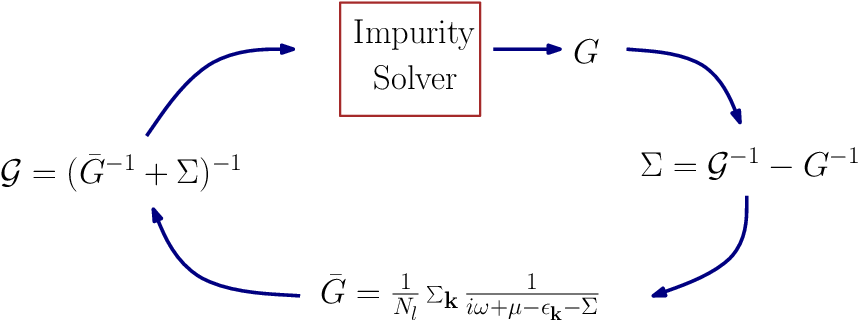
It is usually very difficult to solve lattice models directly due to the exponential increase of the computational costs with the system size because of the interdependent correlations at different length scales. The philosophy behind the DMFT is to treat the local physics numerically exactly, while the non-local fluctuations are treated at a mean-field level. In this way, as showed in Fig. 8, the original lattice system is mapped onto an impurity site embedded in a self-consistently determined effective mean-field medium. This impurity system plus the mean field can be described by the Anderson impurity model, and many numerical methods are available to solve it. Since the mean field needs to be self-consistently determined, an iterative approach is best suited. The algorithm is described in Fig. 9. Note that, as in the main text, we hide the explicit frequency dependence of each quantity to simplify the expressions in the following:
- •
Given the initial impurity self-energy either from perturbation theory or from a previous iteration, we calculate the coarse-grained lattice Green function through
(27) Then the impurity-excluded Green function is calculated by removing the impurity self-energy contribution
(28)
- •
With the calculated impurity-excluded Green function , the impurity problem is well-defined. After the impurity problem is solved, the obtained impurity Green function is used to update the impurity self-energy via the Dyson equation
(29)
These two steps are iterated until the convergence criterion is satisfied.
A.2 Dynamical Cluster Approximation
The DMFT is best suited for studying the local physics, e.g., Mott physics. However, as a single-site approximation it neglects non-local correlations, and hence can not capture the non-local physics, e.g., d-wave superconductivity. To deal with this deficiency of the DMFT, cluster extensions, such as the DCA, have been proposed.
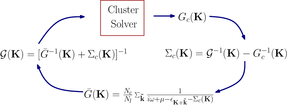
Within the DCA, the original lattice system is mapped onto a periodic cluster (containing multiple sites) instead of an impurity site, embedded in a self-consistently deterrmined mean field. Now, the calculated quantities acquire cluster momentum dependence. As depicted in Fig. 10, the algorithm can be described as:
- •
Given the initial cluster self-energy either from perturbation theory or from a previous iteration, we calculate the coarse-grained lattice Green function through
(30) Then the cluster-excluded Green function is calculated by removing the cluster self-energy contribution
(31)
- •
With the calculated cluster-excluded Green function , the cluster problem is well-defined. It can be solved by different numerical cluster solvers yielding the cluster Green function . The cluster self-energy then can be updated via the Dyson equation
(32)
These two steps are iterated until the convergence criterion is satisfied.
References
- [1] P. Soven, Phys. Rev. 156, 809 (1967).
- [2] R. J. Elliott, J. A. Krumhansl, and P. L. Leath, Rev. Mod. Phys. 46, 465 (1974).
- [3] W. Metzner and D. Vollhardt, Phys. Rev. Lett. 62, 324 (1989).
- [4] E. Müller-Hartmann, Z. Phys. B (Condensed Matter) 74, 507 (1989).
- [5] T. Pruschke, M. Jarrell, and J. Freericks, Advances in Physics 44, 187 (1995).
- [6] A. Georges, G. Kotliar, W. Krauth, and M. J. Rozenberg, Rev. Mod. Phys. 68, 13 (1996).
- [7] M. Hettler, A. Tahvildar-Zadeh, M. Jarrell, T. Pruschke, and H. Krishnamurthy, Phys. Rev. B 58, 7475 (1998).
- [8] M. Hettler, M. Mukherjee, M. Jarrell, and H. Krishnamurthy, Phys. Rev. B 61, 12739 (2000).
- [9] M. Jarrell and H. R. Krishnamurthy, Phys. Rev. B 63, 125102 (2001).
- [10] T. Maier, M. Jarrell, T. Pruschke, and M. H. Hettler, Rev. Mod. Phys. 77, 1027 (2005).
- [11] H. De Raedt and A. Lagendijk, Phys. Rev. Lett. 46, 77 (1981).
- [12] V. Janiš, Phys. Rev. B 64, 115115 (2001).
- [13] A. Toschi, A. A. Katanin, and K. Held, Phys. Rev. B 75, 045118 (2007).
- [14] C. Slezak, M. Jarrell, T. Maier, and J. Deisz, J. Phys.: Condens. Matter 21, 435604 (2009).
- [15] A. N. Rubtsov, M. I. Katsnelson, and A. I. Lichtenstein, Phys. Rev. B 77, 033101 (2008).
- [16] H. Terletska, S.-X. Yang, Z. Y. Meng, J. Moreno, and M. Jarrell, Phys. Rev. B 87, 134208 (2013).
- [17] S.-X. Yang, P. Haase, H. Terletska, Z. Y. Meng, T. Pruschke, J. Moreno, and M. Jarrell, arXiv:1310.6762 (2013).
- [18] H. Hafermann, PhD Thesis, Cuvillier Verlag Goettingen (2010).
- [19] A. Osipov and A. Rubtsov, arXiv:1302.6705 (2013).
- [20] N. E. Bickers, D. J. Scalapino, and S. R. White, Phys. Rev. Lett. 62, 961 (1989).
- [21] C. de Dominicis and P. Martin, J. Math. Phys. 5, 14 (1964).
- [22] S. X. Yang, H. Fotso, J. Liu, T. A. Maier, K. Tomko, E. F. D’Azevedo, R. T. Scalettar, T. Pruschke, and M. Jarrell, Phys. Rev. E 80, 046706 (2009).
- [23] M. Jarrell, T. Maier, C. Huscroft, and S. Moukouri, Phys. Rev. B 64, 195130 (2001).
- [24] P. J. H. Denteneer, R. T. Scalettar, and N. Trivedi, Phys. Rev. Lett. 87, 146401 (2001).
- [25] P. B. Chakraborty, K. Byczuk, and D. Vollhardt, Phys. Rev. B 84, 035121 (2011).
- [26] N. E. Bickers and S. R. White, Phys. Rev. B 43, 8044 (1991).
- [27] H. Hafermann, G. Li, A. N. Rubtsov, M. I. Katsnelson, A. I. Lichtenstein, and H. Monien, Phys. Rev. Lett. 102, 206401 (2009).