Reconstruction of Missing Data using Iterative Harmonic Expansion

Suppose a density fluctuation $\delta(\hat{\mbox{\boldmath$\gamma$}})$ on a unit $N$–sphere $\textrm{S}^{N}$, where $\hat{\mbox{\boldmath$\gamma$}}$ represents a unit vector pointing to a position in $\textrm{S}^{N}$. The masking function is defined by

$\displaystyle\delta_{\rm obs}(\hat{\mbox{\boldmath$\gamma$}})=W(\hat{\mbox{\boldmath$\gamma$}})\delta(\hat{\mbox{\boldmath$\gamma$}}),$

(1)

where $W=0$ inside the masked region and $W=1$ elsewhere. The fluctuation can be expanded in terms of spherical harmonics $X_{i}$,

$\displaystyle\delta(\hat{\mbox{\boldmath$\gamma$}})=\sum_{i}a_{i}X_{i}(\hat{\mbox{\boldmath$\gamma$}}),$

(2)

where $X_{i}(\hat{\mbox{\boldmath$\gamma$}})$ is a solution of the Helmholtz equation, $(\Delta_{N}+k_{i}^{2})X_{i}=0$ where $\Delta_{N}$ is the $N$–dimensional Laplacian on $\textrm{S}^{N}$ and the $k_{i}^{2}$’s are the eigenvalues defined in ascending order $k_{0}^{2}<k_{1}^{2}<k_{2}^{2},\cdots$. We use a single subscript index $i$ to represent the scale of each mode. For instance, for a two–dimensional unit sphere $\textrm{S}^{2}$, the eigenfunction is $Y_{i}$, the spherical harmonics and the eigenvalues are $k_{i}^{2}=\ell(\ell+1)$. The index $i$ of $Y_{i}(\hat{\mbox{\boldmath$\gamma$}})$ is given by a multipole number $l$ and a magnetic quantum number $m$ $i=\ell^{2}+\ell+m+1$.

The sum in Equation (2) should be taken over all $i$–modes. However, in real applications, we can truncate the sum at a certain scale if the modes on smaller scales are not physically relevant. The coefficient $a_{i}$ is called the harmonic coefficient and can be obtained from the inverse transformation of Equation (2). If the fluctuations on the masked region is set to zero, we will obtain the so–called pseudo harmonic coefficients $\tilde{a}_{i}^{\rm P}$s,

$\displaystyle\tilde{a}_{i}^{\rm P}$

$\displaystyle=\int{\rm d}\Omega~\delta(\hat{\mbox{\boldmath$\gamma$}})W(\hat{\mbox{\boldmath$\gamma$}})X^{*}_{i}(\hat{\mbox{\boldmath$\gamma$}})$

(3)

where ${\rm d}\Omega$ is the surface element on $\textrm{S}^{N}$. Equation (3) can be written in terms of the true harmonic coefficients $a_{j}^{\rm true}$s, as

$\displaystyle\tilde{a}_{i}=\sum_{j}~a_{j}^{\rm true}W_{ij},$

(4)

where $W_{ij}$ is the $(i,j)$ component of the mode coupling matrix due to the masking: $W_{ij}=\int{\rm d}\Omega~WX_{j}X_{i}^{*}$.

Equation (4) implies that the true expansion coefficient $\mbox{\boldmath$a$}^{\rm true}$ can be obtained by inverting the mode coupling matrix $W$. However, in general, the matrix can be singular and non–invertible. To regularize a singular matrix, the IHE scheme can be employed. The iteration process starts from a set of the pseudo harmonic coefficients

$\displaystyle\tilde{a}_{i}^{(0)}$

$\displaystyle=\tilde{a}_{i}^{\rm P}.$

(5)

For $n\geq 1$, the $n$–th set of $\tilde{a}_{i}$s can be constructed from two maps: the original map of the unmasked region that was obtained observationally and the map that was reconstructed from the inverse transform of the $n$–th $\tilde{a}_{i}$s in the masked region,

$\displaystyle\tilde{a}_{i}^{(n)}$

$\displaystyle=\int{\rm d}\Omega~\left[\delta(\hat{\mbox{\boldmath$\gamma$}})W(\hat{\mbox{\boldmath$\gamma$}})+\tilde{\delta}^{(n)}(\hat{\mbox{\boldmath$\gamma$}})R(\hat{\mbox{\boldmath$\gamma$}})\right]X_{i}^{*}(\hat{\mbox{\boldmath$\gamma$}}),$

(6)

where

$\displaystyle\tilde{\delta}^{(n)}(\hat{\mbox{\boldmath$\gamma$}})=\sum_{i}^{i_{\rm max}}~\tilde{a}_{i}^{(n-1)}X_{i}(\hat{\mbox{\boldmath$\gamma$}})$

(7)

and $R=1-W$ (see also Fig. 1). Note that the $n$–th iterated real space map contains information equivalent to that conveyed by the $(n-1)$–th harmonic coefficient. Therefore, we call the $\tilde{\delta}^{(N_{\rm I})}$ as the $N_{\rm I}$–th estimator together with $\tilde{a}_{i}^{(N_{\rm I}-1)}$. In the following, we assume that fluctuations whose angular scales are larger than that of the masked region are not significantly correlated with fluctuations smaller than the masked region. In that case, the summations in Eqs. (4) and (7) can be truncated at a certain multipole $i_{\rm max}$, which can be inferred from the size of the mask, as long as we concern large–angle fluctuations corresponding to multipoles $i_{\rm rec,max}\leq i_{\rm max}$. In the following, we sum the $a_{i}$’s up to the multipole $i_{\rm max}$, and we omit the summation symbol when no confusion arises.

Recursively substituting equation (7) into (6), we can obtain the general formula for the $N_{\rm I}$–th iterated harmonic coefficients as a series of $R_{ij}$,

$$\tilde{a}_{i}^{(N_{\rm I}-1)}=\sum_{j}^{i_{\rm max}}\tilde{a}_{j}^{(0)}(\delta^{K}_{ij}+R_{ij}+R^{2}_{ij}+\cdots+[R^{N_{\rm I}-1}]_{ij}),$$

(8)

where $\delta^{K}_{ij}$ is the Kronecker delta, $R_{ij}=\delta^{K}_{ij}-W_{ij}$, and $R^{2}_{ij}=\sum_{k}R_{ik}R_{kj}$ and so on. This finite series, which is truncated at the $N_{\rm I}$–th order represents an asymptotic expansion of $W^{-1}$ in terms of the masked region. As the area of the masked region approaches zero, the series converges to the true value $a_{i}$. As shown in Sec. 2.3, the difference between the $N_{\rm I}$–th estimator and the true $a_{i}$, $\Delta_{i}^{(N_{\rm I}-1)}=|\sum_{j}a_{j}[R^{N_{\rm I}}]_{ij}|$ is of the order of $O(b^{N_{\rm I}})$. Therefore, in the limit of $b\rightarrow 0$, the reconstructed fluctuations converge to the true fluctuations. Even if the area of the mask is finite, the series can converge depending on the following conditions:

• •

  The mask size: As the volume/area of the mask increases, the rate of convergence slows down because the residual matrix $R$ significantly deviates from zero and the contribution to $\Delta_{i}^{(N_{\rm I})}$ is not negligible. We shall discuss this issue in Secs. 2.2 and 2.3.

• •

  The scales we try to reconstruct: The minimum scale corresponding to the highest $i$–mode $i_{\rm rec,max}$ to be reconstructed should be equal to or less than the scale of the $i_{\rm max}$–mode. The choice of the cut–off scale may change the speed of convergence because the mode coupling with the high $i$–modes may become important. We shall discuss this point in Sec. 3.6.

• •

  The spectrum of underlying density fluctuations: If an ensemble averaged density fluctuation has a blue spectrum, the effect of mode coupling, especially from high $i$–modes, becomes more conspicuous than in the cases with red spectra. We shall examine this point in Sec. 3.5.

Therefore, equation (8) can approximate the underlying true density fluctuation. The optimal number of iterations, $N_{\rm I}$, under the given conditions described above should be evaluated using Monte–Carlo simulations; this procedure is discussed later in Sec. 3.

We can think of the reconstruction process as a mapping from an observable to an estimator,

$$F_{\rm IHE}:\tilde{a}_{i}\rightarrow\tilde{a}_{i}^{(N_{\rm I}-1)}.$$

(9)

As we briefly mentioned above and will discuss in more detail in Sec. 3, the accuracy of the IHE method depends on the highest mode to be reconstructed $i_{\rm max}$, the spectrum index $n_{s}$ of the power spectrum of $\delta$, the mask size and the number of total iterations $N_{\rm I}$. Therefore, we can write $F_{\rm IHE}=F_{\rm IHE}(i_{\rm max},n_{s},\mbox{\boldmath$W$},N_{\rm I})$. In Sec. 4.1, we will show that the details of the boundary shape do not significantly affect the reconstruction accuracy if the area of the masked sky is similar.

The IHE method can easily be applied to a sky with an azimuthally symmetric mask. As shown in Fig. 1, the algorithm is simple and easy to implement. The IHE method may also work for three (or higher) dimensional problems provided that the volumes of the missing regions are sufficiently smaller than the scales of interest.

In this section and the next section, we demonstrate that the IHE method gives a finite inversion in the limit that the size of a masked region approaches zero, even in the case when the size is finite. In this section, we consider the reconstruction of the missing fluctuations in a segment on a circle C with a perimeter $L=2\pi$ and show that the IHE method is valid in the limit that the size of the segment converges to zero.

We chose an arbitrary point on C as the origin of the coordinate $\phi$, which runs from -$\pi$ to $\pi$. The mask function is defined as $W(\phi,b)=0$ for $|\phi|<b/2$ and 1 otherwise, where $b$ characterizes the size of the masked region B: $|\phi|<b/2$. Because the eigenfunction $X_{m}$ corresponding to an eigenvalue $k_{m}^{2}=m^{2}$ is given by $\exp(-im\phi)$, a density fluctuation defined on C can be decomposed into discrete Fourier modes as

$\displaystyle\delta(\phi)=\sum_{m=0}a_{m}\exp\left(-im\phi\right),$

(10)

where $m$ is an integer with $m=1$ corresponding to the largest Fourier fluctuation mode on C. As before, the missing fluctuation in the masked region B can be constructed by multiplying the mask function to the original fluctuation: $\delta_{\rm obs}(\phi,b)=\delta(\phi)W(\phi,b)$.

The pseudo–estimator for $\delta$, which is equivalent to the $N_{\rm I}=1$ IHE is given by

$\displaystyle\tilde{\delta}^{(1)}(\phi)=\sum_{m=0}^{m_{\rm max}}\tilde{a}^{(0)}_{m}\exp\left(-im\phi\right),$

(11)

where the Fourier component $\tilde{a}^{(1)}$ is

$\displaystyle\tilde{a}^{(0)}_{m}=\int{\rm d}\phi\delta(\phi)W(\phi,b)\exp\left(im\phi\right).$

(12)

The mask function can be expressed as

$\displaystyle W(\phi,b)=1-\Theta(\phi+b/2)+\Theta(\phi-b/2),$

(13)

where $\Theta(\phi)$ is the Heaviside step function. Then, equation (12) can be rewritten in terms of a true density $a$ as

$\displaystyle\tilde{a}^{(0)}_{m}=\sum_{m^{\prime}}~a_{m^{\prime}}W_{mm^{\prime}},$

(14)

where $W_{mm^{\prime}}=\int{\rm d}\phi W(\phi)\exp[i(m-m^{\prime})\phi]$ corresponds to the mode coupling matrix in equation (4). Explicitly, it can be written as

$\displaystyle W_{mm^{\prime}}=\delta^{K}_{mm^{\prime}}-\frac{2}{m-m^{\prime}}\sin\left[\frac{(m-m^{\prime})b}{2}\right].$

(15)

In the limit of $b\ll 1$, equation (15) can be expanded into a series as

$\displaystyle W_{mm^{\prime}}\simeq\delta^{K}_{mm^{\prime}}-b+\frac{1}{24}(m-m^{\prime})^{2}b^{3}+\cdots.$

(16)

Then, the first iterated IHE estimator is

$\displaystyle\tilde{a}^{(0)}_{m}=a_{m}-\sum_{m^{\prime}}a_{m^{\prime}}\left[b-\frac{1}{24}(m-m^{\prime})^{2}b^{3}+\cdots\right],$

(17)

which will recover the true density fluctuation when $b\rightarrow 0$. In a similar manner, the second iterated estimator can be written as

	$\displaystyle\tilde{a}^{(1)}_{m}$	$\displaystyle=a_{m}-\sum_{m^{\prime}m^{\prime\prime}}a_{m^{\prime\prime}}$
		$\displaystyle\hskip 20.00003pt\times\left[-b^{2}+\frac{(m-m^{\prime})^{2}+(m^{\prime}-m^{\prime\prime})^{2}}{24}b^{4}+\cdots\right].$		(18)

The second iterative estimator also converges to the true density fluctuation in the limit of $b\rightarrow 0$; however, it converges faster than the first iterative estimator because the order of the difference between the estimator and the original value is $b^{2}$ rather than $b$. After $N_{\rm I}$ iterations, we obtain

	$\displaystyle\tilde{a}^{(N_{\rm I}-1)}_{m_{0}}$	$\displaystyle=a_{m_{0}}-\sum_{m_{1}...m_{N_{\rm I}}}a_{m_{N_{\rm I}}}(-b)^{N_{\rm I}-1}$
		$\displaystyle\hskip 20.00003pt\times\left[b-\left.\frac{1}{24}\right\{\left.\sum_{n=1}^{N_{\rm I}}(m_{n-1}-m_{n})^{2}\right\}b^{3}+\cdots\right],$		(19)

where the difference between the $N_{\rm I}$–th estimator and the true fluctuation is of the same order as $b^{N_{\rm I}}$.

In this section, we consider the IHE reconstruction of missing fluctuations on a two dimensional sphere. In what follows, we assume that the mask is azimuthally symmetric: i.e., $W(\hat{\mbox{\boldmath$\gamma$}},b)=0$ for $|\pi/2-\theta|<b$ and 1 otherwise. As described in Sec. 2.2, the pseudo– or first IHE estimator can be written as,

	$\displaystyle a^{(0)}_{i}$	$\displaystyle=\int\!\!{\rm d}\Omega~\delta(\hat{\mbox{\boldmath$\gamma$}})W(\hat{\mbox{\boldmath$\gamma$}},b)Y_{i}(\hat{\mbox{\boldmath$\gamma$}})$		(20)
		$\displaystyle=a_{i}-\int\!\!{\rm d}\Omega~\delta(\hat{\mbox{\boldmath$\gamma$}})R(\hat{\mbox{\boldmath$\gamma$}},b)Y_{i}(\hat{\mbox{\boldmath$\gamma$}}).$		(21)

Note that we have written equation (21) in terms of $R=1-W$ rather than $W$ to limit the integral range to the vicinity of $\theta\sim\pi/2$, which facilitates analysis of the behavior of the estimator. Note also that the subscript $i$ denotes a set of parameters $\ell$ and $m$. Using equations (4) and (5), we can write equations (20) and (21) as

$\displaystyle a_{i}^{(0)}=a_{i}-\sum_{j}a_{j}R_{ij}$

(22)

where $R_{ij}$ is the residual mask matrix,

$\displaystyle R_{i_{1}i_{2}}=\sum_{i_{3}}s_{i_{3}}T_{i_{1}i_{2}i_{3}},$

(23)

and $s_{i}$ denotes the harmonic expansion of the mask residual, $s_{i}=\int{\rm d}\Omega R(\hat{\mbox{\boldmath$\gamma$}},b)Y_{i}^{*}(\hat{\mbox{\boldmath$\gamma$}})$. The matrix $T$ is explicitly given in Hivon et al. (2002) as

	$\displaystyle T_{i_{1}i_{2}i_{3}}$	$\displaystyle=\int\!{\rm d}\Omega~Y_{i_{3}}Y_{i_{2}}^{*}Y_{i_{1}}$
		$\displaystyle=(-1)^{m_{2}}\left[\frac{(2\ell_{1}+1)(2\ell_{2}+1)(2\ell_{3}+1)}{4\pi}\right]^{1/2}$
		$\displaystyle\hskip 14.22636pt\times\left(\begin{array}[]{ccc}\ell_{1}&\ell_{2}&\ell_{3}\\ 0&0&0\end{array}\right)\left(\begin{array}[]{ccc}\ell_{1}&\ell_{2}&\ell_{3}\\ m_{1}&-m_{2}&m_{3}\end{array}\right),$

where $(:::)$ is the Wigner 3$j$–symbol. Note that the subscript $i_{j}$ depends only on $\ell_{j}$ and $m_{j}$, i.e. $i_{j}=\ell_{j}^{2}+\ell_{j}+m_{j}+1$.

For an azimuthally symmetric mask, $s_{i}$ can be analytically integrated and expanded in terms of $b(\ll 1)$ as

	$\displaystyle s_{i}$	$\displaystyle=\int_{0}^{2\pi}\!\!d\phi\int_{\pi/2-b}^{\pi/2+b}\!\!d\cos\theta~Y_{i}(\theta,\phi=0)$
		$\displaystyle=2\pi\sqrt{\frac{(2\ell+1)\cos^{2}(b)}{4\pi}}\frac{P_{\ell 1}[\sin(b)]-P_{\ell 1}[\sin(-b)]}{\ell(\ell+1)}$		(28)
		$\displaystyle\simeq c_{i}^{(1)}b+c_{i}^{(3)}b^{3}+{\mathcal{O}}[b^{4}],$		(29)

where the explicit form of the $c_{i}$’s is given by

	$\displaystyle c_{i}^{(1)}$	$\displaystyle=2\sqrt{(2\ell+1)\pi}P_{\ell 0}(0),$		(30)
	$\displaystyle c_{i}^{(3)}$	$\displaystyle=-\frac{1}{3}\sqrt{(2\ell+1)\pi}[P_{\ell 0}(0)-P_{\ell 2}(0)],$		(31)

where $P_{\ell m}$ is the associated Legendre function. Because $s_{i}$ is the first order of $b$ and the matrix $R_{ij}$ is a linear combination of the $s_{i}$s, the lowest order of $R_{ij}$ is $b$. Therefore, the leading order of the difference between the first IHE estimator and the true fluctuation, $\Delta^{(0)}_{i}\equiv|a_{i}^{(0)}-a_{i}|$, is also $b$. For the second iterated IHE estimator, we have

$\displaystyle a^{(1)}_{i}=a_{i}-\sum_{j,k}a_{k}R_{kj}R_{ji},$

(32)

and, therefore, $\Delta^{(1)}_{i}=O(b^{2})$. As in the one–dimensional case, for a given $N_{\rm I}$, we expect that, $\Delta^{(N_{\rm I}-1)}_{i}=O(b^{N_{\rm I}})$. However, note that $\Delta^{(N_{\rm I})}_{i}$ scales to $0$ as $b\rightarrow 0$ but does not approach $0$ as $N_{\rm I}\rightarrow\infty$ due to the mode coupling between the different multipole modes, as shown in equation (19). Instead, it converges to the one for the direct inversion as illustrated later in Fig. 3.

Fig. 2 presents the $D^{2}$ accuracy of the IHE map reconstruction as a function of the angular size of the masked region, which is compared to the accuracy of the truncated asymptotic expansion in equation (22). To compute the $D^{2}$ accuracies we used the fiducial set of simulations described in Section 3.1 with various mask sizes. The circles and diamonds represent the $D^{2}$ accuracies defined by equation (33) for the IHE reconstruction and the truncated asymptotic expansion defined by equation (22), respectively with filled symbols denoting 1 iteration and open symbols corresponding to 4 iterations. One can see that the filled and open circles and diamonds agree very well, suggesting that the convergence of the IHE method can be numerically verified. Furthermore, we expect from equation (32) that the $D^{2}$ accuracy improves as the number of iterations increases. This tendency is more clearly observable at smaller $b$. In the following, we discuss the reconstruction of the missing fluctuations on a two–dimensional sphere;however, in general, the reconstruction method can be used for an $N$–dimensional sphere.

To assess the reconstruction accuracy, we generated $10^{3}$ random realisations of an isotropic Gaussian density field in the sky. We used the code synfast, which is publicly available as a package in HEALPIX to generate random Gaussian maps. First, we used the Harrison–Zel’dovich spectrum as the input power spectrum. It gives an angular power spectrum $C_{\ell}\propto\ell^{n_{s}}$, where $n_{s}=-2$ on large angular scales, in the Einstein de–Sitter universe, which corresponds to the Sachs–Wolfe plateau of the CMB power spectrum. We set the monopole power to zero because it is a uniform value over the unmasked sky and can be subtracted out before reconstruction. As a simple model of the zone of avoidance, we considered an azimuthally symmetric mask with $W(\hat{\mbox{\boldmath$\gamma$}})=0$ at $|\pi/2-\theta|<b$ and $W=1$ otherwise with $b=20^{\circ}$. We used pixels that were sufficiently smaller than the size of the mask and the reconstructed fluctuation scales to reduce errors due to the pixelization effect. We adopt the Healpix resolution $N_{\textrm{side}}=1024$ (the total number of pixels in the entire sky is $N_{\textrm{pix}}=12\times N_{\textrm{side}}^{2}\simeq 1.2\times 10^{7}$), where the pixel size corresponds to $3.4$ arcmin. The input power spectrum should be truncated at scales $\ell_{\rm cut}$ sufficiently small compared to the reconstructed scales $\ell_{\rm max}$, i.e. $\ell_{\rm max}\ll\ell_{\rm cut}$. In our simulated maps, we set $\ell_{\rm cut}=30$, which is a scale sufficiently smaller than the mask size. We also conducted the same analysis with $\ell_{\rm cut}=100$; however, the result was unchanged. We use this set of fiducial simulations unless otherwise stated. In addition to this fiducial set, we also generated the same simulation set for the input spectrum indices $n_{s}=0$ and $n_{s}=-4$.

The deviation from the original fluctuations can be measured from the ratio of the L² norms denoted by $D^{2}$,i.e. the squared difference between the density fluctuations of the original and reconstructed maps divided by the squared density fluctuations of the original map:

$\displaystyle D^{2}\equiv\frac{\sum_{i}^{N{\rm pix}}[\delta_{\rm rec}(\hat{\mbox{\boldmath$\gamma$}}_{i})-\delta_{\rm true}(\hat{\mbox{\boldmath$\gamma$}}_{i})]^{2}}{\sum_{i}^{N{\rm pix}}\delta_{\rm true}^{2}(\hat{\mbox{\boldmath$\gamma$}}_{i})}$

(33)

where $\delta_{\rm rec}$ and $\delta_{\rm true}$ describe the reconstructed and the original density fluctuations up to the highest multipole:

	$\displaystyle\delta_{\rm true}(\hat{\mbox{\boldmath$\gamma$}})$	$\displaystyle\equiv\sum_{i=0}^{i_{\rm rec,max}}a_{i}^{\rm true}Y_{i}(\hat{\mbox{\boldmath$\gamma$}}),$		(34)
	$\displaystyle\delta_{\rm rec}(\hat{\mbox{\boldmath$\gamma$}})$	$\displaystyle\equiv\sum_{i=0}^{i_{\rm rec,max}}a_{i}^{(N_{\rm I})}Y_{i}(\hat{\mbox{\boldmath$\gamma$}}).$		(35)

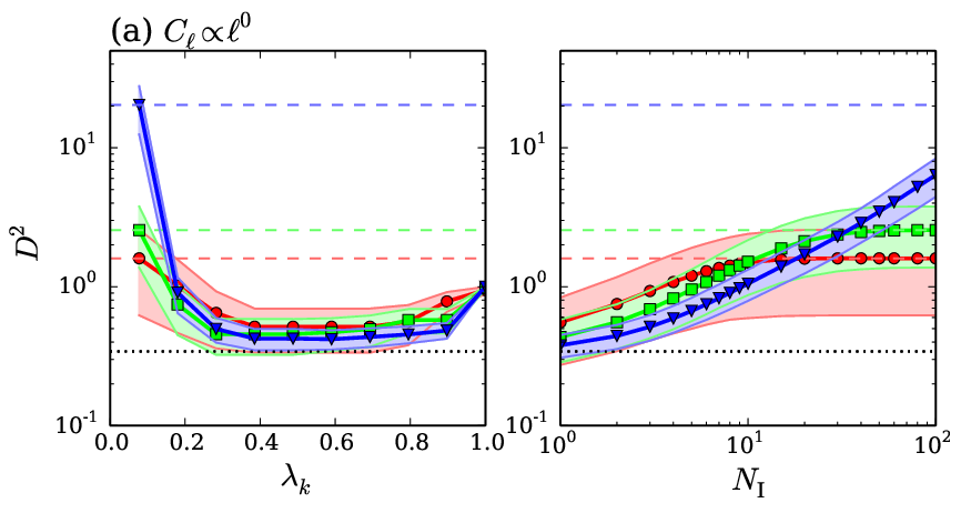
Using equation (4), we can compare the IHE method to the brute–force inversion of the matrix $W$ and the SVD (Efstathiou, 2004). If the mode coupling matrix $W$ is invertible, we obtain a unique solution for the underlying density fluctuation within the mask. However, if the matrix $W$ contains some eigenvalues that are close to zero, where the matrix is close to being singular, the inversion causes large errors. In such cases, we can remove the singularities by replacing the small eigenvalues with zero; this procedure is called the SVD method. Note that the order of the matrix $W$ is closely related to the singularity of $W$. If we take the order of $W$ to be sufficiently large to include most of the modes that are coupled to $a_{i}$, the inverse of $W$, if it exists, gives an accurate solution of $a_{i}$. However, the matrix inversion is hampered by the ill-posed nature of the inversion due to singularities. Conversely, if we truncate the order of $W$ at a sufficiently small scale $\ell_{\rm max}$, the matrix is invertible; however, the inversion matrix gives a biased solution of $a_{i}$ because the possible couplings from higher modes are discarded by the $\ell_{\rm max}$ truncation. Here we define $W$ as an $i_{\rm max}\times i_{\rm max}$ matrix. As the first step of the SVD method, we decompose the matrix $W$ into three matrices:

$$\mbox{\boldmath$W$}=\mbox{\boldmath$U$}~\mbox{\boldmath$\Sigma$}~\mbox{\boldmath$V$}^{\dagger},$$

(36)

where $V$ and $U$ are $i_{\rm max}\times i_{\rm max}$ unitary matrices and the superscript $\dagger$ denotes the Hermitian conjugate. $\Sigma$ is the diagonal matrix, which consists of the eigenvalues of $W$, called the singular values. The order of the eigenvalues in $\Sigma$ is arbitrary; however, they are arranged in a descending order so that the decomposition is determined uniquely. Let the $k$–th eigenvalue be $\lambda_{k}$, and the eigenvalues smaller than $\lambda_{k}$ be zero. Then, the pseudo–inversion of $W$ can be written in terms of $\Sigma^{+}$, the rank–$k$ diagonal matrix that consists of the reciprocal of the non–zero eigenvalues that are equal to or larger than $\lambda_{k}$:

$$\mbox{\boldmath$W$}^{+}=\mbox{\boldmath$V$}~\mbox{\boldmath$\Sigma$}^{+}~\mbox{\boldmath$U$}^{\dagger},$$

(37)

which gives

$$a^{\rm est}_{i}=\sum_{j}\tilde{a}_{j}W^{+}_{ij}.$$

(38)

The choice of the threshold $\lambda_{k}$ is not trivial and should be carefully determined a priori because the mapping $F_{\rm SVD}$ depends on various factors including the threshold $\lambda_{k}$, i.e. $F_{\rm SVD}=F_{\rm SVD}(\ell_{\rm max},n_{s},{\boldsymbol{W}},\lambda_{k})$. In this context, a singularity can only be defined in terms of $\lambda_{k}$. More specifically, the mapping $F_{\rm SVD}$ is contaminated by the eigenvalues that are close to being singular if $\partial D^{2}/\partial\lambda_{k}<0$. In such cases, the threshold of the eigenvalues should be increased to enable more accurate reconstruction. The brute–force inversion corresponds to $F_{\rm inv}=F_{\rm SVD}(\ell_{\rm max},n_{s},{\boldsymbol{W}},\lambda_{k}=0)$. The optimal choice of $\ell_{\rm max}$ should depend on $n_{s}$, $W$ and even on $\ell_{\rm rec,max}$. Here we simply set $\ell_{\rm max}=\ell_{\rm rec,max}$.

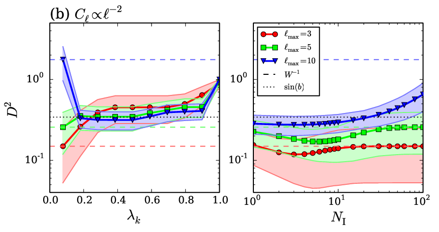
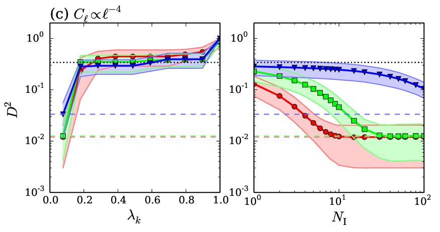
In the left panels of Fig. 3, $D^{2}$ is depicted as a function of the minimum non–zero eigenvalue $\lambda_{k}$. The solid lines represent the different maximum multipoles to be reconstructed, $\ell_{\rm max}=3,5$ and $10$. The three different rows show the different input power spectra, which will be discussed in detail in Sec. 3.5. Let us focus on the middle left panel. For $\ell_{\rm max}=3$ and $5$, $D^{2}$ increases monotonically as the threshold increases. Thus, $F_{\rm SVD}$ is not contaminated by singular eigenvalues because $\partial D^{2}/\partial\lambda_{k}>0$. On the other hand, Conversely, for $\ell_{\rm max}=10$, $D^{2}$ has a minimum near $\lambda_{k}\sim 0.4$. Therefore, eigenvalues smaller than $\sim 0.4$ may be the contaminants of the mapping $F$, and we can better estimate the original density fluctuations when we limit the eigenvalues to $\lambda<0.4$. In the right panel of Fig. 3, we show $D^{2}$ for the IHE method as a function of the number of iterations. The $D^{2}$ has a minimum near $N_{\rm I}<10$ that depends on the maximum multipole. After a sufficient number of iterations, $D^{2}$ converges to the brute–force inversion results, which are shown as the horizontal dashed lines in Fig. 3, i.e. $F_{\rm IHE}(N_{\rm I}\rightarrow\infty)=F_{\rm inv}$. The IHE method with a certain finite number of iterations is therefore always more accurate than the SVD method. However, in practice, we should know the optimal number of iterations a priori. This number depends on the mask size, the maximum multipole to be reconstructed and the underlying spectrum of the density fluctuation. We can estimate the optimal iteration number using Monte–Carlo simulations. In Sec. 3.5 we will see how the result changes for different types of underlying power spectra.

Note that the computation time for estimating $\tilde{a}^{(N_{\rm I})}$ can be significantly reduced if we use equation (6) instead of equation (8). The reason is as follows. Because the rank of the matrix $R_{ij}$ is on the order of $\ell_{\rm max}^{2}$, it costs $N_{\rm pix}\ell_{\rm max}^{4}$ according to equation (2.3), and the matrix algebra of equation (8) costs $\sim N_{\rm I}\ell_{\rm max}^{6}$ computations. If one uses (equation (6), it would be on the order of $N_{\rm I}N_{\rm pix}\ell_{\rm max}^{2}$, where $N_{\rm I}$ is the number of iterations, $N_{\rm pix}$ is the number of pixels that tile the sky and $\ell_{\rm max}$ is the maximum multipole to be reconstructed. For example, for given $\ell_{\rm max}=10$, $N_{\rm pix}=12\times 1024^{2}$ pixels and five iterations, the computation time will be reduced by a factor of $\sim 25$.

The statistical isotropy of the CMB map (Planck Collaboration, 2015c, e.g.) and its Gaussianity (Planck Collaboration, 2015d, e.g.) has previously been examined. When the map reconstruction method is applied to the CMB map, the statistical properties of the CMB temperature fluctuations should remain unchanged. Using our fiducial simulation set ($n_{s}=-2,\ell_{\rm rec,max}=5$ and $b=20^{\circ}$), which is described in Sec. 3.1, we discuss how the IHE method affects the underlying statistical properties via the reconstruction.

In Sec. 3.3.2, we demonstrated that the IHE reconstruction does not significantly change the statistical properties of the map. In this section, we will show how a two-point statistic, the power spectrum, is affected or recovered using the IHE method. Again, we use our fiducial simulation set to access the reconstruction. The power spectrum of the $\alpha$-th realization map can be estimated to be

$\displaystyle\hat{C}_{\ell}^{\alpha}=\frac{1}{2\ell+1}\sum_{m}\left|a_{\ell m}^{\alpha}\right|^{2},$

(46)

where the true power spectrum can be estimated from the arithmetic mean over 1000 realizations, $C_{\ell}=\langle\hat{C}_{\ell}\rangle=\sum_{\alpha}\hat{C_{\ell}^{\alpha}}/1000$ with a variance of $\sigma^{2}_{\ell}=\sum_{\alpha}(\hat{C}_{\ell}^{\alpha}-C_{\ell})^{2}/999$. To quantify the discrepancy between the power spectra of the reconstructed and original fluctuations, we use the relative difference summed over the multipoles,

$\displaystyle\delta C=\sum_{\ell}\left(\frac{C^{\rm rec}_{\ell}}{C^{\rm org}_{\ell}}-1\right),$

(47)

and the Maharanobis distance,

$\displaystyle D_{\rm M}^{2}=\sum_{\ell}^{\ell_{\rm rec,max}}\frac{(C_{\ell}^{\rm rec}-C_{\ell}^{\rm org})^{2}}{\sigma_{\ell}^{2}},$

(48)

where $C_{\ell}^{\rm rec}$ is estimated from either a pseudo-fluctuation or the IHE reconstructed fluctuations. Fig. 5 shows the averaged power spectrum of the fiducial simulations normalized by input spectrum. We obtained $\delta C=-0.29$ and $0.022$ for the pseudo- and IHE reconstructions and found that for $\ell\leq 5$, $D^{2}_{\rm M}=0.88$ and $0.48$, respectively. Therefore, the IHE method provides a less biased estimate of the power spectrum $C_{\ell}$. On large scales, the suppression of the power due to the masking is mitigated by the IHE reconstruction, while on smaller scales, $\ell\simeq\ell_{\rm rec,max}$ and the reconstruction slightly overestimates the power spectrum.

The reconstruction accuracy depends on the underlying power spectrum $C_{\ell}\propto\ell^{n_{s}}$ of the fluctuation because the harmonic modes are not independent in the masked incomplete sky even if the underlying fluctuation is Gaussian. We consider three power law indices, $n_{s}=0,-2$ and $-4$, which correspond to the following three cases. The projected two-dimensional galaxy or dark matter distribution is approximated as $C_{\ell}^{\rm g}\propto\ell^{0}$ (Frith et al., 2005, e.g.) on large scales, and the ordinary Sachs–Wolfe spectrum is approximated as $C_{\ell}^{\rm SW}\propto\ell^{-2}$ (Sachs & Wolfe, 1967). On very large–angular scales, the integrated Sachs–Wolfe effect, which gives $C_{\ell}^{\rm ISW}\propto\ell^{-4}$ (Cooray, 2002, e.g.) dominates the CMB in the standard $\Lambda$CDM scenario.

Given the typical scale of the mask $\theta_{\rm M}$, it is impossible to reconstruct a fluctuation whose scale is smaller than $\ell_{\rm max}\simeq\ell_{\rm M}\geq 180/\theta_{\rm M}$. Due to the mode coupling, fluctuations with angular scales corresponding to $\ell_{\rm M}$ are strongly affected by fluctuations with smaller angular sizes. If the spectral index is negative, the amplitude of a smaller scale fluctuation is weak and does not strongly disturb the large-scale fluctuations. Therefore, the deconvolution mapping $F$ is less affected by singularities. However, if the spectrum is flat or has a positive slope, the large-scale modes are highly contaminated by the small-scale fluctuations.

In Fig. 3, the top and bottom panels show the $D^{2}$ accuracies for $n_{s}=0$ and $n_{s}=-4$. For the $n_{s}=0$ case, the SVD has a minimum at $\lambda_{k}\sim 0.5$ that is larger than when $n_{s}=-2$. Thus, $F_{\rm SVD}(n_{s}=0)$ is more affected by singularities than $F_{\rm SVD}(n_{s}=-2)$. The IHE results in the right panels shows that $N_{\rm I}=1$ gives the highest accuracy and that the reconstructed accuracies gradually degrade to the value given by the brute–force method. Conversely, $F_{\rm SVD}(n_{s}=-4)$ is not affected by singularities because it always shows $\partial D^{2}/\partial\lambda_{k}<0$ for the SVD method.

It is important to pay attention to the dependence of the reconstruction accuracy on the multipoles $\ell$ and $m$. If there are particular modes that do not suffer from the masking effect, we can use them to perform robust cosmological analysis.

Fig. 6 shows a scatter plot of the original and reconstructed $a_{\ell m}$s for an azimuthally symmetric $\pm 20^{\circ}$ mask. The solid line represents a relation in which the reconstructed $a_{\ell m}$ is identical to the original one. The dashed red and blue lines in each panel are the best linear fits for the pseudo–$a_{\ell m}$s and the IHE method, respectively. The statistical accuracy is also shown in each panel: $\delta$, $\sigma$ and $r$ are the average differences between the original and reconstructed $a_{\ell m}$s, the standard deviation, and the best fitted slope of the linear fit, respectively. We note the following three characteristics:

• •

  For the odd modes ($\ell+m=2n+1$, where $n$ is an integer), the masking effect is sufficiently small to enable accurate map reconstruction. In that case, the pseudo–$a_{\ell m}$’s are already accurate and the IHE method slightly improves the accuracy.

• •

  For the even modes ($\ell+m=2n$, where $n$ is an integer), the masking systematically suppresses the amplitude of fluctuations. For a given $\ell$ mode, the suppression is more significant for larger $m$ modes.

• •

  For a given $\ell$ mode, the masking effect is the most significant for the $\ell=m$ mode and the effect is more significant for higher $\ell$ modes.

These dependencies are closely related to the value of the diagonal part of the mask matrix, i.e.

$$Q_{\ell m}\equiv W_{\ell m\ell m}=\int\!{\rm d}\cos\theta{\rm d}\phi\left|Y_{\ell m}(\theta,\phi)\right|^{2}W(\theta,b),$$

(49)

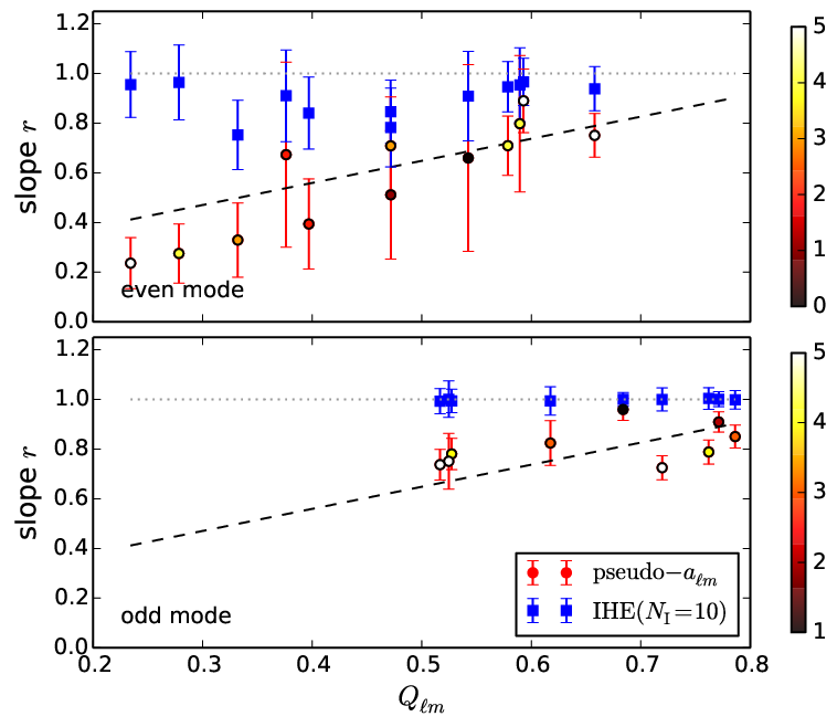
which quantifies how important the fluctuation outside the masked region is and takes values between 0 and 1. In the limit where the area of the masked region approaches zero, the mask matrix becomes an identity matrix; therefore, $Q_{\ell m}\rightarrow 1$, which means that $100\%$ of the fluctuation distribution is outside the mask. For the odd modes, because $Y_{\ell m}$ is small near the equator, i.e. within the masked region, the fluctuation in the masked region is not significantly different from zero. In this case, $Q_{\ell m}$ is close to unity. Conversely, for the even modes, $Y_{\ell m}$ takes relatively larger values near the equator; therefore, the fluctuation inside the mask becomes important compared to that outside the mask. In this case, $Q_{\ell m}$ is close to zero. Therefore, the above dependency of the reconstruction accuracy is simply correlated with the choice of the basis function relative to the mask geometry. The circle symbols in Fig. 7 show the best fit of the slope of the pseudo–$a_{\ell m}$s obtained in Fig. 6 as a function of $Q_{\ell m}$ for the even (top–panel) and odd (bottom–panel) modes, respectively. We can see a clear correlation between the slopes and $Q_{\ell m}$s. For the odd modes, the $Q_{\ell m}$s are larger, while they are smaller for the even modes. In each panel, the different $\ell$ modes are distinguished by the color levels. It is evident that the lower $\ell$ modes tend to have a larger values of $Q_{\ell m}$ and, therefore, larger slopes $r$. The blue squares in Fig. 7 are the same as before but for the $a_{\ell m}$ reconstructed using the IHE method. Note that the IHE reconstruction works pretty well for the odd modes, as the slope $r\sim 1$ implies. Conversely, the reconstruction for the even modes is less accurate than that for the odd modes.

Even though $Q_{\ell m}$ can explain the strength of suppression of the $a_{\ell m}$s, it does not have a perfect correlation with the slope $r$. Consequently, we need to consider other factors as well. As we mentioned above, $Q_{\ell m}$ represents the amount of fluctuations leaking outside the masked region. In other words, $Q_{\ell m}$ represents a fraction of the diagonal components in the mode coupling matrix $W_{\ell m\ell^{\prime}m}$, where $\sum_{\ell^{\prime}}W_{\ell m\ell^{\prime}m}=1$ for a given $\ell$ and $m$ mode. Note that for azimuthally symmetric masks, the $W_{\ell m\ell^{\prime}m^{\prime}}$s have non–zero values only for the $m=m^{\prime}$ and $\ell^{\prime}=\ell+2n$ modes, where $n=0,1,2,\cdots$. Fig. 8 shows the non–zero components of the mask matrix, $W_{\ell m\ell^{\prime}m}$. The top and bottom panels show the $\ell=m$ modes for different $\ell$ and the different $m$ modes for $\ell=5$, respectively. In the top panel, it is evident that $W$ at $\ell^{\prime}=m$, which is $Q_{\ell m}$, decreases monotonically with $\ell^{\prime}$. It is also apparent that for the $b=\pm 1^{\circ}$ case, the matrix is almost diagonal, while for the $b=\pm 20^{\circ}$ case, there is a long tail towards higher $\ell$ modes. This tail can induce mode coupling between different $\ell$ modes, and the strength of the coupling depends on each realisation of the map. The scattering of points centered at the dashed lines in Fig. 7 may be due to this effect.

We again consider an isotropic Gaussian prior; however, now, we discuss the application of the IHE method to more realistic cases. First, we describe a reconstruction of the CMB map, which is masked by the Galactic plane. In the concordant model, on superhorizon scales, the spectral index of the CMB power spectrum is approximately given by $n_{s}=-4$ because the ISW effect is dominant. On horizon scales, the index increases to $n_{s}=-2$, which corresponds to the Harrison-Zel’dovich spectrum because the ordinary Sachs-Wolfe effect is dominant. On subhorizon scales, the index increases to $n_{s}\simeq-1$ if the scale is smaller than the sound horizon at the last scattering time.

In this study, we used the Galactic masks provided by the Planck DR2 ²² 2 http://irsa.ipac.caltech.edu/data/Planck/release_2/ancillary-data/ (Planck Collaboration, 2015a), and neglected the point source masks because the masks for each point source were too small to affect the reconstruction of the large mode fluctuations, $\ell<10$. However, note that the fluctuations inside the point source mask could be well reconstructed by limiting the reconstruction area in the vicinity of the point source mask region instead of the entire sky. In that case, we could redefine a local orthogonal system, i.e. the harmonics in the finite two-dimensional flat space. However, such analysis was beyond the scope of this study and will be investigated in the future. Figure 9 illustrates the Galactic masks we used. The colors (from black to white) show different masking schemes in which the areas of the unmasked regions are $60\%,70\%,80\%,90\%$ and $97$ % of the entire sky. We generated 1000 random Gaussian simulations with an input spectrum from the latest Planck $\Lambda$CDM cosmological model Planck Collaboration (2015b).

Figure 10 presents the reconstruction accuracy for the simulated CMB maps masked by the Galactic plane. For all the $\ell_{\rm rec,max}$, the IHE reconstruction with a finite number of iterations gives better reconstructions than the direct inversion. By comparing the results with those shown in Figure 3, remembering that $65$% of the sky of a $b=20$ mask is unmasked, it can be seen that the $n_{s}=-2$ results are consistent with the case in which the Galactic plane is masked. As mentioned, the detailed shape of the mask does not significantly affect the reconstruction using the IHE method if the area of the masked sky is similar. The optimal number of iterations depends on the size of the mask and the reconstruction scale $\ell_{\rm rec,max}$; therefore, the number of iterations should be determined before reconstructing the CMB map.

In the past sections, we demonstrated that the IHE reconstruction method could be applied to Gaussian isotropic fluctuations. In practice, the map may contain non-Gaussian features. In this section, we consider two types of non-Gaussian priors. First, we consider a type of isotropic non-Gaussian fluctuation induced by primordial non-Gaussianity in the density perturbation. The local type non-Gaussianity on large-scale CMB fluctuations can be written as,

$$\frac{\Delta T}{T}=\left(\frac{\Delta T}{T}\right)_{\rm G}-3f_{\rm NL}\left\{\left(\frac{\Delta T}{T}\right)_{\rm G}^{2}-\left\langle\left(\frac{\Delta T}{T}\right)_{\rm G}^{2}\right\rangle\right\},$$

(50)

where $\langle\Delta T/T\rangle_{\rm G}$ is a Gaussian fluctuation of the CMB temperature in the sky. The map is scaled to its root mean square to be $\langle\Delta T/T\rangle_{\rm G}=10^{-4}$ so that readers can compare the value of the $f_{\rm NL}$ to the one introduced in the CMB analysis. We show the reconstruction accuracies for $f_{\rm NL}=0$ and $5000$ for comparison. Given that the recent CMB observation by Planck suggest that the value of $f_{\rm NL}$ is consistent with zero (Planck Collaboration, 2015d), the value of $f_{\rm NL}=5000$ assumed here might be too large. However, even in such an extreme case of non-Gaussianity, we found that the IHE reconstruction accuracy was not affected much. Here, we fixed the azimuthal mask size to $b=20^{\circ}$ as before.

Figure 11 shows the map reconstruction accuracies as a function of the number of iterations for IHE. The results are compared with the isotropic Gaussian prior case. It is evident that even if the non-Gaussianity is quite large, such as $f_{\rm NL}=5000$, the reconstruction accuracy does not significantly change compared to the isotropic Gaussian prior case. This result implies that the IHE method is robust against the probability distribution of the underlying fluctuation as long as the statistical isotropy holds.

Second, we consider an anisotropic non-Gaussian prior. For instance, if there is a large non-Gaussian structure in the universe, it can affect the CMB sky via the ISW effect. To simulate this situation, we first generated a Gaussian isotropic map and then added a circular structure that had a Gaussian radial profile:

$$\frac{\Delta T}{T}(\hat{\mbox{\boldmath$n$}})=\left(\frac{\Delta T}{T}\right)_{\rm G}(\hat{\mbox{\boldmath$n$}})+A^{\prime}_{\sigma}\exp\left[\frac{(\hat{\mbox{\boldmath$n$}}-\hat{\mbox{\boldmath$n$}}_{0})^{2}}{2r_{\sigma}^{2}}\right],$$

(51)

where $A^{\prime}_{\sigma},r_{\sigma}$ and $\hat{\mbox{\boldmath$n$}}_{0}=(\theta_{0},\phi_{0})$ are free parameters that specify the amplitude, size and the center position of a non-Gaussian structure. $A^{\prime}_{\sigma}$ is the amplitude of a circular symmetric non-Gaussian structure with a Gaussian profile with a radius $r_{\sigma}$.

It is more convenient to rewrite the parameter as $A^{\prime}_{\sigma}=A_{\sigma}\ell(\ell+1)C_{\ell}/2\pi$, where $\ell=\pi/r_{\sigma}$. We chose to use $A_{\sigma}=1$ and $10$ and $r_{\sigma}=10^{\circ}$ and $40^{\circ}$ in this study. Note that the azimuthal position of the structure $\phi_{0}$ does not affect the results because the background Gaussian field is statistically isotropic and the mask we considered is independent of the azimuthal position. Therefore, we can always set $\phi_{0}=0$ without losing generality. $\theta_{0}$ was chosen such that the center of structure would correspond to the center of the mask ($\theta_{0}=90[\textrm{deg}]$), the edge of the mask ($\theta_{0}=70[\textrm{deg}]$), and completely outside the mask ($\theta_{0}=0$).

Figures 12-14 show the map reconstruction accuracies as a function of the number of iterations for background fluctuations with power-law indices $n_{s}=0,-2$ and $-4$. For the $n_{s}=-2$ and $-4$ backgrounds, the effect of the non-Gaussian structure is very small, while for $n_{s}=0$ background, the effect is prominent. We obtained higher reconstruction accuracies for larger structures. Therefore, adding a structure with $r_{\sigma}$ increases the amplitude of the power spectrum at $\ell\simeq\pi/r_{\sigma}$, e.g. $\ell\sim 3$ for $r_{\sigma}=40^{\circ}$. For the $n_{s}=0$ spectrum, adding power to large scales may greatly change the effective slope of the spectrum so that the spectrum becomes redder, which acts to mitigate the mode–mode coupling. However, further studies are necessary to examine the reason for this phenomenon.

References

- Abramo et al. (2006) Abramo L. R., Sodré, Jr. L., Wuensche C. A., 2006, Phys. Rev. D, 74, 083515
- Abrial et al. (2008) Abrial P., Moudden Y., Starck J.-L., Fadili J., Delabrouille J., Nguyen M. K., 2008, Statistical Methodology, 5, 289
- Afshordi et al. (2009) Afshordi N., Geshnizjani G., Khoury J., 2009, JCAP, 8, 30
- Aurich et al. (2010) Aurich R., Lustig S., Steiner F., 2010, Classical and Quantum Gravity, 27, 095009
- Aurich et al. (2007) Aurich R., Lustig S., Steiner F., Then H., 2007, Classical and Quantum Gravity, 24, 1879
- Bennett et al. (2011) Bennett C. L. et al., 2011, ApJS, 192, 17
- Bernui & Hipólito-Ricaldi (2008) Bernui A., Hipólito-Ricaldi W. S., 2008, MNRAS, 389, 1453
- Bernui et al. (2006) Bernui A., Villela T., Wuensche C. A., Leonardi R., Ferreira I., 2006, Astronomy & Astrophysics, 454, 409
- Bucher & Louis (2012) Bucher M., Louis T., 2012, MNRAS, 424, 1694
- Cooray (2002) Cooray A., 2002, Phys. Rev. D, 65, 083518
- Copi et al. (2007) Copi C. J., Huterer D., Schwarz D. J., Starkman G. D., 2007, Phys. Rev. D, 75, 023507
- Cruz et al. (2008) Cruz M., Martínez-González E., Vielva P., Diego J. M., Hobson M., Turok N., 2008, MNRAS, 390, 913
- Cruz et al. (2011) Cruz M., Vielva P., Martínez-González E., Barreiro R. B., 2011, MNRAS, 412, 2383
- de Oliveira-Costa et al. (2004) de Oliveira-Costa A., Tegmark M., Zaldarriaga M., Hamilton A., 2004, Phys. Rev. D, 69, 063516
- Efstathiou (2004) Efstathiou G., 2004, MNRAS, 348, 885
- Efstathiou et al. (2010) Efstathiou G., Ma Y.-Z., Hanson D., 2010, MNRAS, 407, 2530
- Emir Gümrükçüoglu et al. (2007) Emir Gümrükçüoglu A., Contaldi C. R., Peloso M., 2007, JCAP, 11, 5
- Eriksen et al. (2007) Eriksen H. K., Banday A. J., Górski K. M., Hansen F. K., Lilje P. B., 2007, ApJL, 660, L81
- Fialkov et al. (2010) Fialkov A., Itzhaki N., Kovetz E. D., 2010, JCAP, 2, 4
- Francis & Peacock (2010) Francis C. L., Peacock J. A., 2010, MNRAS, 406, 14
- Frith et al. (2005) Frith W. J., Outram P. J., Shanks T., 2005, MNRAS, 364, 593
- Górski et al. (2005) Górski K. M., Hivon E., Banday A. J., Wandelt B. D., Hansen F. K., Reinecke M., Bartelmann M., 2005, ApJ, 622, 759
- Hajian et al. (2005) Hajian A., Souradeep T., Cornish N., 2005, ApJL, 618, L63
- Hamilton (2003) Hamilton J.-C., 2003, ArXiv e-prints (astro-ph/0310787)
- Hansen et al. (2004) Hansen F. K., Banday A. J., Górski K. M., 2004, MNRAS, 354, 641
- Hansen et al. (2012) Hansen M., Kim J., Frejsel A. M., Ramazanov S., Naselsky P., Zhao W., Burigana C., 2012, JCAP, 10, 59
- Hanson et al. (2010) Hanson D., Lewis A., Challinor A., 2010, Phys. Rev. D, 81, 103003
- Hivon et al. (2002) Hivon E., Górski K. M., Netterfield C. B., Crill B. P., Prunet S., Hansen F., 2002, ApJ, 567, 2
- Inoue (2000) Inoue K. T., 2000, Phys. Rev. D, 62, 103001
- Inoue (2012) Inoue K. T., 2012, MNRAS, 421, 2731
- Inoue et al. (2008) Inoue K. T., Cabella P., Komatsu E., 2008, Phys. Rev. D, 77, 123539
- Inoue & Silk (2006) Inoue K. T., Silk J., 2006, ApJ, 648, 23
- Inoue & Silk (2007) Inoue K. T., Silk J., 2007, ApJ, 664, 650
- Kim et al. (2012) Kim J., Naselsky P., Mandolesi N., 2012, ApJL, 750, L9
- Land & Magueijo (2006) Land K., Magueijo J., 2006, MNRAS, 367, 1714
- Liu et al. (2013) Liu H., Frejsel A. M., Naselsky P., 2013, JCAP, 7, 032
- Moffat (2005) Moffat J. W., 2005, JCAP, 10, 12
- Monteserín et al. (2008) Monteserín C., Barreiro R. B., Vielva P., Martínez-González E., Hobson M. P., Lasenby A. N., 2008, MNRAS, 387, 209
- Olea & Pawlowsky-Glahn (2008) Olea R. A., Pawlowsky-Glahn V., 2008, Stochastic Environmental Research and Risk Assessment, 23, 749
- Peiris & Smith (2010) Peiris H. V., Smith T. L., 2010, Phys. Rev. D, 81, 123517
- Planck Collaboration (2014) Planck Collaboration, 2014, Astronomy & Astrophysics, 571, A23
- Planck Collaboration (2015a) Planck Collaboration, 2015a, ArXiv e-prints (1507.02704)
- Planck Collaboration (2015b) Planck Collaboration, 2015b, ArXiv e-prints (1502.01589)
- Planck Collaboration (2015c) Planck Collaboration, 2015c, ArXiv e-prints (1506.07135)
- Planck Collaboration (2015d) Planck Collaboration, 2015d, ArXiv e-prints (1502.01592)
- Pontzen & Peiris (2010) Pontzen A., Peiris H. V., 2010, Phys. Rev. D, 81, 103008
- Prunet et al. (2000) Prunet S., Netterfield C. B., Hivon E., Crill B. P., 2000, ArXiv e-prints (astro-ph/0006052)
- Ralston & Jain (2004) Ralston J. P., Jain P., 2004, International Journal of Modern Physics D, 13, 1857
- Rassat et al. (2007) Rassat A., Land K., Lahav O., Abdalla F. B., 2007, MNRAS, 377, 1085
- Rassat & Starck (2013) Rassat A., Starck J.-L., 2013, Astronomy & Astrophysics, 557, L1
- Rassat et al. (2013) Rassat A., Starck J.-L., Dupé F.-X., 2013, Astronomy & Astrophysics, 557, A32
- Rassat et al. (2014) Rassat A., Starck J.-L., Paykari P., Sureau F., Bobin J., 2014, JCAP, 8, 6
- Rodrigues (2008) Rodrigues D. C., 2008, Phys. Rev. D, 77, 023534
- Sachs & Wolfe (1967) Sachs R. K., Wolfe A. M., 1967, ApJ, 147, 73
- Sakai & Inoue (2008) Sakai N., Inoue K. T., 2008, Phys. Rev. D, 78, 063510
- Samal et al. (2009) Samal P. K., Saha R., Jain P., Ralston J. P., 2009, MNRAS, 396, 511
- Starck et al. (2013) Starck J.-L., Fadili M. J., Rassat A., 2013, Astronomy & Astrophysics, 550, A15
- Tomita & Inoue (2008) Tomita K., Inoue K. T., 2008, Phys. Rev. D, 77, 103522
- Zheng & Bunn (2010) Zheng H., Bunn E. F., 2010, Phys. Rev. D, 82, 063533