Clustering Unclustered Data
Having Different Class Balances
Abstract
We consider the unsupervised learning problem of assigning labels to unlabeled data. A naive approach is to use clustering methods, but this works well only when data is properly clustered and each cluster corresponds to an underlying class. In this paper, we first show that this unsupervised labeling problem in balanced binary cases can be solved if two unlabeled datasets having different class balances are available. More specifically, estimation of the sign of the difference between probability densities of two unlabeled datasets gives the solution. We then introduce a new method to directly estimate the sign of the density difference without density estimation. Finally, we demonstrate the usefulness of the proposed method against several clustering methods on various toy problems and real-world datasets.
1 Introduction
Gathering labeled data is expensive and time consuming in many practical machine learning problems, and therefore class labels are often absent. In this paper, we consider the problem of labeling, which is aimed at giving a label to each sample. Labeling is similar to classification, but it is slightly simpler than classification because classes do not have to be specified. That is, labeling just tries to split unlabeled samples into disjoint subsets, and class labels such as male/female or positive/negative are not assigned to samples.
A naive approach to the labeling problem is to use a clustering technique which is aimed at assigning a label to each sample of the dataset to divide the dataset into disjoint clusters. The tacit assumption in clustering is that the clusters correspond to the underlying classes. However, this assumption is often violated in practical datasets, for example, when clusters are not well separated or a dataset exhibits within-class multimodality.
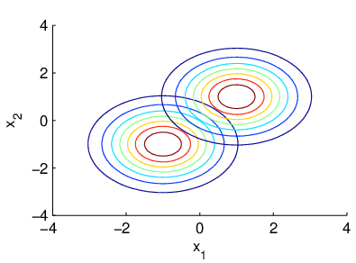


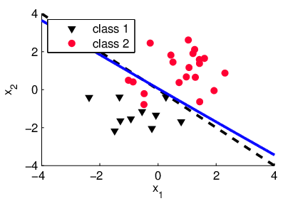
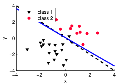
An example of the labeling problem is illustrated in Figure 1. Figure 1(1(a)) denotes the densities of the two classes. Figure 1(1(b)) denotes samples drawn from a mixture of the two original densities. Because the two clusters are highly overlapping, it may not be possible to properly label them by a clustering method.
In this paper we show that if one more dataset with a different class balance is available (Figure 1(1(c))), the labeling problem can be solved (Figures 1(1(d)) and 1(1(e))). More specifically, we show that a labeling for the samples can be obtained by estimating the sign of the difference between probability densities of two unlabeled datasets. A naive way is to first separately estimate two densities from two sets of samples and then take the sign of their difference to obtain a labeling. However, this naive procedure violates Vapnik’s principle[1]:
If you possess a restricted amount of information for solving some problem, try to solve the problem directly and never solve a more general problem as an intermediate step. It is possible that the available information is sufficient for a direct solution but is insufficient for solving a more general intermediate problem.
This principle was used in the development of support vector machines (SVMs): Rather than modeling two classes of samples, SVM directly learns a decision boundary that is sufficient for performing pattern recognition.
In the current context, estimating two densities is more general than labeling samples. Thus, the above naive scheme may be improved by estimating the density difference directly and then taking its sign to obtain the class labels. Recently, a method was introduced to directly estimate the density difference, called the least-squares density difference (LSDD) estimator [2]. Thus, the use of LSDD for labeling is expected to improve the performance.
However, the LSDD-based procedure is still indirect; directly estimating the sign of the density difference would be the most suitable approach to labeling. In this paper, we show that the sign of the density difference can be directly estimated by lower-bounding the -distance between probability densities. Based on this, we give a practical algorithm for labeling and illustrate its usefulness through experiments on various real-world datasets.
2 Problem Formulation and Fundamental Approaches
In this section, we formulate the problem of labeling, give our fundamental strategy, and consider two naive approaches.
2.1 Problem Formulation
Suppose that there are two probability distributions and on and , which are different only in class balances:
| (1) |
From these distributions, we are given two sets of unlabeled samples:
The goal of labeling is to obtain a labeling for the two sets of samples, and , that corresponds to the underlying class labels and . However, different from classification, we do not obtain correct class labels, but we obtain correct class separation up to label commutation.
2.2 Fundamental strategy
We wish to obtain a labeling for samples in and . Here we show that we can obtain the solution for the case where the class priors are equal. We may write the class-posterior distribution for the equal prior case as
where . A class label can then be assigned to a point by evaluating
We can write the criterion as
We do not have any labeled samples to calculate , but we can rewrite it in terms of marginal distributions. To see this, the above is multiplied with , which gives
Note that the sign may change since may be positive or negative. To write the third and fourth term as a joint distribution, we add and subtract , giving
Since and , we can express the above as
The exact class labels can not be recovered since the term can be positive or negative. Therefore, we assign the label to a point according to the following criterion:
| (2) |
Thus, now we need a good method to estimate .
2.3 Kernel Density Estimation
2.4 Direct Estimation of the Density Difference
KDE is a nice density estimator, but it is not necessarily suitable in density-difference estimation, because small estimation error incurred in each density estimate can cause a big error in the final density-difference estimate. More intuitively, good density estimators tend to be smooth and thus a density-difference estimator obtained from such smooth density estimators tends to be over-smoothed [5, 6].
The density difference can be estimated in a single shot using the least-squares density difference (LSDD) approach [2]. In this approach, we directly fit a model to the density difference under the square loss:
which can be efficiently obtained for a kernel density-difference model. A comprehensive review of LSDD is provided in Appendix 0.B. Finally, a labeling is obtained as
3 Direct Estimation of the Sign of the Density Difference
We expect that an improved solution can be obtained by LSDD over KDEs due to more direct nature of LSDD. However, LSDD is still indirect because the sign of density difference is inspected after the density difference is estimated. In this section, we show how to directly estimate the sign of the density difference.
3.1 Derivation of the Objective Function
By lower-bounding the -distance between probability densities, defined as
| (4) |
we can obtain the sign of the density difference. We begin by considering the following self-evident relation:
We can apply this relation at each point , to obtain
By applying the above inequality to Eq.(4) and maximizing with respect to , we can obtain the tightest lower bound as
| (5) | ||||
It is straightforward to verify that the above relation will be met with equality when
What makes the expression in the right-hand side of Eq.(5) especially useful is that the probability densities occur linearly in the integral. By replacing the integrals with sample averages and searching from a parametric family (denoted as ), we can write the above as
3.2 Optimization
Here we briefly discuss how to solve the problem in Eq. (3.1). A more detailed explanation is given in Appendix 0.A.
The function in Eq. (3.1) should satisfy the constraint . We can consider a clipped version of the function that always satisfies the constraint,
We use a linear-in-parameter model,
where are the basis functions. Using the above definitions, we can rewrite Eq.(3.1) as
| (8) |
where is a regularization term. Although the above is a non-convex problem, we can efficiently find a local optimal solution using the convex-concave procedure (CCCP) [7] (also known as difference of convex (d.c.) programming [8]). The CCCP procedure requires the objective function to be split into a convex and concave part,
The concave part is then upper-bounded as
where the bound is specified by and (details are given in Appendix 0.A). This bound is convex w.r.t. and if is fixed. Using this bound, the optimization problem can then be expressed as
The strategy to minimize is then to alternately minimize the right-hand side by minimizing w.r.t. (keeping and constant) and minimize w.r.t. and (keeping constant). Minimization w.r.t. minimizes the current upper bound and minimization w.r.t. and corresponds to tightening the bound at the current point.
Minimization w.r.t. and can be performed by
| (9) |
Minimization of the upper bound (assuming and is constant) can be performed by solving the following convex quadratic problem:
The above constrained problem can be solved with an off-the-shelf QP solver.
Our final optimization algorithm is summarized below:
- 1.
Initialize the starting value:
- 2.
In practice, Gaussian kernels centered at the sample points in and are chosen as the basis functions. All hyper-parameters are set by cross-validation.
4 Experiments
We first illustrate the operation of our method and characterize the failures of other methods on various toy examples. Then we use real-world benchmark data to show the superiority of our algorithm.
4.1 Numerical Illustration
Toy Problem 1:
We illustrate the problem and our method with a simple example. Suppose that the class-conditional densities for the two classes are given as
where denotes the normal density with mean and covariance w.r.t. . is a vector of ones and is a identity matrix. We generate sets of samples with class-priors and , respectively. The result is illustrated in Figure 1. As can be seen from this example, we are able to obtain a labeling of the classes that roughly corresponds to the true (unknown) labels of the data.
Toy Problem 2:
One way to obtain a labeling is to use clustering. The tacit assumption in clustering is that samples in the same cluster belong the same class. This assumption however is not always be true, for example, when the class conditional densities are multimodal. Here we consider a problem with the following class conditional densities:
The two distributions are plotted in Figure 2(a). We can try to obtain a class label by performing clustering on 11 1 If clustering is performed separately on and , we do not know which clusters in each dataset correspond to the clusters in the other dataset. We can also not perform clustering on one dataset and apply it to the other dataset, since most clustering methods do not give out of sample labeling. For these reasons, it makes most sense to perform clustering on the combined dataset.. The results for k-means and spectral clustering, given in Figures 2(d) and 2(e), show that these methods fail to reveal the true labeling. On the other hand, the proposed method still gives a reasonable result (Figure 2(f)).


4.2 Benchmark Datasets
We compare our method against several competing methods on benchmark datasets. For each experiment, we constructed the datasets and by drawing and samples from the positive and negative classes of the datasets according to a prior of and . The labeling was then performed using these two datasets. Since we can obtain a labeling, but cannot determine the original class labels, we cannot measure the performance using the misclassification rate directly. Assume that the label assigned for the sample is
The misclassification rate (MCR) assuming that the current labels are correct is
The misclassification rate assuming that the labels are the opposite is . We define the labeling error rate (LER) as
Note that this definition is somewhat more optimistic than using the misclassification rate. The smaller the dataset is, the lower the error would be for randomly assigning labels to samples: The expected LER for randomly assigning labels to samples (with equal probability) is
For , the expected labeling error rate is .
We compared the following methods:
- •
Direct Sign Density Difference (DSDD) Estimation (proposed): Directly estimate using the method described in Section 3. Hyperparameters are selected via cross validation.
- •
Least-Squares Density Difference (LSDD) Estimation: Estimate by estimating using the least squares fitting method [9]. Hyperparameters are selected via cross validation.
- •
Kernel Density Estimation (KDE): Estimate by estimating the densities and with kernel density estimation (KDE). Hyperparameters are selected using least-squares cross validation.
- •
K-Means (KM): Cluster the data into two clusters using the K-means algorithm.
- •
Spectral Clustering (SC): Cluster the data into two clusters using the spectral clustering algorithm [10]. The affinity matrix was constructed with nearest neighbors.
- •
Squared-loss Mutual Information based Clustering (SMIC) : Cluster the data according to the SMIC method [11]. SMIC was chosen since it provides model selection, avoiding the need for subjective parameter tuning.
We compare the performance of the methods by varying the class balance. Two class balances were selected: one with a large difference between the classes ( and ) and one with a small difference between the two priors ( and ). The average labeling error rate and standard deviation of the two experiments, with is given in Tables 1 and 2.
| Dataset | DSDD | LSDD | KDE | KM | SC | SMIC | ||||||
|---|---|---|---|---|---|---|---|---|---|---|---|---|
| australian | .142 | (.045) | .174 | (.110) | .211 | (.126) | .266 | (.147) | .381 | (.033) | .303 | (.103) |
| banana | .179 | (.097) | .170 | (.070) | .237 | (.147) | .431 | (.068) | .427 | (.141) | .424 | (.141) |
| diabetes | .246 | (.122) | .223 | (.079) | .226 | (.051) | .372 | (.080) | .380 | (.094) | .370 | (.131) |
| german | .268 | (.059) | .281 | (.127) | .211 | (.051) | .437 | (.114) | .448 | (.128) | .439 | (.052) |
| heart | .176 | (.051) | .174 | (.047) | .211 | (.074) | .261 | (.131) | .310 | (.032) | .327 | (.107) |
| image | .198 | (.078) | .206 | (.047) | .201 | (.049) | .385 | (.093) | .351 | (.119) | .384 | (.135) |
| ionosphere | .157 | (.059) | .184 | (.106) | .194 | (.123) | .329 | (.145) | .319 | (.113) | .311 | (.174) |
| saheart | .310 | (.093) | .205 | (.048) | .238 | (.113) | .422 | (.121) | .395 | (.113) | .384 | (.072) |
| thyroid | .102 | (.052) | .121 | (.116) | .207 | (.074) | .328 | (.113) | .326 | (.109) | .305 | (.074) |
| twonorm | .044 | (.085) | .051 | (.072) | .200 | (.028) | .036 | (.054) | .043 | (.069) | .048 | (.071) |
| Dataset | DSDD | LSDD | KDE | KM | SC | SMIC | ||||||
|---|---|---|---|---|---|---|---|---|---|---|---|---|
| australian | .244 | (.116) | .259 | (.088) | .355 | (.104) | .265 | (.080) | .376 | (.065) | .308 | (.107) |
| banana | .338 | (.094) | .339 | (.100) | .365 | (.067) | .433 | (.049) | .427 | (.069) | .424 | (.070) |
| diabetes | .340 | (.075) | .361 | (.124) | .345 | (.034) | .373 | (.063) | .380 | (.048) | .371 | (.114) |
| german | .375 | (.042) | .380 | (.093) | .354 | (.057) | .437 | (.024) | .445 | (.057) | .438 | (.041) |
| heart | .270 | (.133) | .247 | (.084) | .354 | (.052) | .264 | (.059) | .315 | (.081) | .327 | (.089) |
| image | .331 | (.078) | .350 | (.067) | .350 | (.039) | .384 | (.031) | .354 | (.049) | .382 | (.050) |
| ionosphere | .291 | (.099) | .356 | (.066) | .345 | (.048) | .330 | (.070) | .322 | (.058) | .314 | (.107) |
| saheart | .378 | (.093) | .353 | (.057) | .363 | (.066) | .419 | (.082) | .395 | (.022) | .385 | (.040) |
| thyroid | .227 | (.098) | .251 | (.087) | .302 | (.022) | .326 | (.061) | .329 | (.047) | .307 | (.076) |
| twonorm | .164 | (.188) | .153 | (.121) | .352 | (.096) | .036 | (.053) | .042 | (.122) | .049 | (.120) |
From the results we see that methods which follow the approach proposed in Section 2 of estimating the sign of the density difference (i.e., DSDD, LSDD, and KDE) generally work better than methods using the cluster structure of the data (i.e., KM, SC and SMIC). The thyroid dataset lends itself to interpretation of why these methods work better. The labels in the thyroid dataset correspond to healthy and diseased. The diseased label is caused by either a hyper-functioning or hypo-functioning thyroid. These two underlying causes cause within-class multimodality which may cause clustering-based methods to fail.
Among the methods which estimate the sign of the density difference, we see that DSDD generally performs better than LSDD and LSDD in turn performs better than KDE. This is as expected since KDE solves a more general problem than LSDD, and LSDD solves a more general problem than DSDD. This pattern is even more pronounced on the more difficult case where the class balances are close to each other (Table 2).
5 Conclusion
The problem of unsupervised labeling of two unbalanced datasets was considered. We first showed that this problem can be solved if two unlabeled datasets having different class balances are available. The solution can be obtained by estimating of the sign of the difference between probability densities. We introduced a method to directly estimate the sign of the density difference and avoid density estimation. The method was shown on various datasets to outperform competing methods that either estimate the density difference or use the cluster structure of the data.
Because the sign of density difference corresponds to the Bayes optimal classifier under equal class balance, it may be estimated by any classifier that separates and . Following this idea, we tested the support vector machine (SVM) for estimating the sign of density difference. However, this did not work well due to the high overlap of and —both the datasets are mixtures of two classes, only with different mixing ratios.
From this classification point of view, we can actually see that our objective function (8) corresponds to the robust SVM [12] that minimizes the ramp loss (a clipped hinge loss). Thanks to the robustness brought by the ramp loss, the overlapped datasets and can be separated more reliably, and thus we obtained good estimation of the sign of density difference.
Furthermore, this view conversely shows that the robust SVM is actually a suitable classification method because it directly estimates the Bayes optimal classifier, the sign of density difference. Labeling and classification are different problems, but one can actually give insight into the other. In the future work, we will further investigate the relation between labeling and classification.
References
- [1] Vapnik, V.: The Nature of Statistical Learning Theory. Statistics for Engineering and Information Science Series. Springer (2000)
- [2] Sugiyama, M., Kanamori, T., Suzuki, T., du Plessis, M.C., Liu, S., Takeuchi, I.: Density-difference estimation. In Bartlett, P., Pereira, F., Burges, C., Bottou, L., Weinberger, K., eds.: Advances in Neural Information Processing Systems 25. (2012) 692–700
- [3] Silverman, B.: Density estimation for statistics and data analysis. Chapman and Hall, London, UK (1986)
- [4] Härdle, W., Müller, M., Sperlich, S., Werwatz, A.: Nonparametric and semiparametric models. Springer (2004)
- [5] Hall, P., Wand, M.P.: On nonparametric discrimination using density differences. Biometrika 75(3) (1988) 541–547
- [6] Anderson, N.H., Hall, P., Titterington, D.: Two-sample test statistics for measuring discrepancies between two multivariate probability density functions using kernel-based density estimates. Journal of Multivariate Analysis 50(1) (1994) 41–54
- [7] Yuille, A.L., Rangarajan, A.: The concave-convex procedure (CCCP). In: Advances in Neural Information Processing Systems 14, MIT Press (2002)
- [8] Horst, R., Thoai, N.V.: DC programming: overview. Journal of Optimization Theory and Applications 103(1) (1999) 1–43
- [9] Sugiyama, M., Kanamori, T., Suzuki, T., du Plessis, M.C., Liu, S., Takeuchi, I.: Density-difference estimation. Neural Computation (2013) to appear.
- [10] Shi, J., Malik, J.: Normalized cuts and image segmentation. Pattern Analysis and Machine Intelligence, IEEE Transactions on 22(8) (2000) 888–905
- [11] Sugiyama, M., Yamada, M., Kimura, M., Hachiya, H.: On information-maximization clustering: Tuning parameter selection and analytic solution. In Getoor, L., Scheffer, T., eds.: Proceedings of 28th International Conference on Machine Learning (ICML2011), Bellevue, Washington, USA (Jun. 28–Jul. 2 2011) 65–72
- [12] Shawe-Taylor, J., Cristianini, N.: Kernel Methods for Pattern Analysis. Cambridge University Press, New York, NY, USA (2004)
Appendix 0.A Optimization
This section outlines the optimization of Eq. (8) using the convex concave procedure[7]. The non-convex function can be re-written as
The convex part of the objective function can then be expressed as
and the concave part as
The following self-evident relation can be used to bound the concave part
where
is known as the convex conjugate. The convex conjugate of the function is
This gives an upper bound on the concave function as
where and specify the bound.
0.A.1 Tightening the bound
The bound can be tightened around by minimizing w.r.t. and . To ensure that we have a non-trivial bound, we can explicitly write the conjugate as constraints,
The above optimization problem is separable in all unknowns, and the optimal value can be obtained by Eq. (9).
0.A.2 Minimizing the upper bound
The upper bound of the objective function with and is
By replacing each function with a slack variable , and the constraint
we obtain the objective function in Eq. (3.2)
Appendix 0.B Least-squares estimation of the density difference
In [9] it was proposed to directly estimate the density difference by fitting a model to the true density difference under a square loss:
The density difference was modeled by a linear-in-parameter model :
| (13) |
where denotes the number of basis functions, is a -dimensional basis function vector, is a -dimensional parameter vector, and ⊤ denotes the transpose. A Gaussian kernel model is used to model the density difference:
where are Gaussian kernel centers. For the model in Eq. (13), the optimal parameter is given by
where is the matrix and is the -dimensional vector defined as
For the Gaussian kernel model, the integral in can be computed analytically as
where is the dimensionality of .
Replacing the expectations in by empirical estimators and adding an -regularizer to the objective function, we arrive at the following optimization problem:
| (14) |
where () is the regularization parameter and is the -dimensional vector defined as
Taking the derivative of the objective function in Eq.(14) and equating it to zero, we can obtain the solution analytically as
where denotes the -dimensional identity matrix. Finally, the density difference estimator is