跳到论文正文
W Papers独立论文阅读器 arXiv:1305.0089 论文正文 计算阅读时间 · 0%
引用这篇论文根据当前论文元数据生成,正式投稿前建议核对。


License: arXiv.org perpetual non-exclusive license
arXiv:1305.0089v1 [math.NA] 01 May 2013

Approximation Properties of a Gradient Recovery Operator Using a Biorthogonal System

Bishnu P. Lamichhane11footnotemark: 1    Adam McNeilly ††thanks: School of Mathematical and Physical Sciences, University of Newcastle, Callaghan, NSW 2308, bishnu.lamichhane@newcastle.edu.au, adam.mcneilly@uon.edu.au
Abstract

A gradient recovery operator based on projecting the discrete gradient onto the standard finite element space is considered. We use an oblique projection, where the test and trial spaces are different, and the bases of these two spaces form a biorthogonal system. Biorthogonality allows efficient computation of the recovery operator. We analyse the approximation properties of the gradient recovery operator.

Key words. Gradient reconstruction, oblique projection, biorthogonal system
AMS subject classification. 65N30, 65N15, 65N50

1 Introduction

The gradient reconstruction is a popular technique to develop a reliable a posteriori error estimators for approximating the solution of partial differential equations using adaptive finite element methods [12, 13, 1, 9, 3, 2]. Recently we have presented a gradient reconstruction operator based on an oblique projection [5]. The oblique projection operator is constructed by using a biorthogonal system. In fact, for the linear finite element in simplicial meshes, this approach reproduces the so-called gradient reconstruction scheme by the weighted averaging [4, 9, 2]. We proved that the approximation property of the recovered gradient for any finite element space is similar to the one obtained by using the orthogonal projection with respect to L2L^{2}-norm [9, 3]. In this article, we aim at analysing the approximation property of the recovered gradient in one dimension using the oblique projection. This construction is quite useful in extending the weighted average gradient recovery of linear finite elements [9] to quadrilaterals and hexahedras.

Let Ω=(α,β)\Omega=(\alpha,\beta) with α,β∈ℝ\alpha,\beta\in\mathbb{R} and α<β\alpha<\beta. Let Δ={α=x0<x1<…<xn=β}\Delta=\left\{\alpha=x_{0}<x_{1}<...<x_{n}=\beta\right\} be a partition of the interval Ω\Omega. We define the interior of the grid, denoted i​n​t​(Δ)int\left(\Delta\right), as

i​n​t​(Δ)={xi∈Δ: 1≤i≤n−1}.int\left(\Delta\right)=\left\{x_{i}\in\Delta\,:\,1\leq i\leq n-1\right\}.

We also define the set of intervals in the partition Δ\Delta as {Ii}i=0n−1\left\{I_{i}\right\}_{i=0}^{n-1}, where Ii=[xi,xi+1)I_{i}=[x_{i},\,x_{i+1}). Two sets AnA_{n} and BnB_{n} of indices are also defined as An={i∈ℕ: 0≤i≤n}A_{n}=\left\{i\in\mathbb{N}\,:\,0\leq i\leq n\right\} and Bn=An∖{0,n}B_{n}=A_{n}\setminus\left\{0,\,n\right\}, respectively. A piecewise linear interpolant of a continuous function uu is written as Ih​u∈VhI_{h}u\in V_{h} with

Ih​u​(x)=∑i=0nu⁡(xi)​ϕi​(x),I_{h}u(x)=\sum_{i=0}^{n}u(x_{i})\phi_{i}(x),

where ϕi\phi_{i} is the standard hat function associated with the point xix_{i}, 0≤i≤n0\leq i\leq n. We define a discrete space,

Vh=span⁡{ϕ0,…,ϕn}⊂H1​(Ω).V_{h}=\mathrm{span}\left\{\phi_{0},\,...\,,\phi_{n}\right\}\subset H^{1}\left(\Omega\right).

The linear interpolant of u∈H1​(Ω)u\in H^{1}(\Omega) is the continuous function defined by Ih​u=∑i=0nu⁡(xi)​ϕiI_{h}u=\sum_{i=0}^{n}u(x_{i})\phi_{i}. However, if we compute the derivative of this interpolant Ih​uI_{h}u, the resulting function will not be continuous. To make the derivative continuous we project the derivative of the interpolant, ∂uh∂x=∑i=0nu⁡(xi)​∂ϕi∂x\frac{\partial u_{h}}{\partial x}=\sum_{i=0}^{n}u(x_{i})\,\frac{\partial\phi_{i}}{\partial x}, onto the discrete space VhV_{h}. There are two different types of projection. One is an orthogonal projection and the other is an oblique projection. The orthogonal projection operator, PhP_{h}, that projects ∂uh∂x\frac{\partial u_{h}}{\partial x} onto VhV_{h} is to find a gh=Ph​∂uh∂x∈Vhg_{h}=P_{h}\frac{\partial u_{h}}{\partial x}\in V_{h} that satisfies:

∫Ωgh​ϕj​𝑑x=∫Ω∂uh∂x​ϕj​𝑑x.\int_{\Omega}g_{h}\phi_{j}\,dx=\int_{\Omega}\frac{\partial u_{h}}{\partial x}\phi_{j}\,dx. (1.1)

Since gh∈Vhg_{h}\in V_{h}, we can represent it as an (n+1)\left(n+1\right)-dimensional vector:

g→=(g0⋮gn)​with​gh=∑i=0ngi​ϕi.\vec{g}=\left(\begin{array}[]{c}g_{0}\\ \vdots\\ g_{n}\end{array}\right)\,\mathrm{with}\;g_{h}=\sum_{i=0}^{n}g_{i}\phi_{i}.

Now the requirement given in equation (1.1) is equivalent to a linear system: M​g→=f→M\vec{g}=\vec{f}, where MM is a mass matrix, and

f→=(f0⋮fn)​with​fj=∫Ω∂uh∂x​ϕj​𝑑x.\vec{f}=\left(\begin{array}[]{c}f_{0}\\ \vdots\\ f_{n}\end{array}\right)\,\mathrm{with}\>f_{j}=\int_{\Omega}\frac{\partial u_{h}}{\partial x}\phi_{j}\,dx.

Here the mass matrix MM is tridiagonal. We can reduce computation time greatly if we have a diagonal mass matrix. This can be done if we use a suitable oblique projection instead of an orthogonal projection. We consider the projection

Qh:L2​(Ω)→Vh,Q_{h}:L^{2}(\Omega)\rightarrow V_{h},

which is defined as the problem of finding gh=Qh​d​ud​x∈Vhg_{h}=Q_{h}\frac{du}{dx}\in V_{h} such that

∫Ωgh​λh​𝑑x=∫Ωd​uhd​x​λh​𝑑x,λh∈Mh,\int_{\Omega}g_{h}\lambda_{h}\,dx=\int_{\Omega}\frac{du_{h}}{dx}\lambda_{h}\,dx,\qquad\lambda_{h}\in M_{h},

where MhM_{h} is another piecewise polynomial space, not orthogonal to VhV_{h}, with dim(Mh)=dim(Vh)\dim\left(M_{h}\right)=\dim\left(V_{h}\right), see [8]. In fact, the projection operator QhQ_{h} is well-defined due to the following stability condition. There is a constant β>0\beta>0 independent of the mesh-size hh such that [5, 6]

‖ϕh‖L2​(Ω)≤β​supμh∈Mh\{0}∫Ωμh​ϕh​𝑑x‖μh‖L2​(Ω),ϕh∈Vh.\displaystyle\|\phi_{h}\|_{L^{2}(\Omega)}\leq\beta\sup_{\mu_{h}\in M_{h}\backslash\{0\}}\frac{\int_{\Omega}\mu_{h}\phi_{h}\,dx}{\|\mu_{h}\|_{L^{2}(\Omega)}},\quad\phi_{h}\in V_{h}.

In order to achieve that the mass matrix MM is diagonal we need to define a new set of basis functions for MhM_{h}, {λ0,…,λn}\left\{\lambda_{0},\,...\,,\lambda_{n}\right\}, that are biorthogonal to the standard hat basis function we used previously. This biorthogonality relation is defined as:

∫Ωλi​ϕj​𝑑x=cj​δi​j,cj≠0, 1≤i,j≤n,\int_{\Omega}\lambda_{i}\phi_{j}dx=c_{j}\delta_{ij},\,c_{j}\not=0,\,1\leq i,\,j\leq n, (1.2)

where δi​j\delta_{ij} is the Kronecker delta function:

δi​j={1,if​i=j0,otherwise,\delta_{ij}=\begin{cases}1,&\mathrm{if}\,i=j\\ 0,&\mathrm{otherwise}\end{cases},

and cjc_{j} is a positive scaling factor. The basis functions for MhM_{h} are simply given by

λ0​(x)\displaystyle\lambda_{0}(x) ={2​(x−x1)+(x−x0)x0−x1,x0≤x≤x10,otherwise\displaystyle=\begin{cases}\frac{2(x-x_{1})+(x-x_{0})}{x_{0}-x_{1}},&x_{0}\leq x\leq x_{1}\\ 0\,,&\mathrm{otherwise}\end{cases}
λn​(x)\displaystyle\lambda_{n}(x) ={2​(x−xn−1)+(x−xn)xn−xn−1,xn−1≤x≤xn0,otherwise,\displaystyle=\begin{cases}\frac{2(x-x_{n-1})+(x-x_{n})}{x_{n}-x_{n-1}},&x_{n-1}\leq x\leq x_{n}\\ 0\,,&\mathrm{otherwise}\end{cases},

and for 1≤i≤n−11\leq i\leq n-1

λi​(x)\displaystyle\lambda_{i}(x) ={2​(x−xi−1)+(x−xi)xi−xi−1,xi−1≤x≤xi2​(x−xi+1)+(x−xi)xi−xi+1,xi≤x≤xi+10,otherwise.\displaystyle=\begin{cases}\frac{2(x-x_{i-1})+(x-x_{i})}{x_{i}-x_{i-1}},&x_{i-1}\leq x\leq x_{i}\\ \frac{2(x-x_{i+1})+(x-x_{i})}{x_{i}-x_{i+1}},&x_{i}\leq x\leq x_{i+1}\\ 0\,,&\mathrm{otherwise}\end{cases}.
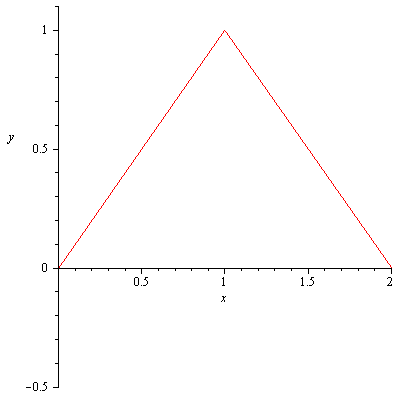
Refer to caption
Refer to caption
Figure 1: The hat basis function (left) and biorthogonal basis function (right) with stepsize h=1h=1.

By using an oblique projection QhQ_{h} the mass matrix will be diagonal. We let the diagonal mass matrix be D, so that our system is D​g→=f→D\vec{g}=\vec{f}. The values gig_{i} are our estimates of the gradient of uu at the point xix_{i}. So, we estimate the gradient by finding g→=D−1​f→\vec{g}=D^{-1}\vec{f}, where

gi=∫x0xnd​uhd​x​λi​𝑑x∫x0xnϕi​λi​𝑑x.g_{i}=\frac{\int_{x_{0}}^{x_{n}}\frac{du_{h}}{dx}\lambda_{i}dx}{\int_{x_{0}}^{x_{n}}\phi_{i}\lambda_{i}dx}.

We want to calculate the error in this approximation, and find out when gig_{i} approximates u′​(xi)u^{\prime}(x_{i}) exactly for each xi∈Δx_{i}\in\Delta. As in [10, 11] we want to see if gig_{i} approximates u′​(xi)u^{\prime}(x_{i}) exactly when uu is a quadratic polynomial.

2 Superconvergence

Theorem 1

Let u∈C0​(Ω)u\in C^{0}(\Omega). Then we have

gi=u⁡(xi+1)−u⁡(xi−1)xi+1−xi−1,i∈Bn,g_{i}=\frac{u(x_{i+1})-u(x_{i-1})}{x_{i+1}-x_{i-1}},\quad i\in B_{n},

and

g0=u⁡(x1)−u⁡(x0)x1−x0,gn=u⁡(xn)−u⁡(xn−1)xn−xn−1.g_{0}=\frac{u(x_{1})-u(x_{0})}{x_{1}-x_{0}},\quad g_{n}=\frac{u(x_{n})-u(x_{n-1})}{x_{n}-x_{n-1}}.

Proof:  We note that

λi​(x)={2​(x−xi−1)+(x−xi)xi−xi−1,xi−1≤x≤xi2​(x−xi+1)+(x−xi)xi−xi+1xi≤x≤xi+10,otherwise,for​all​i∈Bn.\lambda_{i}(x)=\begin{cases}\frac{2(x-x_{i-1})+(x-x_{i})}{x_{i}-x_{i-1}},&x_{i-1}\leq x\leq x_{i}\\ \frac{2(x-x_{i+1})+(x-x_{i})}{x_{i}-x_{i+1}}&x_{i}\leq x\leq x_{i+1}\\ 0\,,&\mathrm{otherwise}\end{cases},\>\mathrm{for\,all}\>i\in B_{n}.

Now, we calculate gig_{i} for i∈Bni\in B_{n}:

gi=∫x0xnd​uhd​x​λi​𝑑x∫x0xnϕi​λi​𝑑x,g_{i}=\frac{\int_{x_{0}}^{x_{n}}\frac{du_{h}}{dx}\lambda_{i}\,dx}{\int_{x_{0}}^{x_{n}}\phi_{i}\lambda_{i}\,dx},

where

∫x0xnϕi​λi​𝑑x\displaystyle\int_{x_{0}}^{x_{n}}\phi_{i}\lambda_{i}dx =∫xi−1xi(x−xi−1xi−xi−1)​(2​(x−xi−1)+(x−xi)xi−xi−1)​𝑑x\displaystyle=\int_{x_{i-1}}^{x_{i}}\left(\frac{x-x_{i-1}}{x_{i}-x_{i-1}}\right)\left(\frac{2\left(x-x_{i-1}\right)+\left(x-x_{i}\right)}{x_{i}-x_{i-1}}\right)dx
+∫xixi+1(x−xi+1xi−xi+1)(2​(x−xi+1)+(x−xi)xi−xi+1)dx\displaystyle+\int_{x_{i}}^{x_{i+1}}\left(\frac{x-x_{i+1}}{x_{i}-x_{i+1}}\right)\left(\frac{2\left(x-x_{i+1}\right)+\left(x-x_{i}\right)}{x_{i}-x_{i+1}}\right)dx
=−12​(xi−1−xi+1),\displaystyle=-\frac{1}{2}\left(x_{i-1}-x_{i+1}\right),

and

∫x0xnd​uhd​x​λi​𝑑x\displaystyle\qquad\int_{x_{0}}^{x_{n}}\frac{du_{h}}{dx}\lambda_{i}\,dx =∑j=0nu⁡(xj)​∫x0xnd​ϕjd​x​λi​𝑑x\displaystyle=\sum_{j=0}^{n}u(x_{j})\int_{x_{0}}^{x_{n}}\frac{d\phi_{j}}{dx}\lambda_{i}\,dx
=u⁡(xi−1)​∫xi−1xid​ϕi−1d​x​λi​dx+u⁡(xi)​(∫xi−1xid​ϕid​x​λi​dx+∫xixi+1d​ϕid​x​λi​dx)\displaystyle=u(x_{i-1})\int_{x_{i-1}}^{x_{i}}\frac{d\phi_{i-1}}{dx}\lambda_{i}\,dx+u(x_{i})\left(\int_{x_{i-1}}^{x_{i}}\frac{d\phi_{i}}{dx}\lambda_{i}\,dx+\int_{x_{i}}^{x_{i+1}}\frac{d\phi_{i}}{dx}\lambda_{i}\,dx\right)
+u(xi+1)∫xixi+1d​ϕi+1d​xλidx\displaystyle+u(x_{i+1})\int_{x_{i}}^{x_{i+1}}\frac{d\phi_{i+1}}{dx}\lambda_{i}\,dx
(since​ϕj​and​λi​overlap​only​when​j∈{i−1,i,i+1})\displaystyle\mathrm{(since}\>\phi_{j}\>\mathrm{and}\>\lambda_{i}\>\mathrm{overlap\,only\,when}\,j\in\left\{i-1,\,i,\,i+1\right\}\mathrm{)}
Therefore,gi\displaystyle\mathrm{Therefore,\quad}g_{i} =u⁡(xi+1)−u⁡(xi−1)xi+1−xi−1.\displaystyle=\frac{u(x_{i+1})-u(x_{i-1})}{x_{i+1}-x_{i-1}}.

Now we look at the end-points. We note that

g0=∫x0xnd​uhd​x​λ0​𝑑x∫x0xnϕ0​λ0​𝑑x,andgn=∫x0xnd​uhd​x​λn​𝑑x∫x0xnϕn​λn​𝑑x.g_{0}=\frac{\int_{x_{0}}^{x_{n}}\frac{du_{h}}{dx}\lambda_{0}\,dx}{\int_{x_{0}}^{x_{n}}\phi_{0}\lambda_{0}\,dx},\quad\text{and}\quad g_{n}=\frac{\int_{x_{0}}^{x_{n}}\frac{du_{h}}{dx}\lambda_{n}\,dx}{\int_{x_{0}}^{x_{n}}\phi_{n}\lambda_{n}\,dx}.

Computing as before we get

g0=u⁡(x1)−u⁡(x0)x1−x0,gn=u⁡(xn)−u⁡(xn−1)xn−xn−1.g_{0}=\frac{u(x_{1})-u(x_{0})}{x_{1}-x_{0}},\quad g_{n}=\frac{u(x_{n})-u(x_{n-1})}{x_{n}-x_{n-1}}.
 

We have the following super-convergence in L2L^{2}-norm. This is proved as in [7, 9].

Theorem 2

Let hi=xi+1−xih_{i}=x_{i+1}-x_{i} for 0≤i≤n−10\leq i\leq n-1, h=max0≤i≤n−1⁡hih=\max_{0\leq i\leq n-1}h_{i}, and Ω0=(x1,xn−1)\Omega_{0}=(x_{1},x_{n-1}). If the point distribution satisfies |hi+1−hi|=O⁡(h2)|h_{i+1}-h_{i}|=O(h^{2}) for 0≤i≤n−10\leq i\leq n-1. Then we have the estimate

‖d​ud​x−Qh​d​uhd​x‖L2​(Ω0)≤h2​‖u‖W3,∞​(Ω0),u∈W3​∞​(Ω).\left\|\frac{du}{dx}-Q_{h}\frac{du_{h}}{dx}\right\|_{L^{2}(\Omega_{0})}\leq h^{2}\|u\|_{W^{3,\infty}(\Omega_{0})},\quad u\in W^{3\infty}(\Omega).

For the tensor product meshes in two or three dimensions satisfying the above mesh condition this theorem has an easy extension.

2.1 Application to quadratic functions

Corollary 3

Let u∈P2​(ℝ)u\in P_{2}\left(\mathbb{R}\right). Then gig_{i} reproduces u′​(x~i)u^{\prime}\left(\tilde{x}_{i}\right) exactly for all xi∈Δx_{i}\in\Delta, where:

x~i={x0+x12,i=0xi−1+xi+12,1≤i≤n−1xn−1+xn2,i=n,andgi=∫x0xnd​uhd​x​λi​𝑑x∫x0xnϕi​λi​𝑑x.\displaystyle\tilde{x}_{i}=\begin{cases}\frac{x_{0}+x_{1}}{2},&i=0\\ \frac{x_{i-1}+x_{i+1}}{2},&1\leq i\leq n-1\\ \frac{x_{n-1}+x_{n}}{2},&i=n\end{cases},\quad\text{and}\quad g_{i}=\frac{\int_{x_{0}}^{x_{n}}\frac{du_{h}}{dx}\,\lambda_{i}\,dx}{\int_{x_{0}}^{x_{n}}\phi_{i}\,\lambda_{i}\,dx}.
Refer to caption
Figure 2: A non-uniform grid with 8 nodes (vertical lines). The points x~i\tilde{x}_{i} (dots) are also shown.

Proof:  We use the result of the previous theorem to get

gi\displaystyle g_{i} =(a​xi−12+b​xi−1−a​xi+12−b​xi+1)(xi−1−xi+1)\displaystyle=\frac{\left(ax_{i-1}^{2}+bx_{i-1}-ax_{i+1}^{2}-bx_{i+1}\right)}{\left(x_{i-1}-x_{i+1}\right)}
=a⁡(xi−12−xi+12)+b⁡(xi−1−xi+1)xi−1−xi+1\displaystyle=\frac{a\left(x_{i-1}^{2}-x_{i+1}^{2}\right)+b\left(x_{i-1}-x_{i+1}\right)}{x_{i-1}-x_{i+1}}
=a⁡(xi−1−xi+1)​(xi−1+xi+1)+b⁡(xi−1−xi+1)xi−1−xi+1\displaystyle=\frac{a\left(x_{i-1}-x_{i+1}\right)\left(x_{i-1}+x_{i+1}\right)+b\left(x_{i-1}-x_{i+1}\right)}{x_{i-1}-x_{i+1}}
=a⁡(xi−1+xi+1)+b.\displaystyle=a\left(x_{i-1}+x_{i+1}\right)+b.

On the other hand,

u′​(x~i)\displaystyle u^{\prime}\left(\tilde{x}_{i}\right) =2​a​(xi−1+xi+12)+b\displaystyle=2a\left(\frac{x_{i-1}+x_{i+1}}{2}\right)+b
=a⁡(xi−1+xi+1)+b\displaystyle=a\left(x_{i-1}+x_{i+1}\right)+b
=gi.\displaystyle=g_{i}.

So, gig_{i} reproduces u′​(x~i)u^{\prime}\left(\tilde{x}_{i}\right) exactly for i∈Bni\in B_{n}. Now for i=0i=0 and i=ni=n, we have

g0\displaystyle g_{0} =12​(a​x12+b​x1−a​x02−b​x0)12​(x1−x0)=a⁡(x12−x02)+b⁡(x1−x0)x1−x0\displaystyle=\frac{\frac{1}{2}\left(ax_{1}^{2}+bx_{1}-ax_{0}^{2}-bx_{0}\right)}{\frac{1}{2}\left(x_{1}-x_{0}\right)}=\frac{a\left(x_{1}^{2}-x_{0}^{2}\right)+b\left(x_{1}-x_{0}\right)}{x_{1}-x_{0}}
=a⁡(x1−x0)​(x1+x0)+b⁡(x1−x0)x1−x0=a⁡(x1+x0)+b,\displaystyle=\frac{a\left(x_{1}-x_{0}\right)\left(x_{1}+x_{0}\right)+b\left(x_{1}-x_{0}\right)}{x_{1}-x_{0}}=a\left(x_{1}+x_{0}\right)+b,
andgn\displaystyle\quad\text{and}\quad g_{n} =12​(a​xn−12+b​xn−1−a​xn2−b​xn)12​(xn−1−xn)=a⁡(xn−12−xn2)+b⁡(xn−1−xn)xn−1−xn\displaystyle=\frac{\frac{1}{2}\left(ax_{n-1}^{2}+bx_{n-1}-ax_{n}^{2}-bx_{n}\right)}{\frac{1}{2}\left(x_{n-1}-x_{n}\right)}=\frac{a\left(x_{n-1}^{2}-x_{n}^{2}\right)+b\left(x_{n-1}-x_{n}\right)}{x_{n-1}-x_{n}}
=a⁡(xn−1−xn)​(xn−1+xn)+b⁡(xn−1−xn)xn−1−xn=a⁡(xn−1+xn)+b.\displaystyle=\frac{a\left(x_{n-1}-x_{n}\right)\left(x_{n-1}+x_{n}\right)+b\left(x_{n-1}-x_{n}\right)}{x_{n-1}-x_{n}}=a\left(x_{n-1}+x_{n}\right)+b.

Since

u′​(x~0)=a⁡(x0+x1)+b,andu′​(x~n)=a⁡(xn−1+xn)+b,u^{\prime}\left(\tilde{x}_{0}\right)=a\left(x_{0}+x_{1}\right)+b,\quad\text{and}\quad u^{\prime}\left(\tilde{x}_{n}\right)=a\left(x_{n-1}+x_{n}\right)+b,

we have g0g_{0} and gng_{n} reproduce u′​(x~0)u^{\prime}\left(\tilde{x}_{0}\right) and u′​(x~n)u^{\prime}\left(\tilde{x}_{n}\right), respectively, exactly.  

Remark 4 (Uniform Grid)

Let Δ={α=x0<x1<…<xn=β}\Delta=\left\{\alpha=x_{0}<x_{1}<...<x_{n}=\beta\right\} be a uniform grid on the interval Ω\Omega so that xi−xi−1=h,∀i∈An∖{0}x_{i}-x_{i-1}=h,\;\forall\,i\in A_{n}\setminus\left\{0\right\}, where hh is some constant, called the stepsize. We note that if our grid is uniform, then xi=x~i​∀xi∈i​n​t​(Δ)x_{i}=\tilde{x}_{i}\;\forall x_{i}\in int\left(\Delta\right). So, our gradient recovery operator will reproduce the exact gradient of any quadratic function on the interior of a uniform grid. We cannot recover the gradients at the endpoints exactly, however, since x0≠x~0x_{0}\not=\tilde{x}_{0} and xn≠x~nx_{n}\not=\tilde{x}_{n}.

Corollary 5

Let u∈P2​(ℝ)u\in P_{2}(\mathbb{R}) with u⁡(x)=a​x2+b​x+cu(x)=ax^{2}+bx+c, and let the grid be uniform with stepsize hh and x0=0x_{0}=0. Then |gi−u′​(xi)|=a​h\left|g_{i}-u^{\prime}(x_{i})\right|=ah for i=0,ni=0,\,n (i.e. for the endpoints of the grid).

Proof:  We will start with the case where i=0i=0 (i.e. the left endpoint). We know from Theorem 3 that g0=a⁡(x1−x0)+bg_{0}=a\left(x_{1}-x_{0}\right)+b. Since our grid is uniform with stepsize hh, this simplifies to g0=a​h+bg_{0}=ah+b. u′​(x0)=2​a​x0+b=bu^{\prime}\left(x_{0}\right)=2ax_{0}+b=b, since x0=0x_{0}=0. Therefore

|g0−u′​(x0)|\displaystyle\left|g_{0}-u^{\prime}\left(x_{0}\right)\right| =|(a​h+b)−b|\displaystyle=\left|\left(ah+b\right)-b\right|
=a​h.\displaystyle=ah.

The case for i=ni=n (i.e. the right endpoint) is proven similarly.  

For a non-uniform grid, we cannot simplify our approximations using the stepsize hh, since the spacing between each adjacent node is not always equal. We did not make any assumption about the uniformity of the grid in Theorem 3. Thus |gi−u′​(xi)||g_{i}-u^{\prime}(x_{i})|, i∈Ani\in A_{n}, is not zero for a non-uniform grid This is estimated in the following corollary.

Corollary 6

Let u⁡(x)=a​x2+b​x+cu\left(x\right)=ax^{2}+bx+c. Then,

|gi−u′​(xi)|\displaystyle\left|g_{i}-u^{\prime}\left(x_{i}\right)\right| =a⁡(xi−1+xi+1−2​xi)​∀xi∈i​n​t​(Δ),\displaystyle=a\left(x_{i-1}+x_{i+1}-2x_{i}\right)\>\forall x_{i}\in int\left(\Delta\right),
|g0−u′​(x0)|\displaystyle\left|g_{0}-u^{\prime}\left(x_{0}\right)\right| =a⁡(x1−x0),and\displaystyle=a\left(x_{1}-x_{0}\right),\,\mathrm{and}
|gn−u′​(xn)|\displaystyle\left|g_{n}-u^{\prime}\left(x_{n}\right)\right| =a⁡(xn−1−xn).\displaystyle=a\left(x_{n-1}-x_{n}\right).
Remark 7

For i∈Bni\in B_{n} let hi=xi+1−xih_{i}=x_{i+1}-x_{i}. Then we have

|gi−u′​(xi)|=a⁡(xi−1+xi+1−2​xi)=a⁡(hi+1−hi).\left|g_{i}-u^{\prime}\left(x_{i}\right)\right|=a\left(x_{i-1}+x_{i+1}-2x_{i}\right)=a(h_{i+1}-h_{i}).

We still get superapproximation of the gradient recovery when hi+1−hi=O⁡(h2)h_{i+1}-h_{i}=O(h^{2}) when i∈Bni\in B_{n}.

2.2 Application to cubic functions

Corollary 8

Let u∈P3​(ℝ)u\in P_{3}(\mathbb{R}) with u⁡(x)=a​x3+b​x2+c​x+du(x)=ax^{3}+bx^{2}+cx+d. Then,

|gi−u′​(x~i)|=a4​(xi−1−xi+1)2\left|g_{i}-u^{\prime}\left(\tilde{x}_{i}\right)\right|=\frac{a}{4}\left(x_{i-1}-x_{i+1}\right)^{2}

for all i∈Bni\in B_{n}, and

|g0−u′​(x~0)|\displaystyle\left|g_{0}-u^{\prime}\left(\tilde{x}_{0}\right)\right| =a4​(x0−x1)2\displaystyle=\frac{a}{4}\left(x_{0}-x_{1}\right)^{2}
|gn−u′​(x~n)|\displaystyle\left|g_{n}-u^{\prime}\left(\tilde{x}_{n}\right)\right| =a4​(xn−1−xn)2\displaystyle=\frac{a}{4}\left(x_{n-1}-x_{n}\right)^{2}

where x~i\tilde{x}_{i} is defined as in Theorem 3. Similarly, for all i∈Bni\in B_{n} we have

|gi−u′​(xi)|=a⁡(xi−12+xi−1​xi+1+xi+12−3​xi2)+b⁡(xi−1+xi+1−2​xi),\left|g_{i}-u^{\prime}(x_{i})\right|=a\left(x_{i-1}^{2}+x_{i-1}x_{i+1}+x_{i+1}^{2}-3x_{i}^{2}\right)+b\left(x_{i-1}+x_{i+1}-2x_{i}\right),

and

|g0−u′​(x0)|\displaystyle\left|g_{0}-u^{\prime}(x_{0})\right| =\displaystyle= a⁡(x12+x0​x1−2​x02)+b⁡(x1−x0),\displaystyle a\left(x_{1}^{2}+x_{0}x_{1}-2x_{0}^{2}\right)+b\left(x_{1}-x_{0}\right),
|gn−u′​(xn)|\displaystyle\left|g_{n}-u^{\prime}(x_{n})\right| =\displaystyle= a⁡(xn−12+xn−1​xn−2​xn2)+b⁡(xn−1−xn).\displaystyle a\left(x_{n-1}^{2}+x_{n-1}x_{n}-2x_{n}^{2}\right)+b\left(x_{n-1}-x_{n}\right).

Proof:  The proof of this theorem is similar to Theorem 3.  

3 Conclusion

We have presented an analysis of approximation property of the reconstructed gradient using an oblique projection. The reconstruction of the gradient is numerically efficient due to the use of a biorthogonal system. It is useful to investigate the extension to higher order finite elements.

References

  • [1] M. Ainsworth and J. T. Oden. A Posteriori Error Estimation in Finite Element Analysis. Wiley–Interscience, New York, 2000.
  • [2] J. Chen and D. Wang. Three-dimensional finite element superconvergent gradient recovery on par6 patterns. Numerical Marthematics: Theory, Methods and Applications, 3:178–194, 2010.
  • [3] L. Chen. Superconvergence of tetrahedral linear finite elements. International Journal of Numerical Analysis and Modeling,, 3:273–282, 2006.
  • [4] J. Goodsell. Pointwise superconvergence of the gradient for the linear tetrahedral element. Numerical Methods for Partial Differential Equations, 10:651–666, 1994.
  • [5] B.P. Lamichhane. A gradient recovery operator based on an oblique projection. Electronic Transactions on Numerical Analysis, 37:166–172, 2010.
  • [6] B.P. Lamichhane. A stabilized mixed finite element method for the biharmonic equation based on biorthogonal systems. Journal of Computational and Applied Mathematics, 235:5188–5197, 2011.
  • [7] B. Li and Z. Zhang. Analysis of a class of superconvergence patch recovery techniques for linear and bilinear finite elements. Numerical Methods for Partial Differential Equations, 15:151–167, 1999.
  • [8] B.I. Wohlmuth. Discretization Methods and Iterative Solvers Based on Domain Decomposition, volume 17 of LNCS. Springer Heidelberg, 2001.
  • [9] J. Xu and Z. Zhang. Analysis of recovery type a posteriori error estimators for mildly structured grids. Mathematics of Computation, 73:1139–1152, 2004.
  • [10] Z. Zhang. Ultraconvergence of the patch recovery technique. Mathematics of Computation, 65:1431 – 1437, 1996.
  • [11] Z. Zhang. Ultraconvergence of the patch recovery technique ii. Mathematics of Computation, 69:141 – 158, 2000.
  • [12] O.C. Zienkiewicz and J.Z. Zhu. The superconvergent patch recovery and a posteriori error estimates. part 1: The recovery technique. International Journal for Numerical Methods in Engineering, 33:1331–1364, 1992.
  • [13] O.C. Zienkiewicz and J.Z. Zhu. The superconvergent patch recovery and a posteriori error estimates. part 2: Error estimates and adaptivity. International Journal for Numerical Methods in Engineering, 33:1365–1382, 1992.