Quantum-Limited Mirror-Motion Estimation
Abstract
We experimentally demonstrate optomechanical motion and force measurements near the quantum precision limits set by the quantum Cramér-Rao bounds (QCRBs). Optical beams in coherent and phase-squeezed states are used to measure the motion of a mirror under an external stochastic force. Utilizing optical phase tracking and quantum smoothing techniques, we achieve position, momentum, and force estimation accuracies close to the QCRBs with the coherent state, while estimation using squeezed states shows clear quantum enhancements beyond the coherent-state bounds.
The advance of science and technology demands increasingly precise measurements of physical quantities. The probabilistic nature of quantum mechanics represents a fundamental roadblock. Over the last few decades, the issue of quantum limits to precision measurements has been a key driver in the development of quantum measurement theory [1, *wiseman_milburn, 3]. With the recent technological advances in quantum optical, electrical, atomic, and mechanical systems, quantum limits are now becoming relevant to many metrological applications, such as gravitational-wave detection [4], force sensing [5, *aspelmeyer], magnetometry [7], clocks [8], and biological measurements [9].
It is now recognized that quantum detection and estimation theory [10] provides the appropriate framework for the definition and proof of quantum measurement limits. For parameter estimation and the mean-square error (MSE) criterion, a widely studied quantum limit is the quantum Cramér-Rao bound (QCRB) [10, 11]. For gravitational-wave astronomy and many other sensing applications, the estimation of time-varying parameters, commonly called waveforms in the engineering literature, is more relevant. QCRBs for waveform estimation were recently derived in Refs. [12, *tsang_open], although there has not yet been any comparison of the waveform QCRBs with experimental results to demonstrate their relevance to current technology.
Quantum estimation of an optical phase waveform was recently demonstrated experimentally [14, 15] using an optical phase tracking method that measures the phase via homodyne detection with feedback control [16, *berry2002, *berry2006, *armen], followed by smoothing of the data [20, *tsl2009, 22, *smooth_pra1, *smooth_pra2]. These experiments demonstrate improvements over heterodyne measurements, causal filtering [14], and coherent-state optical beams when squeezed light is used [15], but no comparison with the QCRBs was made to test the optimality of the experimental techniques.
In this Letter, we report an experiment that applies the tracking and smoothing techniques to optomechanical motion sensing. We use optical probe beams in coherent and phase-squeezed states to measure the motion of a mirror under an external stochastic force and then compare the smoothing errors with the waveform QCRBs. This is the first time to our knowledge that experimental results have been compared with the waveform QCRBs. Through the comparison, we are able to demonstrate the near-optimality of our measurement method in the case of coherent states. The squeezed-state results are further away from the QCRBs but still show clear enhancements over the coherent-state bounds. Despite our focus here on a classical mechanical system, our methods can also be applied to purely quantum systems [20, *tsl2009, *smooth, *smooth_pra1, *smooth_pra2, 12, *tsang_open], making our methods potentially useful for a wide range of quantum sensing applications [3, 4, 5, *aspelmeyer, 7, 8, 9].
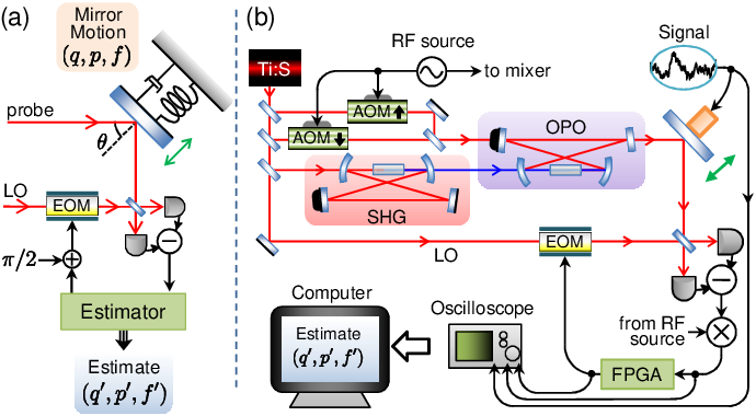
Figure 1(a) shows a schematic of our experiment, where the mirror motion is approximated as a mass-spring-damper system. The mirror, driven by a stochastic force, is illuminated by a probe beam in a coherent state or a phase-squeezed state. The motion of the mirror shifts the phase of the probe beam. We measure this phase shift adaptively by homodyne detection (optical phase tracking) [16, *berry2002, *berry2006, *armen, 14, 15], and estimate the mirror motion from the optical phase measurements [20, *tsl2009, *smooth, *smooth_pra1, *smooth_pra2].
Optical phase tracking allows us to linearize the measurement results as
| (1) |
where is the optical phase shift and is a noise term depending on the optical beam statistics [14, 15, 25]. The phase shift of the probe beam is caused by the mirror position shift as
| (2) |
where is the wave-vector component parallel to the mirror motion and is the reflecting angle as shown in Fig. 1 (a), fixed at . We estimate the mirror position , momentum , and external force from the measurement results . , , , and are assumed to be zero-mean stationary processes.
Under the linear approximation, the optimal estimate of the mirror position is a weighted sum of the measurement results given by , where is a linear filter and prime indicates an estimate. Estimates of momentum and external force are similarly defined. The integration limits are approximated as because we use data long before and after to obtain the estimates at the intermediate time via smoothing [20, *tsl2009, *smooth, *smooth_pra1, *smooth_pra2]. The optimal position filter is obtained by minimizing the MSE , which is averaged over the probability measures for and ( and are similarly defined). The optimal filters and the minimum MSEs are calculated by moving to the frequency domain [25]. The minimum MSEs () are given by [20, *tsl2009, *smooth, *smooth_pra1, *smooth_pra2, 26, 25]
| (3) |
where () is a spectral density defined as , is a transfer function that relates the optical phase shift to the target variables () by , with the tilde indicating a Fourier transform.
We now consider the QCRBs on the MSEs. The waveform QCRBs are derived from the quantum properties of the probe beams and prior statistics of the target system (mirror motion) and do not depend on the measurement and post-processing method. The QCRBs for our situation are [12, 13]
| (4) |
where is the spectral density of the probe-beam photon flux. Comparing Eq. (3) with Eq. (4), we find that is required for to match the QCRBs. This means that, to attain the QCRBs, (i) the probe beam should be in a minimum-uncertainty state with respect to the phase and the photon flux, and (ii) the measurement noise should consist of intrinsic phase noise only.
Our experiment uses broadband phase-squeezed states, including coherent states as the small-squeezing limit. The noise term in the normalized homodyne outputs can be written in a quadratic approximation [15, 25] as
| (5) | ||||
| (6) |
where is the squeezing (anti-squeezing) parameter , is the coherent amplitude of the probe beam, is the steady-state MSE of the optical phase estimate in the real-time feedback loop (). is called the effective squeezing factor [15], which takes into account the anti-squeezed amplitude quadrature as well as the squeezed phase quadrature. The noise spectral density and the photon-flux spectal density are [25]
| (7) |
Here we assume that the bandwidth of squeezing is broad compared to the bandwidth of system parameters, but not too large so that the photon-flux fluctuations do not diverge (see Supplemental Material [25]).
The necessary condition to reach the QCRBs is now given by . For coherent states ( and ), this condition is always satisfied, so QCRB-limited estimation is possible within the quadratic approximation. On the other hand, the squeezed-state QCRB is attainable only if (i) the squeezed state is pure () and (ii) the optical phase tracking works well enough such that . Thus, in a real experimental situation, the squeezed-state QCRB is more difficult to reach than the coherent-state QCRB. We emphasize however that our estimation results are still comparable to the squeeze-state QCRBs and better than the coherent-state bounds.
Figure 1(b) shows our experimental setup. A continuous-wave Titanium Sapphire laser is used as a light source at 860 nm. Phase-squeezed states are generated by an optical parametric oscillator (OPO) [15, 27]. The OPO is driven below threshold by a 430 nm pump beam. Optical sidebands at 5 MHz are used as a carrier beam generated by acousto-optic modulators [14, 15]. To avoid experimental complexities, the pump power is fixed at 80 mW, producing squeezing and anti-squeezing levels of dB and 6.000.15 dB. The effective squeezing factor, , varies from dB to dB depending on the probe amplitude. To make a coherent state, we simply block the pump beam.
A mirror (12.7 mm in diameter, 1.5 mm in thickness, 0.444 g in weight) is attached to a piezoelectric transducer (PZT, weighing 0.432 g). We assume the mass of this PZT-mounted mirror to be g kg from the uniformity of the PZT [25]. The transfer function of the PZT-mounted mirror (the relation of applied voltage to actual position shift) is measured before the estimation experiments. We use this transfer function to construct optimal filters and calculate the QCRBs [25].
In the estimation experiments, the PZT-mounted mirror is driven by an Ornstein-Uhlenbeck process. This signal is generated by a random signal generator followed by a low-pass filter with a cutoff frequency of rad/s. We drive the PZT within the linear response range so that the external force is proportional to the signal. Thus the external force is also an Ornstein-Uhlenbeck process given by
| (8) |
where is a zero-mean white Gaussian noise satisfying . In the experiment, we set N2 s-1.
A fraction of the laser beam is used as a local oscillator beam, which is optically mixed with the probe beam at a 1:1 beam splitter for homodyne detection. The overall efficiency of the detection is 87% [25]. The homodyne output is demodulated and recorded with an oscilloscope. The measured data are post-processed using a computer to produce the estimates. The demodulated homodyne output is also processed by a field programmable gate array (FPGA) for the real-time feedback based on Kalman filtering, which approximates the mirror motion as a mass-spring-damper system [20, *tsl2009, *smooth, *smooth_pra1, *smooth_pra2]. Note that we use this approximate model only for the real-time feedback, not for the estimation. In the experiment, we have another low-gain, low-frequency feedback loop to prevent environmental phase drift.
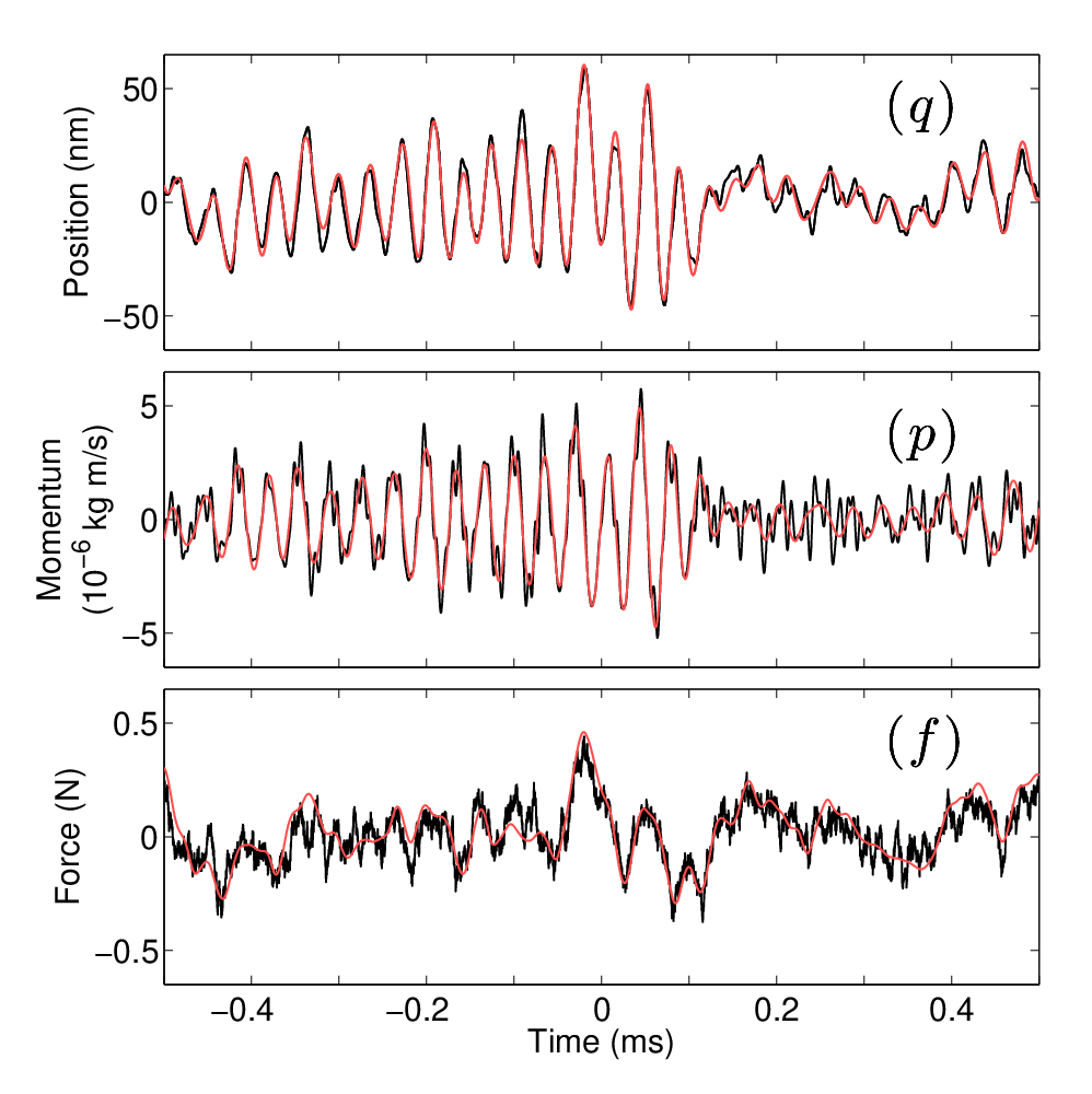
Figure 2 shows one of the time-domain results for the mirror-motion estimation with phase-squeezed states. The black lines are the signals to be estimated (for the evaluation, see Supplemental Material [25]). The external force is an Ornstein-Uhlenbeck process given by Eq. (8). The periodic oscillations of and arise from the mechanical resonance of the PZT-mounted mirror, the frequency of which is rad/s [25]. The red lines are the estimates, which agree well with the signals. This 1 ms long data are obtained with a sampling frequency of 10 MHz, and are repeated 300 times to evaluate the MSEs.

We perform mirror-motion estimation with probe beams in the coherent state and the phase-squeezed state, each with four different amplitudes. Figure 3 shows the dependence of the MSEs of the position, momentum, and external force estimation. Figure 3 shows three key results. First key result: Experimental results agree well with the theoretical predictions (traces i and iii). The small discrepancies may be attributed to the low-frequency noise due to environmental phase drift, and slight changes of the mirror properties (e.g., the resonant frequency) during the experiment. Second key result: The experimental results are close to the waveform QCRBs. In particular, the experimental results for coherent states (green circles) are very close to the coherent-state QCRBs (traces ii). The closeness (i.e., relative differences between the experimental MSEs and the coherent-state QCRBs) is quantified as , , and on average for the position, momentum and force estimates, respectively. The small differences between the prediction curves (traces i) and the coherent-state QCRBs (traces ii) are attributed to the imperfect detection efficiency. The experimental results of squeezed states (red diamonds) are also comparable to the squeezed-state QCRBs (traces iv), although the gaps are larger due to the impurity of the squeezed states. Third key result: The experimental results for squeezed states show clear quantum enhancement, mostly overcoming the coherent-state QCRBs. The quantum enhancements (i.e., relative reduction of MSEs compared to the coherent-state QCRBs) are quantified as and on average for the position and momentum estimates, respectively. The force estimate at the highest probe amplitude is slightly worse than the coherent-state QCRB, which should be due to the low-frequency noise from the environment. Note that we still observe quantum enhancement of the force estimation (except the estimate at the highest probe amplitude), which is quantified as on average.
In conclusion, we have experimentally demonstrated quantum-limited mirror-motion estimation via optical phase tracking. Our experiment reveals that the coherent-state QCRB is almost attainable by our experimental method. Although the squeezed-state QCRB turns out to be more difficult to reach because of the impurity of the squeezed states, quantum enhancement beyond the coherent-state QCRB is clearly observed. These results demonstrate the potential of our theoretical and experimental methods for future quantum metrological applications.
Acknowledgements.
This work was partly supported by PDIS, GIA, G-COE, APSA, FIRST commissioned by the MEXT of Japan, SCOPE program of the MIC of Japan, the Singapore National Research Foundation under NRF Grant No. NRF-NRFF2011-07, and the Australian Research Council projects CE110001029 and DP1094650. The authors would like to thank Hugo Benichi for helpful advice on FPGA digital signal processing. H. Y. acknowledges Shuntaro Takeda for constructive comments on the manuscript.References
- [1] V. B. Braginsky and F. Y. Khalili, Quantum Measurement (Cambridge University Press, Cambridge, 1992).
- [2] H. M. Wiseman and G. J. Milburn, Quantum Measurement and Control (Cambridge University Press, Cambridge, 2010).
- [3] V. Giovannetti, S. Lloyd, and L. Maccone, Science 306, 1330 (2004).
- [4] R. Schnabel, N. Mavalvala, D. E. McClelland, and P. K. Lam, Nature Commun. 1, 121 (2010).
- [5] T. J. Kippenberg and K. J. Vahala, Science 321, 1172 (2008).
- [6] M. Aspelmeyer, S. Gröblacher, K. Hammerer, and N. Kiesel, J. Opt. Soc. Am. B 27, A189 (2010).
- [7] D. Budker and M. Romalis, Nature Phys. 3, 227 (2007).
- [8] H. Katori, Nature Photonics 5, 203 (2011).
- [9] M. A. Taylor, J. Janousek, V. Daria, J. Knittel, B. Hage, H.-A. Bachor, and W. P. Bowen, Nature Photonics 7, 229 (2013).
- [10] C. W. Helstrom, Quantum Detection and Estimation Theory (Academic Press, New York, 1976).
- [11] V. Giovannetti, S. Lloyd, and L. Maccone, Nature Photon. 5, 222 (2011).
- [12] M. Tsang, H. M. Wiseman, and C. M. Caves, Phys. Rev. Lett. 106, 090401 (2011).
- [13] M. Tsang, ArXiv e-prints (2013), arXiv:1301.5733v3 [quant-ph] .
- [14] T. A. Wheatley, D. W. Berry, H. Yonezawa, D. Nakane, H. Arao, D. T. Pope, T. C. Ralph, H. M. Wiseman, A. Furusawa, and E. H. Huntington, Phys. Rev. Lett. 104, 093601 (2010).
- [15] H. Yonezawa, D. Nakane, T. A. Wheatley, K. Iwasawa, S. Takeda, H. Arao, K. Ohki, K. Tsumura, D. W. Berry, T. C. Ralph, H. M. Wiseman, E. H. Huntington, and A. Furusawa, Science 337, 1514 (2012).
- [16] H. M. Wiseman, Phys. Rev. Lett. 75, 4587 (1995).
- [17] D. W. Berry and H. M. Wiseman, Phys. Rev. A 65, 043803 (2002).
- [18] D. W. Berry and H. M. Wiseman, Phys. Rev. A 73, 063824 (2006).
- [19] M. A. Armen, J. K. Au, J. K. Stockton, A. C. Doherty, and H. Mabuchi, Phys. Rev. Lett. 89, 133602 (2002).
- [20] M. Tsang, J. H. Shapiro, and S. Lloyd, Phys. Rev. A 78, 053820 (2008).
- [21] M. Tsang, J. H. Shapiro, and S. Lloyd, Phys. Rev. A 79, 053843 (2009).
- [22] M. Tsang, Phys. Rev. Lett. 102, 250403 (2009a).
- [23] M. Tsang, Phys. Rev. A 80, 033840 (2009b).
- [24] M. Tsang, Phys. Rev. A 81, 013824 (2010).
- [25] See Supplementary Material.
- [26] H. L. Van Trees, Detection, Estimation, and Modulation Theory, Part I. (John Wiley & Sons, New York, 2001).
- [27] Y. Takeno, M. Yukawa, H. Yonezawa, and A. Furusawa, Opt. Express 15, 4321 (2007).
- [28] C. Gardiner and P. Zoller, Quantum noise, Vol. 56 (Springer, 2004).
Supplemental Material for
Quantum-Limited Mirror-Motion Estimation
I Experimental details
In this section, we will describe the experimental details. Figure 4 shows our experimental setup [15]. A continuous-wave Titanium Sapphire laser was used as a light source at 860 nm. Phase squeezed states were generated by an optical parametric oscillator (OPO) of a bow-tie shaped configuration with a periodically polled KTiOPO4 crystal as a nonlinear optical medium [27]. The OPO was driven below threshold by a 430 nm pump beam, generated by another bow-tie shaped cavity that contains a KNbO3 crystal. The free spectral range and the half width at half maximum of the OPO were 1 GHz and 13 MHz respectively. Optical sidebands at 5 MHz were used as a carrier beam generated with acousto-optic modulators [15, 14]. Note that these optical sidebands are within the OPO’s bandwidth. To avoid experimental complexities, the pump power was fixed to 80 mW giving squeezing and anti-squeezing levels of dB and 6.000.15 dB respectively. The effective squeezing factor, , varied from dB to dB according to the probe amplitude. Note that takes into account of the anti-squeezing quadratures mixing in the measurement, which cannot be neglected for relatively high squeezing levels. It is a trade-off between enhancement from the squeezed quadratures and degradation from the anti-squeezed quadratures, revealing an optimal squeezing level [15]. The optimal squeezing level differs for each amplitude , but the difference is minor for our experimental conditions. Since the generated phase squeezed state becomes less robust for higher pumping levels due to the complex locking system, we chose a slightly lower pumping level and did not change it for each . For comparison to phase squeezed states, we also used coherent states as a probe by simply blocking the pump beam.

The mirror mounted on a piezoelectric transducer (PZT) was driven by a signal that follows the Ornstein-Uhlenbeck process. This signal was generated with a random signal generator followed by a low-pass filter with a cutoff frequency of rad/s.
A fraction of the laser beam was used as a local oscillator (LO) beam which was passed through a spatial-mode cleaning cavity (not shown in Fig. 4) to increase mode matching with the probe beam. The probe beam and the LO beam are optically mixed with 1:1 beam splitter for homodyne detection. The efficiency of the detection is shown in Table 1. The homodyne output was demodulated and recorded with an oscilloscope for post processing.
| Photo diode quantum efficiency | 0.99 |
| Interference efficiency (Visibility) | 0.965 (0.982) |
| Propagation efficiency | 0.981 |
| Electrical circuit efficiency (Clearance) | 0.924 (11.2 dB) |
| Overall efficiency | 0.871 |
In the feedback loop, the LO phase is modulated according to the estimated phase. The modulation was performed with a waveguide type electro-optic modulator (EOM). The real-time phase estimate used for feedback was processed with a field programmable gate array (FPGA). The delay of our implemented feedback filter was around 400 ns, which is small enough for our current experimental parameters. Note that we have another low-gain, low-frequency feedback loop to prevent environmental phase drifting.
II Modeling the mirror motion
In this section, we will explain modeling the mirror motion. First, we will consider how to evaluate mass of a PZT-mounted mirror. Then, we will explain transfer function of the PZT-mounted mirror, and the evaluation of true signals to be estimated. Finally we will describe the mirror motion functions.
II.1 Mass of a mirror attached to a PZT
In our experiment, a multilayer PZT (AE0203D04F, NEC/Tokin) of 3.5 mm4.5 mm5.0 mm in size weighing 0.432 g was used. A mirror, 12.7 mm in diameter, 1.5 mm in thickness, weighing 0.444 g was attached to the PZT with an epoxy-based adhesive. The mass of the mirror attached to the PZT was evaluated as follows.
Let the mass of the PZT and mirror be and , respectively. Assume that the mass of the PZT is uniform, and that the displacement is proportional at all points,
| (9) |
Here, the original length of the PZT is , the overall displacement is , and the displacement at point is . Then, the kinetic energy may be calculated as
| (10) |
Hence, we assume that g kg.
II.2 Transfer function of the PZT-mounted mirror
Next, we will focus on modeling the transfer function of the PZT-mounted mirror. The mass-spring-damper model is referred to as the nominal model, which is a simplified model that describes the essence of the targeted system. On the other hand, a model which best describes the targeted system is referred to as the detailed model. The detailed model would be the closest measurable model of the targeted system. We used this detailed model to construct optimal filters and calculate the QCRBs, while we used the nominal model to realize real-time feedback control.

We used a Mach-Zehnder interferometer and a network analyzer to measure the transfer function of the PZT-mounted mirror, , referred to as the detailed model. The black solid lines in Fig. 5 show the measured results. The red dashed lines in Fig. 5 show the fitted transfer function of the nominal model where is the damping coefficient and is the mechanical resonant frequency. The fitted parameters were rad/s and rad/s.
Note that the external force driving the mirror is generated according to the Ornstein-Uhlenbeck process. The cutoff frequency of this process was set to rad/s, which is indicated as a green dot-dashed line in Fig. 5. The nominal model is good enough to construct the real-time feedback filter for the experimental conditions.
II.3 Evaluation of true signals
In order to evaluate estimation errors, we need to know the true position, momentum and external force that are to be estimated (referred to as the target position, target momentum, and target force). We use the full range of the detailed model to calculate these target position , momentum , and external force . In the mirror motion estimation experiment, we record the voltage that drives the PZT-mounted mirror. From , , and the sensitivity of the photo detector V/m, we calculate the target position as
| (11) |
where denotes the (inverse) Fourier transform. We use this result to calculate the target momentum,
| (12) |
The voltage applied to the PZT-mounted mirror is within the linear response range so that the target force may be calculated as
| (13) |
where N/V.
II.4 Mirror motion functions
Mirror motion functions are defined such as ( and ) where a tilde indicates the Fourier transform. The mirror motion functions are necessary to derive the optimal filters and the QCRBs. Note that the definition leads to and .
III Optimal linear filter and least mean square error
In this section, we derive the optimal linear filters which minimize mean square errors (MSEs) [26]. We will explain the position estimate and the least position MSE as an example. The estimates and MSEs for momentum and force can be derived similarly.
First, let’s consider the normalized output of the homodyne detection [17, 15],
| (18) | ||||
| (19) |
Here is the squeezing (anti-squeezing) parameter , is the coherent amplitude of the probe beam, denotes white Gaussian noise with a flat spectral density of , and is a real-time phase estimate used for the feedback control. This homodyne output can also be applied to coherent states by simply putting . Following the quadratic approximation shown in Ref. [15] gives a good approximation of the homodyne output as
| (20) |
Here, is a white Gaussian noise as,
| (21) | ||||
| (22) | ||||
| (23) | ||||
| (24) |
is called the effective squeezing factor [15], which takes into account the anti-squeezed amplitude quadrature as well as the squeezed phase quadrature.
By adding the real-time phase estimate (which is measured in the experiment as well as ) to , we obtain the (modified) measurement result ,
| (25) |
The linear estimate of position, , is given as a weighted sum of this ,
| (26) |
where is a linear position filter. Fourier transform of the estimate is calculated as,
| (27) |
We define a two-time covariance ,
| (28) |
Note that we stick to steady-state so that is determined by only . The Fourier transform of is defined as,
| (29) |
MSE of the position estimation, , is given as as,
| (30) |
Our aim is to derive the filter minimizing and obtain the least .
Let’s focus on because is minimized by minimizing at all the . After some algebra, we find the following:
| (31) |
where is a spectral density defined as . By setting , we obtain the optimal position filter ,
| (32) |
Accordingly, the least MSE is derived as,
| (33) |
The other optimal filters and MSEs for and can be obtained by changing the subscript to or .
The spectral densities () in our experiment are obtained as follows: First, is easily obtained from Eq. (22),
| (34) |
The external force obeys the Ornstein-Uhlenbeck process,
| (35) | ||||
| (36) |
Thus, is given as,
| (37) |
Other spectral densities can be calculated by using the relation . From Eq. (14) we obtain,
| (38) | ||||
| (39) |
IV Photon flux fluctuation
In this section, we will derive the spectral density of the photon flux fluctuation and discuss the validity of the approximation used in the main text, .
In order to calculate the photon flux fluctuation, we use an annihilation operator for an electromagnetic field, , which satisfies the commutation relation [28],
| (40) | ||||
| (41) |
Photon flux and the mean photon flux are given as,
| (42) | ||||
| (43) |
We define the Fourier transform of an annihilation operator,
| (44) |
Note that this definition leads to . The commutation relation in the frequency domain is derived from Eqs. (40) and (41),
| (45) | ||||
| (46) |
Spectral density of is given as,
| (47) | ||||
| (48) |
The mean photon flux is obtained by integrating this spectral density ,
| (49) |
The spectral density of the photon flux fluctuation is calculated as,
| (50) |
To derive , we have to calculate the fourth order moment of an annihilation operator. In our case, however, we use a Gaussian state (phase squeezed state), so the second order moment will suffice to describe .
Let’s assume an annihilation operator of the form,
| (51) | ||||
| (52) |
where is a coherent amplitude, represents the squeezing term ), and are vacuum modes. Here we set the amplitude as a real value without loss of generality. The expression of Eq. (52) is valid for any mean-zero Gaussian states including mixed states (i.e., squeezed thermal states), as long as the coefficient satisfies the following:
| (53) | ||||
| (54) | ||||
| (55) |
Here these equations are imposed by the property of the Fourier transform and the commutation relation (Eqs. (45) and (46)).
To describe the photon flux fluctuation of the squeezed states, it is useful to define the quadrature operators,
| (56) | ||||
| (57) |
Since we set the amplitude as a real value, () is the anti-squeezing (squeezing) quadrature. Photon flux spectrum (except the amplitude contribution), squeezing spectrum and anti-squeezing spectrum (spectral densities of , and ) are given as,
| (58) | ||||
| (59) | ||||
| (60) |
Here squeezing and anti-squeezing spectrum satisfy an uncertainty principle, (). From Eqs. (51) (60), we obtain,
| (61) | ||||
| (62) |
Then, after some algebra, Eq. (50) is rewritten as,
| (63) |
Next, we will assume that the squeezed state has finite bandwidth, and then verify the approximation used in the main text.
Let’s consider the squeezing spectrums of the standard form [27, 15],
| (64) | ||||
| (65) |
where () is the bandwidth of squeezing (anti-squeezing), the second equation ensures that for all when the squeezed state is pure. Here we define the averaged squeezing bandwidth and the squeezing parameters (, ) at the center frequency () as,
| (66) | ||||
| (67) | ||||
| (68) |
In the case of the OPO, corresponds to the half width at half maximum of the OPO.
By inserting Eq. (64) to Eq. (63), we obtain,
| (69) | ||||
| (70) |
where is the mean photon flux of the squeezing ().
If the averaged squeezing bandwidth is much larger than the system parameters, i.e., (: the resonant frequency of the mirror, : the cutoff frequency of the external force), we may assume . Note that we implicitly assume that , which would be justified in our experimental situation as described later. The photon flux fluctuation would be approximated to,
| (71) | ||||
| (72) |
where the parameter ranges from 1 () to 1/4 (). If ,
| (73) |
Let’s consider whether these conditions ( and ) are satisfied under our experimental situation. The experimental parameters are, ( dB), =0.435 ( dB), , , rad/s, and rad/s. The averaged squeezing bandwidth , however, is tricky to determine. As in Ref. [15], we utilize only finite bandwidth around a sideband frequency of 5 MHz. Thus it is not appropriate to define the squeezing bandwidth as an OPO’s bandwidth ( rad/s ). We should consider an effective squeezing bandwidth which is not unnecessarily large, but still satisfies .

Figure 6 shows as a function of the squeezing bandwidth . We also plot experimental amplitude squares 1.02, 1.88, 2.87, 6.24 s-1. In Fig. 6, there is a certain region which satisfies and . For example, let’s set the effective squeezing bandwidth as ten times of the resonant frequency, (). In this case, we obtain s-1 which is still an order smaller than the experimental . Thus we can assume the effective squeezing bandwidth which simultaneously satisfies and . Accordingly we may conclude that the approximation is valid within our experimental conditions.