Framework for maximum likelihood analysis
of neutron decay observables
to resolve the limits of the law
Abstract
We assess the ability of future neutron decay measurements of up to precision to falsify the standard model, particularly the law, and to identify the dynamics beyond it. To do this, we employ a maximum likelihood statistical framework which incorporates both experimental and theoretical uncertainties. Using illustrative combined global fits to Monte Carlo pseudodata, we also quantify the importance of experimental measurements of the energy dependence of the angular correlation coefficients as input to such efforts, and we determine the precision to which ill-known “second-class” hadronic matrix elements must be determined in order to exact such tests.
pacs
11.40.-q, 13.30.Ce, 23.40.-s, 24.80.+yI Introduction
Inspired by the pioneering global fits of the Cabibbo-Kobayashi-Maskawa (CKM) matrix developed by the CKMfitter Group [1, 2] and the UTfit Collaboration [3, 4, 5, 6, 7] for the interpretation of flavor-physics results from the factories and the Tevatron, we outline the prospects for the elucidation of physics beyond the standard model (BSM) via a global fit of neutron decay observables, including the lifetime and the energy-dependence of the angular correlation coefficients. Our global fit, which we term Fitter, employs a maximum likelihood statistical framework which accounts for both experimental and theoretical uncertainties, with the latter arising primarily from the poorly known weak hadronic second-class currents.
The elucidation of a “” law [8, 9] in the mediation of low-energy weak interactions played a crucial role in the rise of the standard model (SM) [10]. A variety of well-motivated SM extensions speak to the possibility of new dynamics at the Fermi scale, which we identify via , and, concomitantly, to tangible departures from the law in low-energy weak processes, be it through scalar or tensor interactions, or right-handed currents. Alternatively, e.g., new, light degrees of freedom could appear and yield violations of the law — if probed at sufficient experimental resolution. At the same time, an ongoing vigorous experimental program for precision measurements of neutron decay observables with cold and ultracold neutrons [11, 12, 13, 14, 15, 16, 17] exists with an overarching goal of realizing bettered assessments of the limits of the SM. The experimental effort focuses on measurements of two general types of observables: angular correlation coefficients, which parametrize the angular correlations between the momenta of the various decay products and/or the spin of the initial state neutron or electron in the differential decay rate, and the neutron lifetime . Of the future experimental plans reviewed in Refs. [11, 12, 13, 14, 15, 16, 17, 18, 19], the claim of ultimate precision rests with the PERC experiment [20], for a sensitivity of up to precision.
The angular correlation coefficients , , , , and [21], of which only , , and are measured to be nonzero [22], describe the distribution in electron and neutrino directions and electron energy in neutron decay. Since the nucleon mass is markedly larger than the neutron-proton mass difference, a recoil expansion of the differential decay rate of the neutron in terms of the ratio of various small energy scales to the nucleon mass is extremely efficient. The , , and correlation coefficients in this order, which we denote with a “” subscript, are functions only of in the SM, where and are the weak axial-vector and vector coupling constants; this is tantamount to the law. Note that for consistency with earlier work [23, 24, 25], we employ a sign convention, so that the sign of the terms in the weak currents are chosen opposite to that of the Particle Data Group [22]. We also assume that is real, which has been established beyond our assumed level of sensitivity in the observables we consider [26, 27]. Thus, extractions of , , and from the measured parameters , , and determine in the SM, which, by itself, is a fundamental parameter of the weak interaction. Using the measured values for and determines and independently. The former, once radiative corrections are applied [28, 29], yields the CKM matrix element . A neutron-based value for [22] is not yet competitive with the result extracted from measurements of the values in superallowed nuclear decays [30, 31]. Such efforts are nevertheless well-motivated in that they are not subject to the nuclear structure corrections which must be applied in the analysis of transitions. We set such prospects aside and focus on the possibility of discovering dynamics beyond the SM through an assessed quantitative violation of the law.
We consider neutron beta decay observables exclusively, though the framework — and fits — we employ can readily be enlarged to encompass all low-energy semileptonic processes involving first-generation quarks. This is possible because we can employ, rather generally, a single, quark-level effective Lagrangian, at leading power in [32, 33], for all such processes [34, 35], where we refer to Ref. [18] for a review. To realize this we need only assume that new physics appears at an energy scale in excess of the scale , crudely that of the and masses. This allows the construction of an effective Lagrangian in terms of operators of mass dimension with [36], where the nonobservation of non-SM invariant operators in flavor physics [37, 7, 2], allows us to impose SM electroweak gauge invariance in its construction. At leading power in , there are then precisely ten dimension-six operators describing the semileptonic decay of the quark. The coefficients of these operators can be determined, or at least constrained, through a global fit of decay observables — in neutrons and nuclei — and of meson decay observables as well. This quark-level description, upon matching to a nucleon-level effective theory [38], yields a one-to-one map to the terms of the effective Hamiltonian constructed by Lee and Yang [39], admitted by Lorentz invariance and the possibility of parity violation [39]. The latter framework is employed in the usual analysis of the angular correlations in beta decay [21]. The construction of the underlying quark-level effective theory allows the inclusion of meson observables on the same footing.
Global fits of the Lee-Yang coefficients have been made to beta decay observables, particularly of the phase-space-integrated angular correlation coefficients [12, 40]. As we develop explicitly, the advantage of the current approach is that we can take theory errors into direct account in the optimization procedure. We focus on the simultaneous fit of the angular correlation coefficients and in neutron decay and of the neutron lifetime to limit the appearance of tensor and scalar interactions from physics BSM, in part because the theory errors in this case are spanned by the ill-known nucleon matrix elements of particular local operators, which presumably and eventually can be computed in QCD using the techniques of lattice gauge theory.
The empirically determined correlation coefficients and neutron lifetime, fixed to some precision, can be used to set limits on new dynamics. In this regard it is natural to focus on the Fierz interference term because it is linear in new physics couplings. That is, it is possible to discover evidence of scalar or tensor interactions, through a measurement of in excess of the level expected in the SM from recoil-order effects [24]. To date there have been no published results for in neutron decay, although several efforts are underway. Searches for scalar and tensor interactions have also been pursued via measurements of the decay electron’s transverse polarizations with respect to the neutron spin [41, 42], though no new experiments of such ilk are currently planned. Information on can be gleaned in different ways. Its presence modifies the shape of the electron energy spectrum in the differential decay rate, and direct searches probe that. It is also subsumed in measurements of the energy dependence of the , , and correlation coefficients [43, 38], so that we wish to consider the additional experimental observables offered by (electron) energy dependence with some care. The latter pathways offer “indirect” access to and require greater statistical control than spectral shape measurements for fixed sensitivity to scalar and tensor interactions. However, they are also less sensitive to systematic errors, both experimental and theoretical. In this first paper we focus on access to scalar and tensor interactions through measurements of , , and , as we now explain.
The description of neutron decay includes contributions from six possible weak hadronic currents which give rise, at recoil order, to energy-dependent expressions for the angular correlation coefficients. However, the most recent extractions of from [44, 45, 46, 47, 48], which yield, at present, the most precise determination of , have assumed the validity of the conserved-vector-current (CVC) hypothesis (i.e., the CVC value for the weak magnetism coupling) and neglected second-class currents. This is certainly reasonable at the current level of experimental precision, although measurements of at the % level of precision are, in principle, sensitive to the weak magnetism coupling, which contributes to the asymmetry at the % level. With the anticipated increased sensitivity to , , and in next-generation experiments, we note that precise measurements of the energy dependence of the and correlations offer the possibility to test CVC and to search for second-class currents independently [25]. In Fitter we fit the energy dependence of the angular correlation coefficients directly and thus need not assume either the validity of the CVC hypothesis or the absence of second-class currents, yielding a framework for a robust test of the validity of the description of neutron decay.
The outline of the remainder of this paper is as follows. First, we review the formalism for the analysis of neutron decay observables in Sec. II. We then briefly review in Sec. III the experimental status of, or limits on, the various SM parameters relevant to our global fit, such as second-class currents. We then describe the maximum likelihood approach to our global fit in Sec. IV, where we discuss the construction of our likelihood function, as well as the inclusion of experimental and theoretical uncertainties. We illustrate the prospects of our global fit with a few numerical examples employing the frequentist, or specifically fit [1, 2], statistical procedure, reserving the use of alternative statistical procedures for later work. We then show examples of the results from Fitter fits to Monte Carlo generated pseudodata in Sec. V under various scenarios, and we quantify via these examples the statistical impact that future improvements in the precision of neutron decay observables should have on the assessment of the validity of the SM. We also discuss the extent to which theoretical uncertainties in the presently poorly known second class contributions limit such assessments, and we can extract from such studies the precision to which they should be established to obviate that impact. Finally, we conclude with a brief summary in Sec. VI.
II Formalism for Neutron -Decay Observables
If we suppose the low-energy, effective weak interaction, employing explicit and degrees of freedom, is mediated by the ten dimension-six operators enumerated by Lee and Yang [39], then the differential decay rate for neutron decay takes the form [21]
| (1) |
where we refer to Ref. [21] for the explicit form of and the correlation coefficients in terms of the parameters of the Lee-Yang Hamiltonian [39], noting Ref. [18] for a discussion of the connection to modern conventions. We use () and () to denote, respectively, the electron’s (antineutrino’s) total energy and momentum, where is the electron endpoint energy, and is the neutron polarization.
The Coulomb corrections to Eq. (1) are also known [49] and modify the expression most notably in terms of a multiplicative Fermi function [50]. The phase-space integrated Fermi function and corrections to it have been studied in great detail [51, 52]; we omit it, as well as the outer radiative correction [53], in the generation of the Monte Carlo pseudodata for our decay correlation studies as we are interested in and , which are accessed through asymmetry measurements for which such effects only lead to a slight modification of the relative statistics (via the spectral shape).
The term is a naively time-reversal-odd observable: a value for in excess of the level attributed to SM final-state interaction effects [54, 55] would reveal the existence of new CP-violating interactions at the Lagrangian level (assuming CPT holds). The current level of experimental precision places stringent constraints on any such new effects [26, 27].
In what follows we report expressions for the correlation coefficients which include the tree-level new physics of the Lee-Yang Hamiltonian and the contributions of the usual terms through recoil order. In realizing this the strong interaction plays an essential role: the matrix elements of the vector and axial-vector currents are described by six distinct form factors. We find it immensely useful to note the quark-level effective theory which underlies the Lee-Yang couplings [34, 38, 35]; it makes clear the separation of the QCD physics which underlies the hadronic matrix element calculation from the nominally higher-energy physics encoded in the effective low-energy constants. As per Refs. [38, 35] we map the Lee-Yang effective couplings with to and note the hadronic matrix elements needed in decay are [56]
| (2) | |||||
| (3) | |||||
| (4) | |||||
| (5) | |||||
where denotes the momentum transfer, , and is the neutron mass. In neutron decay, the -dependent terms are of next-to-next-to-leading order (NNLO) in the recoil expansion, noting and appear in leading order (LO), and hence are of negligible practical relevance. Consequently, we replace, as usual, the form factors with their values at zero momentum transfer. We note is the vector coupling constant given by under CVC; is the weak magnetism coupling constant given by under CVC, noting is the anomalous magnetic moment of the proton (neutron); is the induced scalar coupling constant; is the axial vector coupling constant; is the induced tensor coupling constant; and is the induced pseudoscalar coupling constant. The CVC predictions have SM corrections in NNLO. The contributions of , , , and to the hadronic current are termed first-class currents, whereas those of and are termed second-class currents, due to their transformation properties under -parity [56]. The latter quantities, and , vanish in the SM up to quark mass effects which break flavor symmetry; we discuss their estimated size in Sec. III.
Of particular interest to us are the scalar and tensor interactions, as establishing their existence at current experimental limits would signify the presence of physics BSM. The matching of the quark-level to nucleon-level effective theories at LO in the recoil expansion yields:
| (6) |
where the coefficients are the low-energy constants of the quark-level effective theory of Refs. [38, 35]. We have neglected the matrix elements with in realizing this expression and thus, for consistency, shall neglect the scalar and tensor contribution to recoil order terms in all that follows. Bhattacharya et al. [38] have employed a fit scheme to determine the impact of improved lattice estimates of and on the limits on the quark-level low-energy coeffcients for given experimental sensitivities to .
In unpolarized neutron decay, the unpolarized differential distribution relevant for a measurement of , neglecting terms beyond next-to-leading order in the recoil expansion but accounting for all six possible form factors, is of the form [57]
| (7) | |||||
where is the electron-antineutrino opening angle and . The structure of this expression serves as a de facto definition of and in recoil order. It follows that of Ref. [21] if recoil terms are neglected and is that of Ref. [59] if . Note that in writing the recoil contributions we have neglected terms of . Moreover,
| (8) | |||||
| (9) |
with in the SM, and the kinematic factors , , and are defined according to
| (10) |
The computations of Ref. [58] have been repeated in deriving these forms, and the results are consistent up to the terms [25]. They are also consistent with Ref. [24], as well as with Ref. [59], noting in the latter. These comparisons are all within the context of theory.
We use itself, noting , to characterize the efficacy of the recoil expansion. Both SM and BSM couplings appear in , , and , namely [21]
| (11) | |||||
| (12) | |||||
| (13) |
where we employ Eq. (6).
Our recoil-order expression for the term proportional to appearing within the first set of square brackets in the differential distribution of Eq. (7) is equivalent to the term labeled “” employed in Refs. [60, 38]. However, it should be noted that the second-class currents and yield an additional term which is proportional to . Simply for the sake of notation, we label this term “”, where we then have, in summary,
| (14) |
In polarized decay, the differential distribution relevant to a measurement of is of the form
| (15) | |||||
where is the angle between the momentum of the electron and the polarization of the neutron. Here, too, the structure of this expression follows that of Refs. [59] and [21] in suitable limits and serves as a definition of in recoil order; note that we neglect recoil contributions to , so that “” is the same quantity here and in Eq. (7). The complete expression for can be found in Ref. [57] and is in agreement with Ref. [23]. To LO in the recoil expansion, is of the form
| (16) |
Working to LO in the and terms and to NLO in the terms,
| (17) | |||||
and is of the form
| (18) | |||||
with
| (19) |
Our expressions in the context of theory agree with those of Ref. [24] — and with those of Ref. [59] if .
As a final topic we revisit the computation of the neutron lifetime and focus particularly on the role of recoil-order corrections. In the current state of the art [28, 29], , , and are related by
| (20) |
where in the absence of new physics. Employing and [22] yields a lifetime of s. The numerical value reported in Eq. (20), as per Ref. [29], incorporates an improved treatment of electroweak radiative effects, including certain contributions [28, 29]. Note that the calculation embeds a value of in matching the short- and long-distance radiative corrections [28, 29]. The numerical value also includes the phase space factor which incorporates the Fermi function and various recoil-order terms [51]; many small terms involving hadronic couplings other than and can enter in recoil order. Reference [51] analyzes neutron decay to 0.001% in precision and finds the latter corrections negligible save for the possibility of that from . In that work [51] contributions proportional to are assumed to be strictly zero from CVC, though such can also be engendered by SM isospin violation. We can evaluate the various small contributions to the total decay rate by integrating the terms of Eq. (17) over the allowed phase space of Eq. (15). We denote a contribution relative to that from by , where and are the couplings it contains. Defining , , , and finally
| (21) |
the small contributions to the decay rate, relative to that mediated in LO by , are
| (22) |
where we note the appendix of Ref. [51] for a useful tabulation of the integrals . In our current study, in which we assume that the entire range of possible electron energies is experimentally accessible, both and vanish up to contributions nominally of and in size, both of which are negligible at 0.001% precision. Using the masses reported in Ref. [22], specifically , , and , the remaining terms evaluate to
| (23) |
Using [22] we find . If changes within , we note that changes negligibly at the precision to which we work, so that we can regard as a fixed constant in the optimizations to follow. This particular contribution should already be embedded in the numerical constant of Eq. (20); however, the terms involving second-class currents have not been. To include such small corrections in the lifetime we need only replace with , so that to retain , e.g., we write
| (24) |
It is worth noting that finite experimental acceptance plays an important role in the assessment of the recoil corrections to the lifetime. For example, if the accessible electron kinetic energy were limited to the interval keV from the allowed range of keV, then and would no longer vanish in . The integrals are still analytically soluble and evaluate to and , where we use [22] as well. Taken together, they yield a contribution some 100 times larger than our earlier assessment, which was set by . Including these effects in the manner of Eq. (24), they reduce the determined neutron lifetime for fixed by s to yield s. Such considerations differentiate neutron lifetime experiments which (i) count surviving neutrons from those which (ii) count decay products. The existing tension between the latter, “in beam” experiments and the former, “bottle” experiments [22, 17] — though there is also tension between the results of the most precise bottle experiments [22, 17] — make the observation intriguing. However, the most precise in-beam neutron lifetime experiment [61, 62] counts decay protons, rather than electrons, so that our numerical analysis is not directly relevant. Indeed, in such experiments, there are no threshold effects, and the entire proton recoil spectrum is empirically accessible [61, 62]. On the other hand, experimental concepts which detect the decay electrons have been under development [63, 64].
III Survey of Theoretical Uncertainties
In the SM the corrections to the predictions of the CVC hypothesis, , , and are parametrically known to be of [65] for and of for and . The coupling does not vanish under CVC, but rather from its -parity properties; it, too, is nominally nonzero at .
The CVC hypothesis is assumed (i.e., ) in extracting values for from measured values in superallowed nuclear decay, and the universality of in these decays has been tested to at 68% confidence level (CL) with a concomitant constraint of [30], implying is constrained to only . Direct computation reveals the deviation of from unity to be smaller still [66]. Decay correlation measurements invariably conflate tests of the CVC prediction for the weak magnetism form factor [67] with those which would limit second-class currents; currently the CVC value of is tested to the level of some 6% [12, 68] at 68% CL. We note, however, there has not, to date, been a published measurement of in neutron decay, such as, e.g., could be extracted from the linear energy dependence of , or if is assumed. The second-class couplings and have also not been probed experimentally in neutron decay. The comparison of values in mirror transitions can also test for second-class currents; in that context the weak magnetism form factor does not enter but an isospin-breaking additive correction from the axial form factors can. Such experiments give the strongest empirical constraints on second-class currents [69, 70] although additional theoretical uncertainties enter. A survey of nuclear decay data gives the limit at 90% CL, yielding at 90% CL [71].
Some theoretical studies of exist, particularly in the case of strangeness-changing transitions. A bag model estimate gives [72] in semileptonic transitions. More recently, non-zero second-class currents have been observed in quenched lattice QCD calculations of form factors which appear in the hyperon semileptonic decay , yielding and [73]. Turning to the nucleon sector, we expect these estimates to be suppressed, crudely, by . This makes them nearly compatible in scale with the value for determined using QCD sum rule techniques, [74].
The same lattice study has explored SU(3) breaking in the coupling as well, finding , a result somewhat different from the predictions of common models of SU(3) breaking [73]. Applying a scaling factor of we would suppose that CVC breaking in is no larger than a few percent. It is notable that the experimental limits on , , and are all rather lax with respect to theoretical expectations of CVC breaking and SCC from SM physics.
In what follows we explore the impact of a non-zero , as well as of values of and which are not fixed precisely by the CVC prediction. These form factors all appear in recoil order; the usual first assumption of uncorrelated errors suggests that the impact of these form factors on the potential discovery of BSM physics ought be modest. This turns out to be not so because the fit parameters, rather, are highly correlated, as we shall see.
IV Maximum Likelihood Analysis
IV.1 Construction of the likelihood function
Having reviewed the formalism for neutron decay, the starting point for our maximum likelihood analysis of neutron decay observables is the frequentist fit framework of the CKMfitter Group [1, 2]; in future work we will explore the other analysis schemes outlined by the CKMfitter Group [1, 2] and the UTfit Collaboration [3, 4, 5, 6, 7], such as Bayesian analyses. We review CKMfitter’s fit analysis in sufficient detail to provide sufficient context for the discussion of our global fit. Complete details on the fit statistical framework can, of course, be found in their original papers [1, 2].
Our global fit includes two different types of experimental observables: (i) results for angular correlation coefficients as a function of (binned) electron energy and (ii) the neutron lifetime. We consider each of the bin-by-bin results for the angular correlation coefficients to constitute a separate result. Adopting the notation of the fit framework, we label each of these experimental measurements . Each of them are then compared with a corresponding theoretical calculation of that quantity, . These theoretical calculations are each a function of model parameters, the set of which we denote as . Of these parameters, are experimentally-accessible “free parameters” of the model, the set of which we denote as . The remaining “calculated parameters,” for which there have been no prior experimental measurements and which are not accessible in the current experiments (noting, e.g., second-class currents), must be calculated within the context of the model, subject to various assumptions. The set of these calculated parameters we denote as .
The set of experimental observables includes binned-in-energy measurements of and [where we use the subscripts and to label the particular experiment and the energy bin, respectively] and results for the neutron lifetime, , from different experiments,
| (25) | |||||
These are then to be compared, one-by-one, with a corresponding set of theoretical calculations,
| (26) | |||||
which depend on the set of parameters. Under the SM, the set of parameters would include
| (27) |
though we note that does not appear in decay observables computed through NLO precision. Consequently we set in all that follows; we refer the reader to the reviews of Refs. [75, 76] for information on this quantity. In the next section where we show results from example fits for different scenarios, we define for each scenario which of the parameters are to be considered a free or calculated parameter. We note a subtlety in regards to : if it is a fit parameter, rather than a calculated one, it can be modified by the appearance of a right-handed coupling emergent from physics BSM [38]. Thus the determined value of from a fit of neutron beta decay observables need not be equivalent to the calculated value of . However, present lattice calculations of are of rather poorer precision than empirical determinations. The above sets could, of course, be trivially expanded to accommodate measurements of other observables; for example, the set could include measurements of the neutrino asymmetry and (direct) measurements of the Fierz interference term (via spectral shape measurements), and/or the set could include .
As per the usual prescription [22], we define our function in terms of a likelihood function for the parameter set as
| (28) |
Following the fit framework [1, 2], we define to be the product of an “experimental likelihood” function, , and a “theoretical likelihood” function, ,
| (29) | |||||
The experimental likelihood function is defined in the usual way to be the product of the likelihood functions for each of the experimental results,
| (30) |
where, in the ideal case, the individual likelihood functions are taken to be Gaussian,
| (31) |
where denotes the statistical uncertainty of the th experimental result. Of course, the individual experimental likelihood functions must account for systematic errors, and the formalism for the inclusion of such within the context of the fit framework is described in detail in Refs. [1, 2]. However, a detailed discussion of the impact of experimental systematic errors is beyond the scope of this paper, as the focus of our first paper is on the statistical impact of a global fit and the limitations on such from theoretical uncertainties.
In principle, a theoretical likelihood function could similarly be defined as the product of likelihood functions for each of the calculated parameters,
| (32) |
and under the assumption that the values are Gaussian distributed, the theoretical likelihood would, by definition, contribute to the . Such a formulation might not be appropriate for the treatment of the parameters, for which the underlying probability distributions are certainly not known. However, it may well be possible to bound the value of each parameter on theoretical grounds, such that the parameter may reasonably assume any value over an allowed range of . It would be highly unlikely that the true value of the parameter would fall outside of this range.
Thus, given the lack of knowledge on the underlying distributions of the parameters, the proposal of the fit scheme [1, 2] is to redefine the function so that the theoretical likelihood does not contribute to the , while the parameters are permitted to vary freely within their pre-defined allowed ranges. In particular, the is re-defined to be
| (33) |
where
Thus, under the fit scheme, each of the parameters are bounded, but all possible values of the parameters within their pre-defined ranges are treated equally. That is, the value of is scanned over the available parameter space, while the values of the parameters are permitted to vary freely over their pre-defined ranges at each point in the parameter space. Thus, the central challenge of such an analysis in Refs. [1, 2] is to define the allowed ranges carefully because: (i) the fit results for the parameters can be interpreted as valid only if the “true” values for the parameters fall within the allowed ranges; and (ii) choosing the allowed ranges to be too wide (i.e., too conservative) could mask the discovery of new physics.
After construction of the , a global fit can be then be pursued under two different types of analyses: (i) determining values for the SM parameters; and (ii) assessing the validity of the SM.
IV.2 Determining standard model parameters
Here the goal is neither to assess the validity of the SM nor to search for evidence of new physics. Instead, the SM is assumed to be valid, and the global fit is employed, optimally, to determine values for all of the parameters. In this case, the minimum value of , computed according to Eq. (28), is obtained by allowing all of the parameters to freely vary. The resulting minimum value is denoted . Confidence levels, , on the values of the parameters obtained at are calculated according to
| (34) |
where, as usual,
| (35) |
and Prob(…) denotes the probability for a value of for degrees of freedom.
However, in practice, it may not be possible, or feasible, to determine values for all of the parameters. The parameters, notably the second-class couplings, and , and the induced pseudoscalar coupling , serve as examples. We let denote the subset of parameters for which the goal is to determine confidence levels; the remainder of the parameters are denoted . Note that the set of parameters may not be identical to the set of parameters.
Confidence levels on the parameter set are then determined by first computing at each point in the parameter space the minimal value of the function, , obtained by allowing the parameters to vary. The minimal value of at that point in the parameter space is then computed according to
| (36) |
The confidence levels are then obtained from
| (37) |
IV.3 Assessing the standard model
Under the minimization scheme just described for the determination of SM parameters, the SM is assumed to be valid by definition. In principle, a test statistic for assessing the validity of the SM would be the value of obtained when all of the are varied, where a confidence level on the SM could be defined as
| (38) |
| Input Parameters | |||||||
|---|---|---|---|---|---|---|---|
| Standard Model | PDG: 1.2701 | CVC: | 0 | 0 | 0 | 0 | 0 |
| New Physics | PDG: 1.2701 | CVC: | 0 | 0 | 0 | 0 | |
| Calculated Parameters | |||||||
| Standard Model | 5.83946 | 0 | 885.631 s | ||||
| New Physics | 5.83951 | 885.624 s |
In practice, an assessment of the validity of the SM can be obtained via a Monte Carlo calculation according to the following scheme. Values for the set of experimental results are sampled in the Monte Carlo from their corresponding set of theoretical expressions, , assuming the fitted values for the parameter set. For each set of values, a value is computed, as before, by allowing the parameters to vary. This is repeated, and from this a (normalized) distribution of values, , is constructed. A confidence level for the SM is then deduced from this distribution according to
| (39) |
V Example Fit Scenarios
We now illustrate, via several examples of Fitter fits to Monte Carlo pseudodata, the impact that simultaneous fits to the energy dependence of the and angular correlation coefficients have on an assessment of the validity of the SM and the extent to which theoretical uncertainties can limit such an assessment.
V.1 Monte Carlo data sets and statistics
We generated Monte Carlo pseudodata by sampling the relevant recoil-order differential distributions for measurements of and , Eqs. (7) and (15), respectively, employing the complete expression for in Ref. [57] in the latter case — only the terms of Eq. (17) are appreciably nonzero. We generated two different data sets. The first data set, which we term our “Standard Model” data set, consists of simulated events for a measurement of , and a separate data set consisting of simulated events for a measurement of . Both data sets employ the current Particle Data Group average value for [22] and the CVC value for [22], and assume all of the other small terms are zero, .
The second data set, which we term our “New Physics” data set, again consists of simulated events for a measurement of , and events for a measurement of . This data set is identical to the earlier one, save for the inclusion of a nonzero value for a tensor coupling, namely, , close to the strongest empirical limit on this quantity, which comes from a Dalitz study of radiative pion decay [77, 18]. Specifically, we note the extracted 90% CL limit on [77, 18] can be combined with [38], or , both in the scheme at a renormalization scale of 2 GeV, to yield . The most stringent limit on , which comes from the analysis of nuclear decays [30], is of a comparable magnitude. However, as can be seen from Eq. (13), for approximately equal values of and , is significantly more sensitive to tensor couplings; hence, we have decided to illustrate our methods using a non-zero tensor coupling exclusively. A summary of our input parameters and the resulting values for , , , , and are given in Table 1. Note that we calculate as per Eq. (20), assuming the central value for the superallowed value of [22].
Our pseudodata consists of events, because such is needed for the anticipated level of statistical precision in the most ambitious of the next generation of decay correlation experiments. Specifically, we would be able to determine the value of in an measurement to 0.010% (equivalent to a 0.037% determination of ) and to 0.008% in an measurement (0.032% determination of ). The stated goals on and in the upcoming PERC experiment [20] are to achieve statistical and systematic errors on the level of 0.03%.
The numerical results presented hereafter employ the full energy range (i.e., kinetic energies ). Of course, in a real experiment, the lower energy range will necessarily be in excess of zero due to hardware thresholds and/or analysis cuts. Also, considerations of systematics may limit the upper energy range because energy loss effects become disproportionately more important as the electron energy increases, see, e.g., Refs. [46, 47, 48]. Such details would, of course, be included in a global fit to actual data; the point of this paper is to illustrate the method.
V.2 Examples: Fits to the Standard Model data set
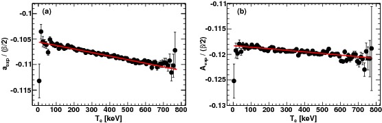
For our first example, we consider fits to the Standard Model data set. As an illustration of our methods, we show our simulated data for and as a function of in Fig. 1, employing 79 10-keV bins from 0–790 keV, as the endpoint is keV. We plot the “experimental asymmetries” and , scaled by the nominal electron-energy dependence of the asymmetries, where the factor of results from the angular integral on a hemisphere. These experimental asymmetries and are calculated from the simulated data in a manner similar to how actual experimental data would be analyzed in a typical “forward/backward” asymmetry measurement (see, e.g., [78]), where
| (40) | |||||
| (41) | |||||
Sensitivity to from and have been previously considered by Refs. [43, 38, 80]. In a real experiment the effects of radiative corrections [79] would have to be removed to interpret in terms of the simple theoretical expressions we employ, noting Eqs. (8) and (18), in our fits. We avoid this now for simplicity, and we are able to do so because said correction incurs no additional hadronic uncertainty. Moreover, for similar reasons we drop the term from our fits as well; they are simply trivially small. The fits shown in Fig. 1 are the result of a simultaneous fit to the and data, in which , noting is shorthand for the complete set of the binned-in-energy results for and , and . We fix to its CVC value and set all second-class couplings to zero, so that vanishes. As a validation of our methods, the fit result for agrees with the input value to within with a , yielding a perfectly acceptable .
Relaxing the assumption that second class currents are zero, we apply the fit scheme to a fit in which , and and comprise the parameter set, which are then permitted to vary simultaneously over some prescribed range, as per the prescription discussed in Sec. IV.2. Of the other parameters, is again fixed to its CVC value, and is fixed to zero. The resulting 68.3% CL on for different assumptions on the permitted theory ranges for and/or are compared in Table 2. Note that we determine a 68.3% CL as per the requirement , where in this case and . Referring to Table 2, unless can be constrained to , theory uncertainties in would limit the precision to which can be extracted from experiments aiming to measure and to the level of 0.03%. Even at this level, the range of the 68.3% CL on is % larger than the case in which second class currents are taken to be exactly zero. In contrast the fits are almost completely insensitive to the value of ; this is because the latter appears only in the terms.
| range | range | Fitted |
|---|---|---|
| Fit | Fitted | Pull | Prob | ||
|---|---|---|---|---|---|
| 1.27056(48) | 0.174(171) | 133.0/156 | 0.91 | ||
| 1.294(40) | 6.7(11.3) | 54.4/77 | 0.98 | ||
| 1.2708(14) | 0.28(65) | 77.8/77 | 0.45 | ||
| Fit | Correlation coefficient | ||||
| 0.97 | |||||
| 1.00 | |||||
| 0.99 | |||||
Alternatively, in the absence of a theory bound on , one could fit directly for and . In what follows we neglect the small contribution, setting , which is reasonable, as we show in Table 2. Results from a fit in which , with no parameters, are shown in Table 3, where the errors on and are defined by , i.e., the 68.3% CL for a joint fit of two free parameters [22]. As one would expect, the error on from a two-parameter simultaneous fit to the data set is a factor of larger than that from a single-parameter fit for alone; and, it is worth noting that can be determined from such a fit to . However, what is more interesting are the errors on and extracted from a fit to the data set alone: the error on is a factor of larger than that from a single-parameter fit for alone, and the error on is of . The origin of this effect is clear: appears in only in the expansion for , Eq. (8), namely via the combination . Therefore, and are directly correlated in a small recoil-order term in , with only the fitted value of ultimately limiting the range and, hence, the and errors. In Table 3, we also show the “Pull,” which we define as for a parameter . In the event of asymmetric errors, we average the two errors to form . For completeness, the correlation coefficients from the fits are also given. Thus, this example succinctly illustrates the necessity of a stringent theoretical bound on the value of for an interpretation of measurements in the context of an assessment of the structure of the SM.
As a final example of fits to our Standard Model data set, we consider the implications of CVC breaking on the value of the weak magnetic form factor , by defining and under different assumptions on the permitted theory range for . The results are summarized in Table 4. As can be seen there, the impact of a % breaking on is comparable to an uncertainty in .
| range | Fitted |
|---|---|
| CVC exact | 1.27009(8) |
| % | 1.27009(9) |
| % | 1.27011(11) |
| % | 1.27016(15) |
V.3 Examples: Fits to the New Physics data set
As our second example, we consider fits to the New Physics data set. As can be seen in Table 1, the values of and in the New Physics data set differ from their values in the Standard Model data set by only 0.004% and 0.005%, respectively. Therefore, the impact of any new physics from scalar and tensor interactions on the measured values of and will be via a “dilution” to the experimental asymmetries and from a non-zero Fierz term appearing in the denominators of Eqs. (40) and (41), respectively. Accordingly, we now expand our parameter set to include .
Results from a single parameter fit in which only and an empty parameter set are shown in Table 5. As can be seen, these fits still yield excellent values for ; however, not surprisingly, there are significant pulls on the fitted values for from the input value. The origin of these pulls can be easily understood (and, indeed, was first noted by Ref. [38]) by inspecting the functional forms for and in terms of and . For small , with or , whereas the slope of the dependence of and is negative in and nearly linear; the contributions to and from and are of the same sign and slope. Therefore, the presence of a non-zero would not result in poor values in fits to the and energy dependence.
| Fit | Fitted | Pull | Prob | |
|---|---|---|---|---|
| 1.27115(8) | 153.6/157 | 0.56 | ||
| 1.27135(13) | 75.0/78 | 0.57 | ||
| 1.27103(10) | 74.7/78 | 0.59 |
| and | ||||
|---|---|---|---|---|
| Fit | Fitted | Pull | Prob | |
| 151.9/157 | 0.60 | |||
| 75.0/78 | 0.58 | |||
| 73.9/78 | 0.61 | |||
| and | ||||
| Fit | Fitted | Pull | Prob | |
| 151.4/157 | 0.61 | |||
| 74.8/78 | 0.58 | |||
| 71.8/78 | 0.68 | |||
Next, we again consider the implications of theoretical uncertainties in and as relevant for an extraction of in the presence of new physics. The parameter set still includes only, while now the parameter set includes and , which are then permitted to vary over a particular range. The resulting 68.3% confidence levels on extracted from a simultaneous fit to the , as well as to the individual or , New Physics data set, for different theory ranges on and are compared in Table 6. It is interesting to note that the effects of new physics in an measurement considered in isolation could potentially be obscured by second class currents, whereas there is less of an effect for an measurement considered in isolation or in a combined fit to and data. This effect derives from the manner in which appears in .
| Fit | Fitted | Fitted | Prob | |
|---|---|---|---|---|
| 1.27011(65) | 147.5/156 | 0.67 | ||
| 1.27052(113) | 73.8/77 | 0.58 | ||
| 1.27014(86) | 72.2/77 | 0.63 | ||
| Fit | Correlation coefficient | |||
| 0.98 | ||||
| 0.99 | ||||
| 0.98 | ||||
Results from the two-parameter fits, with and an empty parameter set, are summarized in Table 7. It is worth noting that a combined fit at this level of precision has the potential to constrain at 68.3% CL to the level of , although such a fit would also offer significantly less (by a factor of ) less sensitivity to . For completeness, we also list the correlation coefficients for these fits. Finally, we perform fits with and , with and permitted to vary over different particular ranges. The results of these fits, which demonstrate the impact that uncertainties in and have on the allowed parameter space, are shown in Fig. 2. Indeed, as one can see, the allowed parameter space is broadened significantly by the inclusion of theoretical uncertainties in and . As per our analysis reported in Table 2 we note the uncertainty in is of greater impact.

V.4 Example: Impact of the neutron lifetime to an assessment of the SM
Finally, we consider the impact that future measurements of the neutron lifetime to a precision of 0.1 s, considered together with measurements of the and angular correlation coefficients to a precision of %, will have on an assessment of the validity of the structure of the SM. We illustrate this within the context of our New Physics data set. To do so, we expand our data set to , where we take to be a single data point whose value is the calculated value of s for the parameters of the New Physics data set, as per Table 1, and consider various uncertainties in .
| error (s) | Prob | |
|---|---|---|
| 1.00 | 155.1/158 | 0.55 |
| 0.50 | 159.3/158 | 0.45 |
| 0.25 | 174.3/158 | 0.17 |
| 0.20 | 183.8/158 | 0.078 |
| 0.15 | 200.9/158 | 0.011 |
| 0.10 | 233.0/158 | |
| 0.07 | 263.4/158 |
| error (s) | Prob | |
|---|---|---|
| 1.00 | 154.3/157 | 0.55 |
| 0.50 | 158.0/157 | 0.46 |
| 0.25 | 171.1/157 | 0.21 |
| 0.20 | 179.5/157 | 0.11 |
| 0.15 | 194.5/157 | 0.023 |
| 0.10 | 222.6/157 | |
| 0.07 | 249.1/157 | |
| 1.00 | 154.4/157 | 0.54 |
| 0.50 | 158.3/157 | 0.46 |
| 0.25 | 172.1/157 | 0.19 |
| 0.20 | 180.9/157 | 0.093 |
| 0.15 | 196.7/157 | 0.017 |
| 0.10 | 226.3/157 | |
| 0.07 | 254.3/157 |
| error (s) | Prob | |
|---|---|---|
| 1.00 | 152.7/157 | 0.58 |
| 0.50 | 155.0/157 | 0.53 |
| 0.25 | 163.3/157 | 0.35 |
| 0.20 | 168.6/157 | 0.25 |
| 0.15 | 178.0/157 | 0.12 |
| 0.10 | 195.7/157 | 0.019 |
| 0.07 | 212.5/157 | 0.0021 |
| 1.00 | 152.9/157 | 0.58 |
| 0.50 | 155.9/157 | 0.51 |
| 0.25 | 166.5/157 | 0.29 |
| 0.20 | 173.3/157 | 0.18 |
| 0.15 | 185.4/157 | 0.060 |
| 0.10 | 208.1/157 | |
| 0.07 | 229.6/157 |
| error (s) | Prob | |
|---|---|---|
| 1.00 | 152.1/157 | 0.60 |
| 0.50 | 153.0/157 | 0.58 |
| 0.25 | 154.3/157 | 0.55 |
| 0.20 | 154.7/157 | 0.54 |
| 0.15 | 155.0/157 | 0.53 |
| 0.10 | 155.3/157 | 0.52 |
| 0.07 | 155.4/157 | 0.52 |
| 1.00 | 152.4/157 | 0.59 |
| 0.50 | 154.3/157 | 0.55 |
| 0.25 | 158.6/157 | 0.45 |
| 0.20 | 160.3/157 | 0.41 |
| 0.15 | 162.2/157 | 0.37 |
| 0.10 | 164.3/157 | 0.33 |
| 0.07 | 165.6/157 | 0.30 |
We then perform a simultaneous fit to the New Physics data set in which , i.e., with only a single free parameter. We use the CVC value for and set to zero. As we have already noted, a simultaneous fit to the data set only yields excellent values for — albeit, with significant pulls on the fitted values for . The neutron lifetime is relatively insensitive to new scalar or tensor physics, because such new physics only enters quadratically in the parameter, noting Eq. (20). Therefore, we would expect a simultaneous fit to an data set in the presence of new scalar and tensor interactions to return a poor value for . Indeed, the results of such an analysis are shown in Table 8, where we show the fitted values for , the from the fit, and the probability for that value, for different assumed experimental errors on the lifetime. As can be seen, the probability for the validity of the SM, which we quantify via the statistic , as per Sec. IV.3, in the presence of new tensor physics at the level of would become if the neutron lifetime were measured to s or better in concert with % measurements of and . Under this scenario, a precision in the neutron lifetime of 0.07 s would yield a probability of , which is slightly more stringent than the requirement for a result, i.e., a probability of .
Finally we turn to an examination of the impact of a non-zero second-class coupling on the ability to falsify the law of the SM. It has been the usual procedure to ignore certain recoil corrections in the determination of , as per Eq. (20), but we expect that a non-zero value of could be important in this context, so that we include the recoil correction in , as per Eq. (24), as well. We perform a simultaneous fit to the New Physics data set in which and , where is permitted to vary over different particular ranges, with equal to its CVC value and . The empirical limits on are markedly weaker than the existing direct theoretical estimate, noting [74] with [22], so that we perform simultaneous fits using in the following ranges: , , and . The fit results, as well as the determined abilities to falsify the SM, as a function of the error in the determined neutron lifetime, are shown for these ranges of in Tables 9, 10, and 11, respectively. Nonzero values of impact the ability to falsify the SM in every case, and the inclusion of the recoil corrections to are also of importance. In the last case, in which , the ability to falsify the SM with improving precision in the neutron lifetime has been completely eroded. Evidently it is important to determine to the greatest accuracy possible in order to be able to falsify the law of the SM.
VI Summary and Conclusions
In summary, we have developed a maximum likelihood statistical framework, which we term Fitter, in which we make simultaneous fits to various neutron decay observables. Although a number of global fits to decay data have previously been developed [12, 40], the novel approach embedded in our technique is that simultaneous fits to the energy dependence of the angular correlation coefficients allow for a robust test of the validity of the structure of the SM in the presence of theoretical uncertainties, whereas fits based on integral quantities do not. To our knowledge ours is the first study of the quantitative ability to falsify the SM and particularly the law, after the manner of Refs. [1, 2, 3, 4, 5, 6, 7], in the context of neutron beta decay observables.
Our study has consisted of fits to the and angular correlation coefficients, as well as to the value of the neutron lifetime. We believe that studies of the angular correlation coefficient, as well as of through the electron energy spectrum in decay, will offer important complementary information; and such, as well as any additional, concomitant theoretical uncertainties, can be incorporated in our analysis framework as well. In our current study we have focused on the role of second-class current contributions, most notably on the impact of a non-zero coupling, on the ability to identify physics BSM. In the course of developing our analysis procedure, we have discovered that certain recoil effects to the neutron lifetime, contrary to the usual view [51], can have an impact on our fit results. Moreover, the precise form of the recoil corrections depends on experimental details, revealing that the corrections change with a finite experimental acceptance, such as in experiments which extract a value of the lifetime from measurements of the decay electrons and/or protons. Such considerations warrant further detailed study.
We have explicitly shown that it is possible to discover physics BSM, at significance, in neutron decay observables using experiments which are currently planned or under construction. This is subject to the following conditions; namely, that (i) tensor interactions are not much smaller than the constraint which emerges from the Dalitz analysis of pion radiative decay [77, 18], (ii) the value of can be sharply restricted, and (iii) results of 0.03% precision can be realized for and , in concert with a sub- determination of the neutron lifetime. In our study we have assumed that , so that using [38] and noting , this would be commensurate with the appearance of physics BSM at an energy scale of at least [36]. We note that existing direct limits on tensor couplings from nuclear decay are much weaker than those from radiative pion decay [18]; perhaps new physics effects could be different in pion and neutron decays. We note, however, that under the assumption that BSM effects appear at energies in excess of such effects can only occur from operators beyond mass-dimension six and ought be suppressed. Our current analysis framework is also suitable to the discovery of new scalar interactions as well.
We have shown that theoretical uncertainties in can mitigate the gains made in falsifying the SM through the inclusion of precision results. We thus advocate for a determination of using lattice gauge theory techniques; we suppose that lattice measurements of and in neutron decay would be useful, too. These considerations are quite independent of how information on is determined.
Acknowledgements.
S.G. is supported in part by the Department of Energy Office of Nuclear Physics under Grant No. DE-FG02-96ER40989. B.P. is supported in part by the Department of Energy Office of Nuclear Physics under Grant No. DE-FG02-08ER41557.References
- [1] A. Höcker, H. Lacker, S. Laplace, and F. Le Diberder, Eur. Phys. J. C 21, 225 (2001).
- [2] J. Charles, A. Höcker, H. Lacker, S. Laplace, F. R. Le Diberder, J. Malclès, J. Ocariz, M. Pivk, and L. Roos, Eur. Phys. J. C 41, 1 (2005).
- [3] M. Ciuchini, E. Franco, L. Giusti, V. Lubicz, and G. Martinelli, Nucl. Phys. B 573, 201 (2000).
- [4] M. Ciuchini, V. Lubicz, G. D’Agostini, E. Franco, G. Martinelli, F. Parodi, P. Roudeau, and A. Stocchi, J. High Energy Phys. 07 (2001) 013.
- [5] M. Bona et al. [UTfit Collaboration], J. High Energy Phys. 07 (2005) 028.
- [6] M. Bona et al. [UTfit Collaboration], J. High Energy Phys. 10 (2006) 081.
- [7] M. Bona et al. [UTfit Collaboration], J. High Energy Phys. 03 (2008) 049.
- [8] R. P. Feynman and M. Gell-Mann, Phys. Rev. 109, 193 (1958).
- [9] E. C. G. Sudarshan and R. e. Marshak, Phys. Rev. 109, 1860 (1958).
- [10] L. H. Hoddeson, (Ed.), L. Brown, (Ed.), M. Riordan, (Ed.) and M. Dresden, (Ed.), The Rise of the standard model: Particle physics in the 1960s and 1970s (Cambridge University Press, Cambridge, 1997).
- [11] J. S. Nico and W. M. Snow, Annu. Rev. Nucl. Part. Sci. 55, 27 (2005).
- [12] N. Severijns, M. Beck, and O. Naviliat-Cuncic, Rev. Mod. Phys. 78, 991 (2006).
- [13] H. Abele, Prog. Part. Nucl. Phys. 60, 1 (2008).
- [14] J. S. Nico, J. Phys. G 36, 104001 (2009).
- [15] D. Dubbers and M. G. Schmidt, Rev. Mod. Phys., 83, 1111 (2011).
- [16] N. Severijns and O. Naviliat-Cuncic, Annu. Rev. Nucl. Part. Sci. 61, 23 (2011).
- [17] F. E. Wietfeldt and G. L. Greene, Rev. Mod. Phys. 83, 1173 (2011).
- [18] V. Cirigliano, S. Gardner, and B. Holstein, Prog. Part. Nucl. Phys. 71, 93 (2013).
- [19] M. González-Alonso and O. Naviliat-Cuncic, arXiv:1304.1759 [hep-ph].
- [20] D. Dubbers, H. Abele, S. Baessler, B. Maerkisch, M. Schumann, T. Soldner, and O. Zimmer, Nucl. Instrum. Meth. A 596, 238 (2008).
- [21] J. D. Jackson, S. B. Treiman, and H. W. Wyld, Jr., Phys. Rev. 106, 517 (1957).
- [22] J. Beringer et al. (Particle Data Group), Phys. Rev. D 86, 010001 (2012).
- [23] I. Bender, V. Linke, and H. J. Rothe, Z. Phys. 212, 190 (1968).
- [24] B. R. Holstein, Rev. Mod. Phys. 46, 789 (1974) [Erratum-ibid. 48, 673 (1976)].
- [25] S. Gardner and C. Zhang, Phys. Rev. Lett. 86, 5666 (2001).
- [26] H. P. Mumm et al., Phys. Rev. Lett. 107, 102301 (2011).
- [27] T. E. Chupp et al., Phys. Rev. C 86, 035505 (2012).
- [28] A. Czarnecki, W. J. Marciano, and A. Sirlin, Phys. Rev. D 70, 093006 (2004).
- [29] W. J. Marciano and A. Sirlin, Phys. Rev. Lett. 96, 032002 (2006).
- [30] J. C. Hardy and I. S. Towner, Phys. Rev. C 79, 055502 (2009).
- [31] I. S. Towner and J. C. Hardy, Rep. Prog. Phys. 73, 046301 (2010).
- [32] W. Buchmuller and D. Wyler, Nucl. Phys. B 268, 621 (1986).
- [33] B. Grzadkowski, M. Iskrzynski, M. Misiak, and J. Rosiek, JHEP 1010, 085 (2010).
- [34] V. Cirigliano, J. Jenkins, and M. González-Alonso, Nucl. Phys. B 830, 95 (2010).
- [35] V. Cirigliano, M. González-Alonso, and M. L. Graesser, JHEP 1302, 046 (2013).
- [36] T. Appelquist and J. Carazzone, Phys. Rev. D 11, 2856 (1975).
- [37] G. Isidori, Y. Nir, and G. Perez, Ann. Rev. Nucl. Part. Sci. 60, 355 (2010).
- [38] T. Bhattacharya, V. Cirigliano, S. D. Cohen, A. Filipuzzi, M. González-Alonso, M. L. Graesser, R. Gupta, and H.-W. Lin, Phys. Rev. D 85, 054512 (2012).
- [39] T. D. Lee and C. -N. Yang, Phys. Rev. 104, 254 (1956).
- [40] G. Konrad, W. Heil, S. Baeßler, D. Počanić, and F. Glück, arXiv:1007.3027.
- [41] A. Kozela et al., Phys. Rev. Lett. 102, 172301 (2009).
- [42] A. Kozela et al., Phys. Rev. C 85, 045501 (2012).
- [43] F. Glück, I. Joo, and J. Last, Nucl. Phys. A 593, 125 (1995).
- [44] H. Abele et al., Phys. Rev. Lett. 88, 211801 (2002).
- [45] D. Mund et al., Phys. Rev. Lett. 110, 172502 (2013).
- [46] J. Liu et al., Phys. Rev. Lett. 105, 181803 (2010).
- [47] B. Plaster et al., Phys. Rev. C 86, 055501 (2012).
- [48] M. Mendenhall et al., Phys. Rev. C 87, 032501(R) (2013).
- [49] J. D. Jackson, S. B. Treiman, and H. W. Wyld, Jr., Nucl. Phys. 4, 206 (1957).
- [50] E. Fermi, Z. Phys. 88, 161 (1934).
- [51] D. H. Wilkinson, Nucl. Phys. A377, 474 (1982).
- [52] D. H. Wilkinson, Nucl. Instrum. Meth. A 404, 305 (1998).
- [53] A. Sirlin, Phys. Rev. 164, 1767 (1967).
- [54] C. G. Callan and S. B. Treiman, Phys. Rev. 162, 1494 (1967).
- [55] S. Ando, J. A. McGovern, and T. Sato, Phys. Lett. B 677, 109 (2009).
- [56] S. Weinberg, Phys. Rev. 112, 1375 (1958).
- [57] C. Zhang, Ph.D. thesis, University of Kentucky, 2001 (unpublished).
- [58] D. R. Harrington, Phys. Rev. 120, 1482 (1960).
- [59] S. M. Bilen’kiĭ, R. M. Ryndin, Ya. A. Smorodinskiĭ, and T.-H. Ho, Sov. Phys. JETP 37, 1241 (1960).
- [60] V. P. Gudkov, G. L. Greene, and J. R. Calarco, Phys. Rev. C 73, 035501 (2006).
- [61] M. S. Dewey, D. M. Gilliam, J. S. Nico, F. E. Wietfeldt, X. Fei, W. M. Snow, G. L. Greene and J. Pauwels et al., Phys. Rev. Lett. 91, 152302 (2003).
- [62] J. S. Nico, M. S. Dewey, D. M. Gilliam, F. E. Wietfeldt, X. Fei, W. M. Snow, G. L. Greene and J. Pauwels et al., Phys. Rev. C 71, 055502 (2005).
- [63] P. R. Huffman et al., Nature (London) 403, 62 (2000).
- [64] C. R. Brome et al., Phys. Rev. C 63, 055502 (2001).
- [65] M. Ademollo and R. Gatto, Phys. Rev. Lett. 13, 264 (1964).
- [66] N. Kaiser, Phys. Rev. C 64, 028201 (2001).
- [67] M. Gell-Mann, Phys. Rev. 111, 362 (1958).
- [68] T. Sumikama, K. Matsuta, T. Nagatomo, M. Ogura, T. Iwakoshi, Y. Nakashima, H. Fujiwara, and M. Fukuda et al., Phys. Rev. C 83, 065501 (2011).
- [69] K. Minamisono, K. Matsuta, T. Minamisono, T. Yamaguchi, T. Sumikama, T. Nagatomo, M. Ogura, and T. Iwakoshi et al., Phys. Rev. C 65, 015501 (2001).
- [70] K. Minamisono, T. Nagatomo, K. Matsuta, C. D. P. Levy, Y. Tagishi, M. Ogura, M. Yamaguchi, and H. Ota et al., Phys. Rev. C 84, 055501 (2011).
- [71] D. H. Wilkinson, Eur. Phys. J. A 7, 307 (2000).
- [72] J. F. Donoghue and B. R. Holstein, Phys. Rev. D 25, 206 (1982).
- [73] S. Sasaki and T. Yamazaki, Phys. Rev. D 79, 074508 (2009).
- [74] H. Shiomi, Nucl. Phys. A 603, 281 (1996).
- [75] T. Gorringe and H. W. Fearing, Rev. Mod. Phys. 76, 31 (2004).
- [76] V. Bernard, L. Elouadrhiri, and U.-.G. Meißner, J. Phys. G 28, R1 (2002).
- [77] M. Bychkov, D. Pocanic, B. A. VanDevender, V. A. Baranov, W. H. Bertl, Y. .M. Bystritsky, E. Frlez, and V. A. Kalinnikov et al., Phys. Rev. Lett. 103, 051802 (2009).
- [78] B. Plaster et al., Nucl. Instrum. Methods Phys. Res. A 595, 587 (2008).
- [79] R. T. Shann, Nuovo Cim. A 5, 591 (1971).
- [80] K. P. Hickerson, Ph.D. thesis, California Institute of Technology, 2013 (unpublished).