A complete topological invariant for braided magnetic fields

Berger (1988) Berger, M.A.defines ${\cal A}$ as a ‘‘field line helicity’’,helicity!field line or limiting magnetic helicityhelicity in an infinitesimal flux tube around a single magnetic field line. Since our domain is magnetically open, we define a gauge invariant relative helicityhelicity!relative (Berger & Field, 1984; Finn & Antonsen, 1985) Berger, M.A.Field, G.B.Finn, J.H.Antonsen, T.M.relative to the reference field ${\bf B}^{\rm ref}=\nabla\times{\bf A}^{\rm ref}$. Assuming (4), the relative helicity may be written

$$H_{r}=\int_{V}({\bf A}+{\bf A}^{\rm ref})\cdot({\bf B}-{\bf B}^{\rm ref})\,\mathrm{d}^{3}x=\int_{V}{\bf A}\cdot{\bf B}\,d^{3}x-\int_{V}{\bf A}^{\rm ref}\cdot{\bf B}^{\rm ref}\,\mathrm{d}^{3}x.$$

(9)

The last term is a constant (call it $H^{\rm ref}$) which depends only on the choice of reference field. For the first term, let $x_{0}$ be the footpoint of the field line through $x=(\rho,\psi,z)$, so that $x=f(x_{0};z)$. Changing coordinates gives

	$\displaystyle H_{r}-H^{\rm ref}$	$\displaystyle=\int_{V}{\bf A}(x)\cdot{\bf B}(x)\,\mathrm{d}^{3}x,$		(10)
		$\displaystyle=\int_{V}{\bf A}\big(f(x_{0};z)\big)\cdot{\bf B}\big(f(x_{0};z)\big)\frac{B_{z}(x_{0})}{B_{z}\big(f(x_{0};z)\big)}\mathrm{d}^{2}x_{0}\mathrm{d}z,$		(11)
		$\displaystyle=\int_{D_{0}}{\cal A}(x_{0})B_{z}(x_{0})\,\mathrm{d}^{2}x_{0}.$		(12)

Thus we see that ${\cal A}$ represents the helicity per field line.

It is insightful to derive Lemma 2 by interpreting ${\cal A}$ as an action in a Hamiltonian system.Hamiltonian system Suppose we parametrise a magnetic field line in terms of its length $l$ as ${\bf x}(l)$, and think of the topological flux function as a functional,

$${\cal A}(x_{0})=\int_{x_{0}}^{F(x_{0})}{\bf A}({\bf x})\cdot\frac{\mathrm{d}{\bf x}}{\mathrm{d}l}\,\mathrm{d}l.$$

(15)

Then Cary & Littlejohn (1983) Cary, J.R.Littlejohn, R.G.point out that extremising ${\cal A}$ for given ${\bf A}$ and fixed end-points gives the path of the field line ${\bf x}(l)$ through the domain. To see this, note that the Euler-Lagrange equations are

$$\frac{\partial L}{\partial x_{j}}-\frac{\mathrm{d}}{\mathrm{d}l}\left(\frac{\partial L}{\partial(\partial x_{j}/\partial l)}\right)=0.$$

(16)

In our case, the Lagrangian is $L={\bf A}\cdot({\mathrm{d}{\bf x}}/{\mathrm{d}l})$, so

$$\frac{\partial A_{i}}{\partial x_{j}}\frac{\partial x_{i}}{\partial l}-\frac{\partial x_{i}}{\partial l}\frac{\partial A_{j}}{\partial x_{i}}=0,$$

(17)

which is equivalent to

$$(\nabla\times{\bf A})\times\frac{\mathrm{d}{\bf x}}{\mathrm{d}l}=0.$$

(18)

Hence $\mathrm{d}{\bf x}/\mathrm{d}l$ is everywhere parallel to ${\bf B}$, and ${\bf x}(l)$ is a magnetic field line.

In fact, it is well known that the equations of the magnetic field lines are a Hamiltonian system. To show this, we follow Cary & Littlejohn (1983) Cary, J.R. Littlejohn, R.G.and change the gauge of ${\bf A}$ so as to write the action explicitly in the canonical form of a Hamiltonian system. A gauge transformation ${\bf A}\rightarrow{\bf A}+\nabla\chi$ changes the integrand (the Lagrangian) to $L+\mathrm{d}\chi/\mathrm{d}l$ and also changes the integral (the action ${\cal A}$), but leaves the Euler-Lagrange equations unchanged. If we set $A_{\rho}=0$ everywhere in space, then ${\bf A}\cdot\,\mathrm{d}{\bf x}=A_{\psi}h_{\psi}\,\mathrm{d}\psi+A_{z}h_{z}\,\mathrm{d}z$. Making the identifications $p\leftrightarrow A_{\psi}(\rho,\psi,z)h_{\psi},q\leftrightarrow\psi,t\leftrightarrow z,H\leftrightarrow-A_{z}(\rho,\psi,z)h_{z}$, our action becomes

$${\cal A}=\int_{x_{0}}^{F(x_{0})}\left(p\frac{\mathrm{d}q}{\mathrm{d}t}-H(p,q,t)\right)\,\mathrm{d}t,$$

(19)

which is a 1 degree-of-freedom Hamiltonian system in canonical form. The generalised coordinate is $\psi$, the generalised momentum is $A_{\psi}h_{\psi}$, and the Hamiltonian is $-A_{z}h_{z}$. Time is the $z$-direction, so our Hamiltonian is, in general, time dependent.

The gauge where $A_{\rho}=0$ everywhere may be called a canonical gauge since it renders the Hamiltonian system in canonical form. For Theorem 1 it is sufficient that ${\bf n}\times{\bf A}|_{\partial V}$ be in canonical gauge, so in practice we restrict the gauge of ${\bf A}^{\rm ref}$ to be canonical, i.e. $A_{\rho}^{\rm ref}=0$. The gauge $A_{\rho}=0$ is equivalent to writing ${\bf B}$ in the form ${\bf B}=\nabla(A_{\psi}h_{\psi})\times\nabla\psi+\nabla(A_{z}h_{z})\times\nabla z$ (Boozer, 1983; Yoshida, 1994). Boozer, A.H.Yoshida, Z.

Given that ${\cal A}$ is the action in a Hamiltonian system, we can use known properties of Hamiltonian systems. Let $f_{z}$ be the “height-$z$” mapping of our field line system, defined by $f_{z}(x_{0})=f(x_{0};z)$. This mapping must preserve magnetic flux. In terms of differential forms, $f_{z}^{*}\omega-\omega=0$, where $\omega=B_{z}h_{\rho}h_{\psi}\,\mathrm{d}\rho\wedge\mathrm{d}\psi$. Every Hamiltonian system preserves such a symplectic form $\omega$. But notice that

$$\omega=\left(\frac{\partial}{\partial\rho}\big(A_{\psi}h_{\psi}\big)-\frac{\partial}{\partial\psi}\big(A_{\rho}h_{\rho}\big)\right)\,\mathrm{d}\rho\wedge\mathrm{d}\psi=\mathrm{d}\alpha$$

(20)

where $\alpha=A_{\psi}h_{\psi}\,\mathrm{d}\psi+A_{\rho}h_{\rho}\,\mathrm{d}\rho$. The primitive $\alpha$ is called the canonical/Liouville 1-form.

Assume now that ${\bf A}$ is in canonical gauge as above, so that $\alpha=A_{\psi}h_{\psi}\,\mathrm{d}\psi$. Then Lemma 2 follows from the following argument (Haro, 1998). Haro, A.In canonical coordinates, Hamilton’s equations have the form

$$\dot{p}=-\frac{\partial H}{\partial q},\quad\dot{q}=\frac{\partial H}{\partial p}.$$

(21)

If we define the Hamiltonian vector field ${\bf x}(t)\equiv(x^{q},x^{p})=(\dot{q},\dot{p})$, then Hamilton’s equations may be succinctly written (Marsden & Ratiu, 1994) Marsden, J.E.Ratiu, T.S.in terms of $\alpha$ as

$$i_{\bf x}\,\mathrm{d}\alpha=-\mathrm{d}H.$$

(22)

By the definition of the Lie derivative (Marsden & Ratiu, 1994, Theorem 4.3.1 of ), using Cartan’s magic formula, and the fact that differentials and pull-backs commute, we have

$$\frac{d}{ds}(f_{s}^{*}\alpha)=f_{s}^{*}{\cal L}_{{\bf x}(s)}\alpha=f_{s}^{*}\big(i_{{\bf x}(s)}\,\mathrm{d}\alpha+\mathrm{d}i_{{\bf x}(s)}\alpha\big)=\mathrm{d}f_{s}^{*}\big(i_{{\bf x}(s)}\alpha-H\big).$$

(23)

Integrating both sides from $s=0$ to $s=z$ yields the desired formula

$$f_{z}^{*}\alpha-\alpha=\mathrm{d}\Big(\int_{0}^{z}f_{s}^{*}\big(i_{{\bf x}(s)}\alpha-H\big)\,\mathrm{d}s\Big).$$

(24)

Taking $z=1$ in this expression and recognising (19) gives

$$F^{*}\alpha-\alpha=\mathrm{d}\Big(\int_{0}^{1}f_{z}^{*}\big(p\dot{q}-H\big)\,\mathrm{d}z\Big)=\mathrm{d}\Big(\int_{0}^{1}\big(p\dot{q}-H\big)\circ f_{z}\,\mathrm{d}z\Big)=\mathrm{d}{\cal A},$$

(25)

which is Lemma 2.

To show that Lemma 2 holds even in non-canonical gauge, suppose that $F^{*}\alpha-\alpha=\mathrm{d}{\cal A}$ for some ${\bf A}$. Under the change of gauge ${\bf A}\rightarrow{\bf A}+\nabla\chi$, we find $\alpha\rightarrow\alpha+\mathrm{d}\chi$, so

$$F^{*}\alpha-\alpha\quad\rightarrow\quad F^{*}\alpha-\alpha+\mathrm{d}(F^{*}\chi-\chi)=\mathrm{d}(\cal A+F^{*}\chi-\chi).$$

(26)

But this is precisely $\mathrm{d}{\cal A}$ in the new gauge (Section 2), so if the Lemma holds in one gauge it holds in any gauge.gauge transformation

We already know that ${\cal A}$ is a necessary condition for topological equivalence, because it is an ideal invariant. But we can also see this from Lemma 2. Assuming $\widetilde{F}=F$, it follows that

$$\mathrm{d}\widetilde{\cal A}=\widetilde{F}^{*}\alpha-\alpha=F^{*}\alpha-\alpha=\mathrm{d}{\cal A},$$

(27)

so that $\widetilde{\cal A}$ and ${\cal A}$ differ by at most an overall constant. But since $\widetilde{F}|_{\partial D_{0}}=F_{\partial D_{0}}$ (with the same winding number) we must have $\widetilde{\cal A}={\cal A}$ (see Figure 3).

To prove the converse—that ${\cal A}$ is a sufficient condition for topological equivalence—assume that ${\cal A}=\widetilde{\cal A}$ and define the mapping $G=\widetilde{F}\circ F^{-1}$. Then, using Lemma 2,

	$\displaystyle G^{*}\alpha-\alpha$	$\displaystyle=(F^{-1})^{*}\circ\widetilde{F}^{*}\alpha-\alpha$		(28)
		$\displaystyle=(F^{-1})^{*}(\alpha+\mathrm{d}{\cal A})-\alpha$		(29)
		$\displaystyle=(F^{-1})^{*}\alpha-\alpha+(F^{-1})^{*}\mathrm{d}{\cal A}$		(30)
		$\displaystyle=(F^{-1})^{*}\alpha-(F^{-1})^{*}\circ F^{*}\alpha+(F^{-1})^{*}\mathrm{d}{\cal A}$		(31)
		$\displaystyle=(F^{-1})^{*}(\alpha-F^{*}\alpha)+(F^{-1})^{*}\mathrm{d}{\cal A}$		(32)
		$\displaystyle=-(F^{-1})^{*}\mathrm{d}{\cal A}+(F^{-1})^{*}\mathrm{d}{\cal A}$		(33)
		$\displaystyle=0.$		(34)

Now we determine the possible mappings $G:D_{1}\rightarrow D_{1}$ satisfying $G^{*}\alpha=\alpha$, which Haro (1998); Haro (2000) Haro, A.calls “actionmorphisms”. If $\alpha$ is in the canonical gauge $A^{\rm ref}_{\rho}=0$, then the possible mappings $G$ that preserve $\alpha$ are known (Marsden & Ratiu, 1994, Proposition 6.3.2) Marsden, J.E.Ratiu, T.S.to take the form of cotangent lifts

$$G(q,p)=\left(T(q),\frac{p}{T^{\prime}(q)}\right)$$

(35)

where $T$ is a diffeomorphism. Since $\partial D_{0}$ is not a line of constant $q(\equiv\psi)$, it follows from our assumption $\widetilde{F}|_{\partial D_{0}}=F|_{\partial D_{0}}$ that $T(q)=q$ and hence that $G_{q}=q$, $G_{p}=p$. We see that $G_{\psi}=\psi$. Recalling that $p=A^{\rm ref}_{\psi}h_{\psi}$, we note in canonical gauge that $B_{z}>0$ implies that $\partial p/\partial\rho>0$. It follows that the coordinate transformation from $(\rho,\psi)$ to $(p,q)$ has non-zero Jacobian, and hence that $G_{\rho}=\rho$. So $G={\rm id}$ and therefore $\widetilde{F}=F$. ∎

1. 1.

   If $\alpha$ is not in the canonical gauge, then $G$ need not take the form of a cotangent lift. Indeed, the nature of the actionmorphisms appears to depend on the gauge of $\alpha$. For suppose that $G^{*}\alpha-\alpha=0$ for some $\alpha$. Then after a gauge transformation $\alpha\rightarrow\alpha+\mathrm{d}\chi$ we find

   $$G^{*}(\alpha+\mathrm{d}\chi)-(\alpha+\mathrm{d}\chi)=\mathrm{d}(G^{*}\chi-\chi)\neq 0$$

   (36)

   so that $G$ is no longer an actionmorphism in the new gauge.gauge transformation

2. 2.

   Notice that the property of whether or not two magnetic braids are topologically equivalent does not depend on the choice of reference field. This choice is arbitrary; all that matters is that the same reference field is used to compute both ${\cal A}$ and $\widetilde{\cal A}$. On the other hand, the nature of differences in ${\cal A}$ between two inequivalent braids may depend on the choice of reference: this is an issue for future investigation.

Take standard cylindrical coordinates $\rho=r$ and $\psi=\phi$, so that the scale factors are $h_{\rho}=h_{z}=1$, $h_{\psi}=r$. Consider the magnetic braid

$${\bf B}={\bf e}_{z}+\sqrt{2}r\,e^{-r^{2}/2-z^{2}/4}{\bf e}_{\phi}$$

(37)

which consists of a localised toroidal “flux ring” in a uniform background field (Wilmot-Smith et al., 2009). Wilmot-Smith, A.L.Hornig, G.Pontin, D.I.For this field the field lines are

$$f_{r}(r,\phi;z)=r,\qquad f_{\phi}(r,\phi;z)=\sqrt{2\pi}\,e^{-r^{2}/a^{2}}\Big({\rm erf}(z/2)-{\rm erf}(z_{0}/2)\Big)+\phi,$$

(38)

and taking $z_{0}\rightarrow-\infty$, $z\rightarrow\infty$ in (37), the field line mapping is

$$F_{r}(r,\phi)=r,\qquad F_{\phi}(r,\phi)=2\sqrt{2\pi}\,e^{-r^{2}/2}+\phi.$$

(39)

A vector potential in the appropriate gauge is

$${\bf A}=\frac{r}{2}{\bf e}_{\phi}+\sqrt{2}\,e^{-r^{2}/2-z^{2}/4}{\bf e}_{z}.$$

(40)

Since $A_{z}\approx 0$ on all boundaries to high accuracy, the corresponding reference is ${\bf A}^{\rm ref}=(r/2){\bf e}_{\phi}$, giving ${\bf B}^{\rm ref}={\bf e}_{z}$. One can then compute the topological flux function analytically, finding

$${\cal A}(r,\phi)=\sqrt{2\pi}(r^{2}+2)\,e^{-r^{2}/2}.$$

(41)

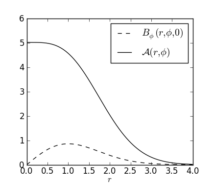
Notice that $\partial{\cal A}/\partial r=-\sqrt{2\pi}r^{3}\,e^{-r^{2}/2}$ and $\partial{\cal A}/\partial\phi=0$. In this case $\alpha=(r^{2}/2)\,\mathrm{d}\phi$ and we can verify that

$$\Big(F^{*}\alpha\Big)(r,\phi)=\frac{F_{r}^{2}}{2}\left(\frac{\partial F_{\phi}}{\partial r}\,\mathrm{d}r+\frac{\partial F_{\phi}}{\partial\phi}\,\mathrm{d}\phi\right)=\frac{r^{2}}{2}\left(-2\sqrt{2\pi}r\,e^{-r^{2}/2}\,\mathrm{d}r+\mathrm{d}\phi\right)$$

(42)

so that indeed $F^{*}\alpha-\alpha=\mathrm{d}{\cal A}$.

Suppose now that the flux ring is displaced from the origin and centred at $(r=1,\phi=0)$. Then the new vector potential is

$${\bf A}=\frac{r}{2}{\bf e}_{\phi}+\sqrt{2}\exp\left(-\frac{(r\cos\phi-1)^{2}+(r\sin\phi)^{2}}{2}-\frac{z^{2}}{4}\right){\bf e}_{z}.$$

(43)

This is not topologically equivalent to the original example, so ${\cal A}$ must differ. One might expect that the ${\cal A}$ distribution would simply be translated, but Figure 5(a) shows that this is not the case: the profile of ${\cal A}$ within the disturbed region is no longer symmetric about the ring centre. This reflects the fact that ${\cal A}$ is a global quantity: it counts not just the horizontal flux of the ring itself, but how it is linked with the reference field ${\bf B}^{\rm ref}={\bf e}_{z}$. In (43), the reference field is asymmetrical with respect to the position of the flux ring.

This may be understood using the following alternative formula for ${\cal A}$ on the cylinder. Yeates & Hornig (2013) Yeates, A.R.Hornig, G.show that ${\cal A}(x_{0})$ is the average pairwise linking number between the field line $f(x_{0};z)$ and all other field lines $f(y_{0};z)$. The linking numberlinking number in this context (Berger, 1988) Berger, M.A.is the integral

$$c_{x_{0},y_{0}}=\frac{1}{2\pi}\int_{-8}^{8}\frac{\mathrm{d}\theta_{x_{0},y_{0}}(z)}{\mathrm{d}z}\,\mathrm{d}z,$$

(44)

where $\theta_{x_{0},y_{0}}(z)$ is the orientation of the line connecting $f(x_{0};z)$ and $f(y_{0};z)$ in the plane at height $z$. It is proved by Yeates & Hornig (2013) Yeates, A.R.Hornig, G.that

$${\cal A}(x_{0})=\int_{D_{0}}c_{x_{0},y_{0}}B_{z}(y_{0})\,\mathrm{d}^{2}y_{0}.$$

(45)

As an aside, notice that equation (45) gives a formula to compute ${\cal A}$ directly from ${\bf B}$ without needing to know ${\bf A}$.

The asymmetry in Figure 5(a) arises due to differing $c_{x_{0},y_{0}}$ for different field lines $f(x_{0};z)$ through the flux ring. To see this, consider two field lines $f(x_{0};z)$ passing through the ring, but starting on opposite sides (Figures 5b and 5c). The contours show $c_{x_{0},y_{0}}$ as a function of $y_{0}$ for each of these $x_{0}$. For $y_{0}$ within the ring itself, the $c_{x_{0},y_{0}}$ contours are the same in each case up to rotation, so these points make the same contribution to the integral (45). But for most $y_{0}$ outside the ring, $c_{x_{0},y_{0}}$ has the opposite sign in Figure 5(b) compared to Figure 5(c), because of the field line direction $f_{y}(x_{0};z)<0$ in Figure 5(b) while $f_{y}(x_{0};z)>0$ in Figure 5(c). Furthermore, since $c_{x_{0},y_{0}}$ is opposite in sign on the left and right of the ring, and since there is a larger area to the left of the ring, the net contributions to (45) from $y_{0}$ outside the ring differ in each case. This explains the asymmetry. In Section 5.1, the area to the left and right of the ring was the same, hence the symmetric ${\cal A}$ profile.

\ack

The work was supported by STFC Grant ST/G002436/1 to the University of Dundee. We thank J. B. Taylor, J.-J. Aly and P. Boyland for useful suggestions.

References

- Berger (1986) Berger, M. A. 1986 Topological invariants of field lines rooted to planes. Geophys. Astrophys. Fluid Dyn. 34, 256–281.
- Berger (1988) Berger, M. A. 1988 An energy formula for nonlinear force-free magnetic fields. Astron. Astrophys. 201, 355–361.
- Berger & Field (1984) Berger, M. A. & Field, G. B. 1984 The topological properties of magnetic helicity. J. Fluid Mech. 147, 133–148.
- Berger & Prior (2006) Berger, M. A. & Prior, C. 2006 The writhe of open and closed curves. J. Phys. A: Math. Theor. 39, 8321–8348.
- Boozer (1983) Boozer, A. H. 1983 Evaluation of the structure of ergodic fields. Phys. Fluids 26, 1288–1291.
- Brown et al. (1999) Brown, M. R., Canfield, R. C. & Pevtsov, A. A. (ed.) 1999 Magnetic Helicity in Space and Laboratory Plasmas, Washington. AGU.
- Candelaresi & Brandenburg (2011) Candelaresi, S. & Brandenburg, A. 2011 Decay of helical and nonhelical magnetic knots. Phys. Rev. E 84, 01646.
- Cary & Littlejohn (1983) Cary, J. R. & Littlejohn, R. G. 1983 Noncanonical hamiltonian mechanics and its application to magnetic field line flow. Annal. Phys. 151, 1–34.
- Finn & Antonsen (1985) Finn, J. H. & Antonsen, T. M. 1985 Magnetic helicity: What is it and what is it good for? Comments Plasma Phys. Contr. Fusion 9, 111–126.
- Frankel (1997) Frankel, T. 1997 The Geometry of Physics. CUP, Cambridge.
- Haro (1998) Haro, A. 1998 The primitive function of an exact symplectomorphism. PhD thesis, Universitat de Barcelona, Barcelona.
- Haro (2000) Haro, A. 2000 The primitive function of an exact symplectomorphism. Nonlinearity 13, 1483–1500.
- Marsden & Ratiu (1994) Marsden, J. E. & Ratiu, T. S. 1994 Introduction to Mechanics and Symmetry. Springer-Verlag, New York.
- Morrison (2000) Morrison, P. J. 2000 Magnetic field lines, hamiltonian dynamics, and nontwist systems. Phys. Plasmas 7, 2279–2289.
- Reale (2010) Reale, F. 2010 Coronal loops: Observations and modeling of confined plasma. Living Rev. Solar Phys. 7, 5.
- Taylor (1986) Taylor, J. B. 1986 Relaxation and magnetic reconnection in plasmas. Rev. Mod. Phys. 58, 741–763.
- Wilmot-Smith et al. (2009) Wilmot-Smith, A. L., Hornig, G. & Pontin, D. I. 2009 Magnetic braiding and parallel electric fields. Astrophys. J. 696, 1339–1347.
- Woltjer (1958) Woltjer, L. 1958 A theorem on force-free magnetic fields. Proc. Nat. Acad. Sci. 44, 489–491.
- Yeates & Hornig (2011) Yeates, A. R. & Hornig, G. 2011 A generalized flux function for three-dimensional magnetic reconnection. Phys. Plasmas 18, 102118.
- Yeates & Hornig (2013) Yeates, A. R. & Hornig, G. 2013 Unique topological characterization of braided magnetic fields. Phys. Plasmas 20, 012102.
- Yeates et al. (2010) Yeates, A. R., Hornig, G. & Wilmot-Smith, A. L. 2010 Topological constraints on magnetic relaxation. Phys. Rev. Lett. 105, 085002.
- Yoshida (1994) Yoshida, Z. 1994 A remark on the hamiltonian form of the magnetic-field-line equations. Phys. Plasmas 1, 208–209.