Structural Analysis of Combustion Mechanisms

Journal: Chemical Engineering Science

J. Tóth Email: jtoth@math.bme.hu Address: Department of Analysis, Budapest University of Technology and Economics, Egry J. u. 1., Budapest, Hungary, H-1111 Address: Laboratory for Chemical Kinetics of the Department of Physical Chemistry, Eötvös Loránd University, Pázmány P. sétány 1/A., Budapest, Hungary, H-1117 Note: Partially supported by the Hungarian National Scientific Foundation, No. 84054 and No. 84060. Note: This work is connected to the scientific program of the "Development of quality-oriented and harmonized R+D+I strategy and functional model at BME" project. This project is supported by the New Széchenyi Plan (Project ID: TÁMOP-4.2.1/B-09/1/KMR-2010-0002). Note: Partially supported by the COST Action CM901: Detailed Chemical Kinetic Models for Cleaner Combustion. Corresponding author: Corresponding author A. L. Nagy Email: nagyal@math.bme.hu Address: Department of Stochastics, Budapest University of Technology and Economics, Egry J. u. 1., Budapest, Hungary, H-1111 Note: Partially supported by the Hungarian National Scientific Foundation, No. 84054 and No. 84060. Note: Partially supported by the COST Action CM901: Detailed Chemical Kinetic Models for Cleaner Combustion. Note: The results discussed below are supported by the grant TÁMOP-4.2.2.B-10/1–2010-0009. I. Gy. Zsély Email: zselyigy@gmail.com Address: Laboratory for Chemical Kinetics of the Department of Physical Chemistry, Eötvös Loránd University, Pázmány P. sétány 1/A., Budapest, Hungary, H-1117 Note: Partially supported by the Hungarian National Scientific Foundation, No. 84054 and No. 84060. Note: Partially supported by the COST Action CM901: Detailed Chemical Kinetic Models for Cleaner Combustion.

Abstract

$39$ detailed mechanisms for combustion of hydrogen, carbon monoxide and methanol are investigated using ReactionKinetics, a Mathematica based package. The obtained results in most cases do not depend on the choice of reaction rate coefficients, the methods only use the underlying sets of reaction steps, thus the results are robust and general in a certain sense. These investigations can be used before or in parallel with usual numerical investigations, such as pathway analysis, sensitivity analysis, parameter estimation or simulation.

The considered hydrogen mechanisms shared 90% of common reaction steps. The CO combustion mechanisms show a larger variety both in species and in reaction steps. There exist only a few methanol combustion mechanisms; the big differences between them shows that the modelling community is only at the very beginning of exploring this process.

The package and the methods may be useful for automatic mechanism generations, testing, comparing and reduction of mechanisms as well, especially in the case of large systems.

Keywords:

combustion, kinetics, mathematical modeling , Mathematica , computational chemistry , graphs of reactions.

1 Introduction

The reaction steps of hydrogen and carbon monoxide combustion form a central part of the high temperature combustion of all hydrocarbons and oxygenates, see e.g. Reed [1997]. Also, hydrogen is an important fuel itself for different applications (e.g. rocket propulsion) and in the context of a carbon-free economy as well as of safety issues. In the recent years, there has been an increased interest in studying the combustion of fuel mixtures consisting of carbon monoxide and hydrogen, referred to as "wet CO" or syngas. These fuels can be produced from coal and biomass via gasification, and are considered to be a promising option towards cleaner combustion technologies for power generation. Oxygenated organic compounds have been proposed as alternative fuels in order to improve the fuel properties and reduce particulates and $\text{NO}{\vphantom{\text{X}}}_{\vphantom{\text{2}}\smash[t]{\text{x}}}^{\vphantom{\smash[t]{\text{2}}}\hphantom{\text{x}}\text{}}$ emissions. Methanol, the most simple alcohol, is one of the most important oxygenated additives due to its high oxygen content and the lack of C–C bonds.

In the present paper we investigate the combustion of hydrogen, carbon monoxide and methanol: three phenomena important both from theoretical and practical points of view in combustion.

The approach we use is absolutely structural in the sense that none of the results depend on the values of the rate coefficients (cf. Beck [1970]). We might say that we are going to discover possibilities instead of quantitatively dealing with individual mechanisms. To put it another way, we are going to raise questions to be answered by the chemist, rather than answering them.

In a previous paper we presented a Mathematica based program package called ReactionKinetics [Nagy et al., 2012] aimed at symbolic and numerical treatment of chemical mechanisms. The package is especially useful when the numbers of species and reaction steps are larger than to allow manual investigations, i.e. if one has dozens or even thousands of species and reaction steps. After the publication of the previous version we made the package capable of reading CHEMKIN files by CHEMKINImport, added dozens of new functions such as e.g.

1.

CHEMKINExport,
2.

MaxFHJWeaklyConnectedComponents,
3.

MinFHJWeaklyConnectedComponents,
4.

MaxFHJStronglyConnectedComponents,
5.

MinFHJStronglyConnectedComponents,
6.

FilterReactions,

and made the package compatible with Version $9$ of Mathematica.

The structure of our paper is as follows. In Section 2 the mechanisms to be investigated are described. Results are shown in Section 3. The necessary mathematical background is relegated to the Appendix.

Finally, two electronic supplements are added. Firstly, a Mathematica notebook showing all the details of the calculations which may be really useful for those interested in combustion modeling but of minor interest for the general audience. Some of the resulting figures are also given there. The calculations can be reproduced by using the package itself. It can be downloaded from the following page:

http://www.math.bme.hu/~jtoth/CES2013.

The data can either be collected from the original authors, or from our database to be built in the near future. Secondly, we also attach the (very long) PDF manuscript of our notebook which allows to passively follow what we have done, but this version does not need the Mathematica program.

2 Selected mechanisms of combustion of hydrogen, carbon monoxide and methanol

The simplest chain branching combustion reaction, the oxidation of hydrogen is already a much more complex system than the Mole and Robertson reactions discussed in the Appendix. It is a common misconception that the chemistry of these low-order systems is well understood. However, Zsély, I. Gy. et al. [2013] showed recently in a comprehensive mechanism comparison paper that this is not the case. The description of the experimental data is still not satisfactory and some of the recently published reaction mechanisms perform worse than older ones. Similar comparison was done by Olm et al. [2013] for the oxidation of carbon monoxide. In this work we utilize the mechanism collection of these papers, but focus on the structural differences of the mechanisms. By extending the investigations to some detailed methanol mechanisms we show that the suggested formal mathematical handling is still applicable for even larger kinetic systems. The phenomena are more and more complex as we proceed from hydrogen through carbon monoxide to methanol. Correspondingly, the mechanisms are larger and more and more diverse.

3 On the structure of the selected combustion mechanisms

Even the simplest mechanisms for combustion usually contain dozens of species and of reaction steps, therefore we can only show selected parts of the results here, e.g. Volpert graphs of the investigated reactions are not shown here as the figures themselves are not useful, they can only be used for calculating the Volpert indices. However, we have shown the Volpert graphs together with Volpert indices for two simple reactions in the Appendix.

3.1 Hydrogen

As a starting point the basic data of the investigated mechanisms are presented in Tables 1 and 2.

Table 1: Basic data of the investigated hydrogen combustion mechanisms I.

Mechanism	Reference	$M$	$R$	$\delta=N-L-S$
Ahmed2007	Ahmed et al. [2007]	8	38	$29-11-6=12$
Burke2012	Burke et al. [2012]	8	38	$31-12-6=13$
CRECK2012	Healy et al. [2010]	8	37	$29-11-6=12$
Dagaut2003	Dagaut et al. [2003]	8	42	$31-12-6=13$
Davis2005	Davis et al. [2005]	8	40	$31-12-6=13$
GRI30	Smith et al. []	8	40	$31-12-6=13$
Hong2011	Hong et al. [2011]	8	40	$31-12-6=13$
Keromnes2013	Kéromnès et al. [2013]	9	42	$32-12-7=13$
Konnov2008	Konnov [2008]	8	42	$31-12-6=13$
Li2007	Li et al. [2007]	8	38	$31-12-6=13$

Table 2: Basic data of the investigated hydrogen combustion mechanisms II.

Mechanism	Reference	$M$	$R$	$\delta=N-L-S$
NUIG2010	Healy et al. [2010]	8	38	$31-12-6=13$
OConaire2004	Ó Conaire et al. [2004]	8	38	$31-12-6=13$
Rasmussen2008	Rasmussen et al. [2008a]	8	40	$31-12-6=13$
SanDiego2011	Combustion Research [2011]	8	42	$31-12-6=13$
SaxenaWilliams2006	Saxena & Williams [2006]	8	42	$31-12-6=13$
Starik2009	Starik et al. [2010]	9	52	$41-16-7=18$
Sun2007	Sun et al. [2007]	8	40	$31-12-6=13$
USC2007	Wang et al. [2007]	8	40	$31-12-6=13$
Zsely2005	Zsély, I. Gy. et al. [2005]	8	42	$31-12-6=13$

Number of species, $M$: All mechanisms contains the same (core) set of species: H, $\text{H}{\vphantom{\text{X}}}_{\vphantom{\text{2}}\smash[t]{\text{2}}}^{\vphantom{\smash[t]{\text{2}}}\hphantom{\text{2}}\text{}}$ , $\text{H}{\vphantom{\text{X}}}_{\vphantom{\text{2}}\smash[t]{\text{2}}}^{\vphantom{\smash[t]{\text{2}}}\hphantom{\text{2}}\text{}}\text{O}$ , OH, $\text{H}{\vphantom{\text{X}}}_{\vphantom{\text{2}}\smash[t]{\text{2}}}^{\vphantom{\smash[t]{\text{2}}}\hphantom{\text{2}}\text{}}\text{O}{\vphantom{\text{X}}}_{\vphantom{\text{2}}\smash[t]{\text{2}}}^{\vphantom{\smash[t]{\text{2}}}\hphantom{\text{2}}\text{}}$ , $\text{HO}{\vphantom{\text{X}}}_{\vphantom{\text{2}}\smash[t]{\text{2}}}^{\vphantom{\smash[t]{\text{2}}}\hphantom{\text{2}}\text{}}$ , $\text{O}{\vphantom{\text{X}}}_{\vphantom{\text{2}}\smash[t]{\text{2}}}^{\vphantom{\smash[t]{\text{2}}}\hphantom{\text{2}}\text{}}$ , O. The Keromnes2013 mechanism, formally, contains $h\nu$ as a species, but this is only a description for the photoexcitation in a photochemical reaction step.

This mechanism is the only one which contains the excited OH species (OHEX) to describe some ignition delay experiments better.

There is another mechanism (Starik2009) which contains an additional species, ozone. It is quite unique to include this species in a reaction mechanism intended to be used for the description of combustion processes.
Number of reaction steps, $R$: The number of reaction steps, $R$ , varies between 37 and 44, except Starik2009, where this number is 52. Thus—as C. K. Law reported in his comprehensive review paper [Law, 2007]—the number of reactions is approximately 5 times larger than the number of species (except the mentioned case).
Deficiency, $\delta$: The number of complexes, $N$ , varies between 29 and 32, except Starik2009, where this number is 41. The number of weakly connected components is either 11 or 12, except again Starik2009, where this number is 16. The preliminary data suggest that Starik2009 is structurally richer than the other mechanisms.

The deficiencies are large, neither the zero deficiency theorem, nor the one deficiency theory can be applied.
Weak reversibility and acyclicity: None of the reactions have an acyclic Volpert graph, as all the reactions, except in CRECK2012, are fully reversible. Accordingly, all the reactions are weakly reversible, except again CRECK2012, which has a single irreversible step: $\text{H}{\vphantom{\text{X}}}_{\vphantom{\text{2}}\smash[t]{\text{2}}}^{\vphantom{\smash[t]{\text{2}}}\hphantom{\text{2}}\text{}}\text{O}{\vphantom{\text{X}}}_{\vphantom{\text{2}}\smash[t]{\text{2}}}^{\vphantom{\smash[t]{\text{2}}}\hphantom{\text{2}}\text{}}$ ${}+{}$ O ${}\mathrel{\mathop{\makebox[0.0pt]{\rightarrow\displaystyle}}\limits}{}$ $\text{HO}{\vphantom{\text{X}}}_{\vphantom{\text{2}}\smash[t]{\text{2}}}^{\vphantom{\smash[t]{\text{2}}}\hphantom{\text{2}}\text{}}$ ${}+{}$ OH.

3.1.1 Representations of mechanism classes

From our—let us emphasize: structural—point of view not all the mechanisms in Tables 1 & 2 are different, one has classes with exactly the same structure if the values of reaction rate coefficients are disregarded. (To put it another way: the underlying complex chemical reaction is the same.) The classes are shown in Fig. 1.

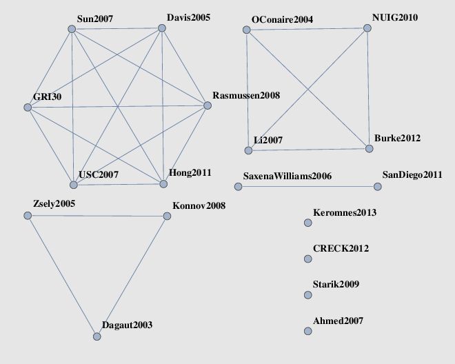
Refer to caption — Figure 1: Classes of hydrogen combustion mechanisms. Mechanisms with the same structure are connected with an edge of the graph

During mechanism development one of the first steps is the decision of which species should be included in the mechanism. After this, the reaction steps and the best possible (to the best knowledge of the authors) set of parameters are selected. This last step, the assignment of the rate parameters forms the largest part of a mechanism development work. However, we have to keep it in mind that the parameter set corresponds to the previously fixed structure of the model. Therefore, it is important to compare the mechanisms from the point of view of their structures. Figure 1 is a demonstrative example that the currently published hydrogen combustion mechanisms are different not at the level of the parameters, but already in their general structures (i.e. the reaction steps underlying in the mechanism). It is interesting to see that a significant number of reaction mechanisms in this collection kept the structure of the old GRI1999. It is also interesting, that when the mechanisms are updated most of the authors do not modify their structures (see the reaction mechanisms coming from the same research group, e.g. SaxenaWilliams2006 and SanDiego2011, or Li2007 and Burke2012, or OConaire2004 and NUIG2010). Clinging to potentially outdated structures can be one of the possible pitfalls in mechanism development. The structural relationship the OConaire2004, Li2007, NUIG2010 and Burke2012 is obvious, as they are based on some older reaction mechanisms of Dryer’s group [Mueller et al., 1999].

However, this finding allows us to choose a single mechanism from the classes, and we remind the reader that from now on Davis2005 also represents GRI30, Hong2011, Rasmussen2008, Sun2007, USC2007; Burke2012 also represents Li2007, NUIG2010, OConaire2004; and Dagaut2003 also represents Konnov2008 and Zsely2005.
SanDiego2011 also represents SaxenaWilliams2006; whereas each of Ahmed2007, CRECK2012, Keromnes2013 and Starik2009 form a separate class. The representatives have been selected by the caprice of the alphabet.

Given that the initial species in the case of hydrogen combustion mechanisms are $\text{H}{\vphantom{\text{X}}}_{\vphantom{\text{2}}\smash[t]{\text{2}}}^{\vphantom{\smash[t]{\text{2}}}\hphantom{\text{2}}\text{}}$ and $\text{O}{\vphantom{\text{X}}}_{\vphantom{\text{2}}\smash[t]{\text{2}}}^{\vphantom{\smash[t]{\text{2}}}\hphantom{\text{2}}\text{}}$ , the Volpert indices of the species are displayed in Tables 3, 4, 6, 7, 8 and 9. The Volpert indices of the reaction steps will only be given in the case of Burke2012 (Table 5).

3.1.2 Ahmed2007

As an illustration, the Feinberg–Horn–Jackson graph of the Ahmed2007 mechanism is shown in Fig. 2.

One can also investigate the maximal (weakly) connected components of the Feinberg–Horn–Jackson graph. It turned out that this substructure is rather stable: the maximal (weakly) connected components of Ahmed2007-, Davis2005-, SanDiego2011- and Starik2009-type mechanisms are the same. Also, in the case of Burke2012-, CRECK2012- and Keromnes2013-type mechanisms we get the same component. And finally, Dagaut2003-type mechanism is special, its Feinberg–Horn–Jackson graph is a kind of enlargement of the previous graphs. Chemically, OH has four different channels to be transformed as opposed to three in the other mechanisms. Let us mention that the three most important radicals in combustion: H, O and OH form a full triangle in most of the maximal connected components except the second series: Burke2012-, CRECK2012- and Keromnes2013-type mechanisms.

Table 3: Volpert indices of the species in Ahmed2007

index	species
0	$\text{H}{\vphantom{\text{X}}}_{\vphantom{\text{2}}\smash[t]{\text{2}}}^{\vphantom{\smash[t]{\text{2}}}\hphantom{\text{2}}\text{}}$ , $\text{O}{\vphantom{\text{X}}}_{\vphantom{\text{2}}\smash[t]{\text{2}}}^{\vphantom{\smash[t]{\text{2}}}\hphantom{\text{2}}\text{}}$
1	H, $\text{HO}{\vphantom{\text{X}}}_{\vphantom{\text{2}}\smash[t]{\text{2}}}^{\vphantom{\smash[t]{\text{2}}}\hphantom{\text{2}}\text{}}$ , O
2	$\text{H}{\vphantom{\text{X}}}_{\vphantom{\text{2}}\smash[t]{\text{2}}}^{\vphantom{\smash[t]{\text{2}}}\hphantom{\text{2}}\text{}}\text{O}{\vphantom{\text{X}}}_{\vphantom{\text{2}}\smash[t]{\text{2}}}^{\vphantom{\smash[t]{\text{2}}}\hphantom{\text{2}}\text{}}$ , $\text{H}{\vphantom{\text{X}}}_{\vphantom{\text{2}}\smash[t]{\text{2}}}^{\vphantom{\smash[t]{\text{2}}}\hphantom{\text{2}}\text{}}\text{O}$ , OH

3.1.3 Burke2012

Table 4: Volpert indices of the species in Burke2012

index	species
0	$\text{H}{\vphantom{\text{X}}}_{\vphantom{\text{2}}\smash[t]{\text{2}}}^{\vphantom{\smash[t]{\text{2}}}\hphantom{\text{2}}\text{}}$ , $\text{O}{\vphantom{\text{X}}}_{\vphantom{\text{2}}\smash[t]{\text{2}}}^{\vphantom{\smash[t]{\text{2}}}\hphantom{\text{2}}\text{}}$
1	H, $\text{HO}{\vphantom{\text{X}}}_{\vphantom{\text{2}}\smash[t]{\text{2}}}^{\vphantom{\smash[t]{\text{2}}}\hphantom{\text{2}}\text{}}$ , O
2	$\text{H}{\vphantom{\text{X}}}_{\vphantom{\text{2}}\smash[t]{\text{2}}}^{\vphantom{\smash[t]{\text{2}}}\hphantom{\text{2}}\text{}}\text{O}{\vphantom{\text{X}}}_{\vphantom{\text{2}}\smash[t]{\text{2}}}^{\vphantom{\smash[t]{\text{2}}}\hphantom{\text{2}}\text{}}$ , OH
3	$\text{H}{\vphantom{\text{X}}}_{\vphantom{\text{2}}\smash[t]{\text{2}}}^{\vphantom{\smash[t]{\text{2}}}\hphantom{\text{2}}\text{}}\text{O}$

Table 5: Volpert indices of the reaction steps in Burke2012

index	reaction steps
0	$\text{H}{\vphantom{\text{X}}}_{\vphantom{\text{2}}\smash[t]{\text{2}}}^{\vphantom{\smash[t]{\text{2}}}\hphantom{\text{2}}\text{}}$ ${}\mathrel{\mathop{\makebox[0.0pt]{\rightarrow\displaystyle}}\limits}{}$ 2H, $\text{H}{\vphantom{\text{X}}}_{\vphantom{\text{2}}\smash[t]{\text{2}}}^{\vphantom{\smash[t]{\text{2}}}\hphantom{\text{2}}\text{}}$ ${}+{}$ $\text{O}{\vphantom{\text{X}}}_{\vphantom{\text{2}}\smash[t]{\text{2}}}^{\vphantom{\smash[t]{\text{2}}}\hphantom{\text{2}}\text{}}$ ${}\mathrel{\mathop{\makebox[0.0pt]{\rightarrow\displaystyle}}\limits}{}$ H ${}+{}$ $\text{HO}{\vphantom{\text{X}}}_{\vphantom{\text{2}}\smash[t]{\text{2}}}^{\vphantom{\smash[t]{\text{2}}}\hphantom{\text{2}}\text{}}$ , $\text{O}{\vphantom{\text{X}}}_{\vphantom{\text{2}}\smash[t]{\text{2}}}^{\vphantom{\smash[t]{\text{2}}}\hphantom{\text{2}}\text{}}$ ${}\mathrel{\mathop{\makebox[0.0pt]{\rightarrow\displaystyle}}\limits}{}$ 2O
1	H ${}+{}$ $\text{O}{\vphantom{\text{X}}}_{\vphantom{\text{2}}\smash[t]{\text{2}}}^{\vphantom{\smash[t]{\text{2}}}\hphantom{\text{2}}\text{}}$ ${}\mathrel{\mathop{\makebox[0.0pt]{\rightarrow\displaystyle}}\limits}{}$ O ${}+{}$ OH, $\text{H}{\vphantom{\text{X}}}_{\vphantom{\text{2}}\smash[t]{\text{2}}}^{\vphantom{\smash[t]{\text{2}}}\hphantom{\text{2}}\text{}}$ ${}+{}$ O ${}\mathrel{\mathop{\makebox[0.0pt]{\rightarrow\displaystyle}}\limits}{}$ H ${}+{}$ OH, $\text{HO}{\vphantom{\text{X}}}_{\vphantom{\text{2}}\smash[t]{\text{2}}}^{\vphantom{\smash[t]{\text{2}}}\hphantom{\text{2}}\text{}}$ ${}+{}$ O ${}\mathrel{\mathop{\makebox[0.0pt]{\rightarrow\displaystyle}}\limits}{}$ $\text{O}{\vphantom{\text{X}}}_{\vphantom{\text{2}}\smash[t]{\text{2}}}^{\vphantom{\smash[t]{\text{2}}}\hphantom{\text{2}}\text{}}$ ${}+{}$ OH,
	H ${}+{}$ O ${}\mathrel{\mathop{\makebox[0.0pt]{\rightarrow\displaystyle}}\limits}{}$ OH, H ${}+{}$ $\text{HO}{\vphantom{\text{X}}}_{\vphantom{\text{2}}\smash[t]{\text{2}}}^{\vphantom{\smash[t]{\text{2}}}\hphantom{\text{2}}\text{}}$ ${}\mathrel{\mathop{\makebox[0.0pt]{\rightarrow\displaystyle}}\limits}{}$ 2OH, 2O ${}\mathrel{\mathop{\makebox[0.0pt]{\rightarrow\displaystyle}}\limits}{}$ $\text{O}{\vphantom{\text{X}}}_{\vphantom{\text{2}}\smash[t]{\text{2}}}^{\vphantom{\smash[t]{\text{2}}}\hphantom{\text{2}}\text{}}$ , H ${}+{}$ $\text{O}{\vphantom{\text{X}}}_{\vphantom{\text{2}}\smash[t]{\text{2}}}^{\vphantom{\smash[t]{\text{2}}}\hphantom{\text{2}}\text{}}$ ${}\mathrel{\mathop{\makebox[0.0pt]{\rightarrow\displaystyle}}\limits}{}$ $\text{HO}{\vphantom{\text{X}}}_{\vphantom{\text{2}}\smash[t]{\text{2}}}^{\vphantom{\smash[t]{\text{2}}}\hphantom{\text{2}}\text{}}$ ,
	H ${}+{}$ $\text{HO}{\vphantom{\text{X}}}_{\vphantom{\text{2}}\smash[t]{\text{2}}}^{\vphantom{\smash[t]{\text{2}}}\hphantom{\text{2}}\text{}}$ ${}\mathrel{\mathop{\makebox[0.0pt]{\rightarrow\displaystyle}}\limits}{}$ $\text{H}{\vphantom{\text{X}}}_{\vphantom{\text{2}}\smash[t]{\text{2}}}^{\vphantom{\smash[t]{\text{2}}}\hphantom{\text{2}}\text{}}$ ${}+{}$ $\text{O}{\vphantom{\text{X}}}_{\vphantom{\text{2}}\smash[t]{\text{2}}}^{\vphantom{\smash[t]{\text{2}}}\hphantom{\text{2}}\text{}}$ , $\text{2}\text{HO}{\vphantom{\text{X}}}_{\vphantom{\text{2}}\smash[t]{\text{2}}}^{\vphantom{\smash[t]{\text{2}}}\hphantom{\text{2}}\text{}}$ ${}\mathrel{\mathop{\makebox[0.0pt]{\rightarrow\displaystyle}}\limits}{}$ $\text{H}{\vphantom{\text{X}}}_{\vphantom{\text{2}}\smash[t]{\text{2}}}^{\vphantom{\smash[t]{\text{2}}}\hphantom{\text{2}}\text{}}\text{O}{\vphantom{\text{X}}}_{\vphantom{\text{2}}\smash[t]{\text{2}}}^{\vphantom{\smash[t]{\text{2}}}\hphantom{\text{2}}\text{}}$ ${}+{}$ $\text{O}{\vphantom{\text{X}}}_{\vphantom{\text{2}}\smash[t]{\text{2}}}^{\vphantom{\smash[t]{\text{2}}}\hphantom{\text{2}}\text{}}$ , 2H ${}\mathrel{\mathop{\makebox[0.0pt]{\rightarrow\displaystyle}}\limits}{}$ $\text{H}{\vphantom{\text{X}}}_{\vphantom{\text{2}}\smash[t]{\text{2}}}^{\vphantom{\smash[t]{\text{2}}}\hphantom{\text{2}}\text{}}$ ,
	$\text{HO}{\vphantom{\text{X}}}_{\vphantom{\text{2}}\smash[t]{\text{2}}}^{\vphantom{\smash[t]{\text{2}}}\hphantom{\text{2}}\text{}}$ ${}\mathrel{\mathop{\makebox[0.0pt]{\rightarrow\displaystyle}}\limits}{}$ H ${}+{}$ $\text{O}{\vphantom{\text{X}}}_{\vphantom{\text{2}}\smash[t]{\text{2}}}^{\vphantom{\smash[t]{\text{2}}}\hphantom{\text{2}}\text{}}$ , $\text{H}{\vphantom{\text{X}}}_{\vphantom{\text{2}}\smash[t]{\text{2}}}^{\vphantom{\smash[t]{\text{2}}}\hphantom{\text{2}}\text{}}$ ${}+{}$ $\text{HO}{\vphantom{\text{X}}}_{\vphantom{\text{2}}\smash[t]{\text{2}}}^{\vphantom{\smash[t]{\text{2}}}\hphantom{\text{2}}\text{}}$ ${}\mathrel{\mathop{\makebox[0.0pt]{\rightarrow\displaystyle}}\limits}{}$ H ${}+{}$ $\text{H}{\vphantom{\text{X}}}_{\vphantom{\text{2}}\smash[t]{\text{2}}}^{\vphantom{\smash[t]{\text{2}}}\hphantom{\text{2}}\text{}}\text{O}{\vphantom{\text{X}}}_{\vphantom{\text{2}}\smash[t]{\text{2}}}^{\vphantom{\smash[t]{\text{2}}}\hphantom{\text{2}}\text{}}$
2	$\text{HO}{\vphantom{\text{X}}}_{\vphantom{\text{2}}\smash[t]{\text{2}}}^{\vphantom{\smash[t]{\text{2}}}\hphantom{\text{2}}\text{}}$ ${}+{}$ OH ${}\mathrel{\mathop{\makebox[0.0pt]{\rightarrow\displaystyle}}\limits}{}$ $\text{H}{\vphantom{\text{X}}}_{\vphantom{\text{2}}\smash[t]{\text{2}}}^{\vphantom{\smash[t]{\text{2}}}\hphantom{\text{2}}\text{}}\text{O}$ ${}+{}$ $\text{O}{\vphantom{\text{X}}}_{\vphantom{\text{2}}\smash[t]{\text{2}}}^{\vphantom{\smash[t]{\text{2}}}\hphantom{\text{2}}\text{}}$ , O ${}+{}$ OH ${}\mathrel{\mathop{\makebox[0.0pt]{\rightarrow\displaystyle}}\limits}{}$ H ${}+{}$ $\text{O}{\vphantom{\text{X}}}_{\vphantom{\text{2}}\smash[t]{\text{2}}}^{\vphantom{\smash[t]{\text{2}}}\hphantom{\text{2}}\text{}}$ , 2OH ${}\mathrel{\mathop{\makebox[0.0pt]{\rightarrow\displaystyle}}\limits}{}$ H ${}+{}$ $\text{HO}{\vphantom{\text{X}}}_{\vphantom{\text{2}}\smash[t]{\text{2}}}^{\vphantom{\smash[t]{\text{2}}}\hphantom{\text{2}}\text{}}$ ,
	H ${}+{}$ OH ${}\mathrel{\mathop{\makebox[0.0pt]{\rightarrow\displaystyle}}\limits}{}$ $\text{H}{\vphantom{\text{X}}}_{\vphantom{\text{2}}\smash[t]{\text{2}}}^{\vphantom{\smash[t]{\text{2}}}\hphantom{\text{2}}\text{}}$ ${}+{}$ O, OH ${}\mathrel{\mathop{\makebox[0.0pt]{\rightarrow\displaystyle}}\limits}{}$ H ${}+{}$ O, $\text{H}{\vphantom{\text{X}}}_{\vphantom{\text{2}}\smash[t]{\text{2}}}^{\vphantom{\smash[t]{\text{2}}}\hphantom{\text{2}}\text{}}\text{O}{\vphantom{\text{X}}}_{\vphantom{\text{2}}\smash[t]{\text{2}}}^{\vphantom{\smash[t]{\text{2}}}\hphantom{\text{2}}\text{}}$ ${}+{}$ OH ${}\mathrel{\mathop{\makebox[0.0pt]{\rightarrow\displaystyle}}\limits}{}$ $\text{H}{\vphantom{\text{X}}}_{\vphantom{\text{2}}\smash[t]{\text{2}}}^{\vphantom{\smash[t]{\text{2}}}\hphantom{\text{2}}\text{}}\text{O}$ ${}+{}$ $\text{HO}{\vphantom{\text{X}}}_{\vphantom{\text{2}}\smash[t]{\text{2}}}^{\vphantom{\smash[t]{\text{2}}}\hphantom{\text{2}}\text{}}$ ,
	$\text{H}{\vphantom{\text{X}}}_{\vphantom{\text{2}}\smash[t]{\text{2}}}^{\vphantom{\smash[t]{\text{2}}}\hphantom{\text{2}}\text{}}$ ${}+{}$ OH ${}\mathrel{\mathop{\makebox[0.0pt]{\rightarrow\displaystyle}}\limits}{}$ H ${}+{}$ $\text{H}{\vphantom{\text{X}}}_{\vphantom{\text{2}}\smash[t]{\text{2}}}^{\vphantom{\smash[t]{\text{2}}}\hphantom{\text{2}}\text{}}\text{O}$ , H ${}+{}$ OH ${}\mathrel{\mathop{\makebox[0.0pt]{\rightarrow\displaystyle}}\limits}{}$ $\text{H}{\vphantom{\text{X}}}_{\vphantom{\text{2}}\smash[t]{\text{2}}}^{\vphantom{\smash[t]{\text{2}}}\hphantom{\text{2}}\text{}}\text{O}$ , 2OH ${}\mathrel{\mathop{\makebox[0.0pt]{\rightarrow\displaystyle}}\limits}{}$ $\text{H}{\vphantom{\text{X}}}_{\vphantom{\text{2}}\smash[t]{\text{2}}}^{\vphantom{\smash[t]{\text{2}}}\hphantom{\text{2}}\text{}}\text{O}$ ${}+{}$ O,
	H ${}+{}$ $\text{H}{\vphantom{\text{X}}}_{\vphantom{\text{2}}\smash[t]{\text{2}}}^{\vphantom{\smash[t]{\text{2}}}\hphantom{\text{2}}\text{}}\text{O}{\vphantom{\text{X}}}_{\vphantom{\text{2}}\smash[t]{\text{2}}}^{\vphantom{\smash[t]{\text{2}}}\hphantom{\text{2}}\text{}}$ ${}\mathrel{\mathop{\makebox[0.0pt]{\rightarrow\displaystyle}}\limits}{}$ $\text{H}{\vphantom{\text{X}}}_{\vphantom{\text{2}}\smash[t]{\text{2}}}^{\vphantom{\smash[t]{\text{2}}}\hphantom{\text{2}}\text{}}$ ${}+{}$ $\text{HO}{\vphantom{\text{X}}}_{\vphantom{\text{2}}\smash[t]{\text{2}}}^{\vphantom{\smash[t]{\text{2}}}\hphantom{\text{2}}\text{}}$ , 2OH ${}\mathrel{\mathop{\makebox[0.0pt]{\rightarrow\displaystyle}}\limits}{}$ $\text{H}{\vphantom{\text{X}}}_{\vphantom{\text{2}}\smash[t]{\text{2}}}^{\vphantom{\smash[t]{\text{2}}}\hphantom{\text{2}}\text{}}\text{O}{\vphantom{\text{X}}}_{\vphantom{\text{2}}\smash[t]{\text{2}}}^{\vphantom{\smash[t]{\text{2}}}\hphantom{\text{2}}\text{}}$ , $\text{H}{\vphantom{\text{X}}}_{\vphantom{\text{2}}\smash[t]{\text{2}}}^{\vphantom{\smash[t]{\text{2}}}\hphantom{\text{2}}\text{}}\text{O}{\vphantom{\text{X}}}_{\vphantom{\text{2}}\smash[t]{\text{2}}}^{\vphantom{\smash[t]{\text{2}}}\hphantom{\text{2}}\text{}}$ ${}\mathrel{\mathop{\makebox[0.0pt]{\rightarrow\displaystyle}}\limits}{}$ 2OH,
	$\text{HO}{\vphantom{\text{X}}}_{\vphantom{\text{2}}\smash[t]{\text{2}}}^{\vphantom{\smash[t]{\text{2}}}\hphantom{\text{2}}\text{}}$ ${}+{}$ OH ${}\mathrel{\mathop{\makebox[0.0pt]{\rightarrow\displaystyle}}\limits}{}$ $\text{H}{\vphantom{\text{X}}}_{\vphantom{\text{2}}\smash[t]{\text{2}}}^{\vphantom{\smash[t]{\text{2}}}\hphantom{\text{2}}\text{}}\text{O}{\vphantom{\text{X}}}_{\vphantom{\text{2}}\smash[t]{\text{2}}}^{\vphantom{\smash[t]{\text{2}}}\hphantom{\text{2}}\text{}}$ ${}+{}$ O, $\text{H}{\vphantom{\text{X}}}_{\vphantom{\text{2}}\smash[t]{\text{2}}}^{\vphantom{\smash[t]{\text{2}}}\hphantom{\text{2}}\text{}}\text{O}{\vphantom{\text{X}}}_{\vphantom{\text{2}}\smash[t]{\text{2}}}^{\vphantom{\smash[t]{\text{2}}}\hphantom{\text{2}}\text{}}$ ${}+{}$ O ${}\mathrel{\mathop{\makebox[0.0pt]{\rightarrow\displaystyle}}\limits}{}$ $\text{HO}{\vphantom{\text{X}}}_{\vphantom{\text{2}}\smash[t]{\text{2}}}^{\vphantom{\smash[t]{\text{2}}}\hphantom{\text{2}}\text{}}$ ${}+{}$ OH,
	$\text{O}{\vphantom{\text{X}}}_{\vphantom{\text{2}}\smash[t]{\text{2}}}^{\vphantom{\smash[t]{\text{2}}}\hphantom{\text{2}}\text{}}$ ${}+{}$ OH ${}\mathrel{\mathop{\makebox[0.0pt]{\rightarrow\displaystyle}}\limits}{}$ $\text{HO}{\vphantom{\text{X}}}_{\vphantom{\text{2}}\smash[t]{\text{2}}}^{\vphantom{\smash[t]{\text{2}}}\hphantom{\text{2}}\text{}}$ ${}+{}$ O, $\text{H}{\vphantom{\text{X}}}_{\vphantom{\text{2}}\smash[t]{\text{2}}}^{\vphantom{\smash[t]{\text{2}}}\hphantom{\text{2}}\text{}}\text{O}{\vphantom{\text{X}}}_{\vphantom{\text{2}}\smash[t]{\text{2}}}^{\vphantom{\smash[t]{\text{2}}}\hphantom{\text{2}}\text{}}$ ${}+{}$ $\text{O}{\vphantom{\text{X}}}_{\vphantom{\text{2}}\smash[t]{\text{2}}}^{\vphantom{\smash[t]{\text{2}}}\hphantom{\text{2}}\text{}}$ ${}\mathrel{\mathop{\makebox[0.0pt]{\rightarrow\displaystyle}}\limits}{}$ $\text{2}\text{HO}{\vphantom{\text{X}}}_{\vphantom{\text{2}}\smash[t]{\text{2}}}^{\vphantom{\smash[t]{\text{2}}}\hphantom{\text{2}}\text{}}$ ,
	H ${}+{}$ $\text{H}{\vphantom{\text{X}}}_{\vphantom{\text{2}}\smash[t]{\text{2}}}^{\vphantom{\smash[t]{\text{2}}}\hphantom{\text{2}}\text{}}\text{O}{\vphantom{\text{X}}}_{\vphantom{\text{2}}\smash[t]{\text{2}}}^{\vphantom{\smash[t]{\text{2}}}\hphantom{\text{2}}\text{}}$ ${}\mathrel{\mathop{\makebox[0.0pt]{\rightarrow\displaystyle}}\limits}{}$ $\text{H}{\vphantom{\text{X}}}_{\vphantom{\text{2}}\smash[t]{\text{2}}}^{\vphantom{\smash[t]{\text{2}}}\hphantom{\text{2}}\text{}}\text{O}$ ${}+{}$ OH
3	$\text{H}{\vphantom{\text{X}}}_{\vphantom{\text{2}}\smash[t]{\text{2}}}^{\vphantom{\smash[t]{\text{2}}}\hphantom{\text{2}}\text{}}\text{O}$ ${}+{}$ $\text{O}{\vphantom{\text{X}}}_{\vphantom{\text{2}}\smash[t]{\text{2}}}^{\vphantom{\smash[t]{\text{2}}}\hphantom{\text{2}}\text{}}$ ${}\mathrel{\mathop{\makebox[0.0pt]{\rightarrow\displaystyle}}\limits}{}$ $\text{HO}{\vphantom{\text{X}}}_{\vphantom{\text{2}}\smash[t]{\text{2}}}^{\vphantom{\smash[t]{\text{2}}}\hphantom{\text{2}}\text{}}$ ${}+{}$ OH, $\text{H}{\vphantom{\text{X}}}_{\vphantom{\text{2}}\smash[t]{\text{2}}}^{\vphantom{\smash[t]{\text{2}}}\hphantom{\text{2}}\text{}}\text{O}$ ${}+{}$ $\text{HO}{\vphantom{\text{X}}}_{\vphantom{\text{2}}\smash[t]{\text{2}}}^{\vphantom{\smash[t]{\text{2}}}\hphantom{\text{2}}\text{}}$ ${}\mathrel{\mathop{\makebox[0.0pt]{\rightarrow\displaystyle}}\limits}{}$ $\text{H}{\vphantom{\text{X}}}_{\vphantom{\text{2}}\smash[t]{\text{2}}}^{\vphantom{\smash[t]{\text{2}}}\hphantom{\text{2}}\text{}}\text{O}{\vphantom{\text{X}}}_{\vphantom{\text{2}}\smash[t]{\text{2}}}^{\vphantom{\smash[t]{\text{2}}}\hphantom{\text{2}}\text{}}$ ${}+{}$ OH,
	$\text{H}{\vphantom{\text{X}}}_{\vphantom{\text{2}}\smash[t]{\text{2}}}^{\vphantom{\smash[t]{\text{2}}}\hphantom{\text{2}}\text{}}\text{O}$ ${}+{}$ O ${}\mathrel{\mathop{\makebox[0.0pt]{\rightarrow\displaystyle}}\limits}{}$ 2OH, $\text{H}{\vphantom{\text{X}}}_{\vphantom{\text{2}}\smash[t]{\text{2}}}^{\vphantom{\smash[t]{\text{2}}}\hphantom{\text{2}}\text{}}\text{O}$ ${}+{}$ OH ${}\mathrel{\mathop{\makebox[0.0pt]{\rightarrow\displaystyle}}\limits}{}$ H ${}+{}$ $\text{H}{\vphantom{\text{X}}}_{\vphantom{\text{2}}\smash[t]{\text{2}}}^{\vphantom{\smash[t]{\text{2}}}\hphantom{\text{2}}\text{}}\text{O}{\vphantom{\text{X}}}_{\vphantom{\text{2}}\smash[t]{\text{2}}}^{\vphantom{\smash[t]{\text{2}}}\hphantom{\text{2}}\text{}}$ ,
	H ${}+{}$ $\text{H}{\vphantom{\text{X}}}_{\vphantom{\text{2}}\smash[t]{\text{2}}}^{\vphantom{\smash[t]{\text{2}}}\hphantom{\text{2}}\text{}}\text{O}$ ${}\mathrel{\mathop{\makebox[0.0pt]{\rightarrow\displaystyle}}\limits}{}$ $\text{H}{\vphantom{\text{X}}}_{\vphantom{\text{2}}\smash[t]{\text{2}}}^{\vphantom{\smash[t]{\text{2}}}\hphantom{\text{2}}\text{}}$ ${}+{}$ OH, $\text{H}{\vphantom{\text{X}}}_{\vphantom{\text{2}}\smash[t]{\text{2}}}^{\vphantom{\smash[t]{\text{2}}}\hphantom{\text{2}}\text{}}\text{O}$ ${}\mathrel{\mathop{\makebox[0.0pt]{\rightarrow\displaystyle}}\limits}{}$ H ${}+{}$ OH

Let us note that water only appears at the third level. This is the same with some mechanisms in other classes: CRECK2012 and Kereomnes2013; and in all the other mechanisms it appears (together with all the other species and reaction steps) earlier, at level 2.

3.1.4 CRECK2012

CRECK2012 contains a single irreversible step: $\text{H}{\vphantom{\text{X}}}_{\vphantom{\text{2}}\smash[t]{\text{2}}}^{\vphantom{\smash[t]{\text{2}}}\hphantom{\text{2}}\text{}}\text{O}{\vphantom{\text{X}}}_{\vphantom{\text{2}}\smash[t]{\text{2}}}^{\vphantom{\smash[t]{\text{2}}}\hphantom{\text{2}}\text{}}$ ${}+{}$ O ${}\mathrel{\mathop{\makebox[0.0pt]{\rightarrow\displaystyle}}\limits}{}$ $\text{HO}{\vphantom{\text{X}}}_{\vphantom{\text{2}}\smash[t]{\text{2}}}^{\vphantom{\smash[t]{\text{2}}}\hphantom{\text{2}}\text{}}$ ${}+{}$ OH. Upon going through all the hydrogen combustion mechanisms it turns out that no other mechanism contains any irreversible steps.

Table 6: Volpert indices of the species in CRECK2012

index	species
0	$\text{H}{\vphantom{\text{X}}}_{\vphantom{\text{2}}\smash[t]{\text{2}}}^{\vphantom{\smash[t]{\text{2}}}\hphantom{\text{2}}\text{}}$ , $\text{O}{\vphantom{\text{X}}}_{\vphantom{\text{2}}\smash[t]{\text{2}}}^{\vphantom{\smash[t]{\text{2}}}\hphantom{\text{2}}\text{}}$
1	H, $\text{HO}{\vphantom{\text{X}}}_{\vphantom{\text{2}}\smash[t]{\text{2}}}^{\vphantom{\smash[t]{\text{2}}}\hphantom{\text{2}}\text{}}$ , O
2	$\text{H}{\vphantom{\text{X}}}_{\vphantom{\text{2}}\smash[t]{\text{2}}}^{\vphantom{\smash[t]{\text{2}}}\hphantom{\text{2}}\text{}}\text{O}{\vphantom{\text{X}}}_{\vphantom{\text{2}}\smash[t]{\text{2}}}^{\vphantom{\smash[t]{\text{2}}}\hphantom{\text{2}}\text{}}$ , OH
3	$\text{H}{\vphantom{\text{X}}}_{\vphantom{\text{2}}\smash[t]{\text{2}}}^{\vphantom{\smash[t]{\text{2}}}\hphantom{\text{2}}\text{}}\text{O}$

3.1.5 Dagaut2003

The maximal connected component of the Feinberg–Horn–Jackson graph of Dagaut2003 is shown in Fig. 3.

Table 7: Volpert indices of the species in Dagaut2003

index	species
0	$\text{H}{\vphantom{\text{X}}}_{\vphantom{\text{2}}\smash[t]{\text{2}}}^{\vphantom{\smash[t]{\text{2}}}\hphantom{\text{2}}\text{}}$ , $\text{O}{\vphantom{\text{X}}}_{\vphantom{\text{2}}\smash[t]{\text{2}}}^{\vphantom{\smash[t]{\text{2}}}\hphantom{\text{2}}\text{}}$
1	H, $\text{HO}{\vphantom{\text{X}}}_{\vphantom{\text{2}}\smash[t]{\text{2}}}^{\vphantom{\smash[t]{\text{2}}}\hphantom{\text{2}}\text{}}$ , O
2	OHEX, $\text{H}{\vphantom{\text{X}}}_{\vphantom{\text{2}}\smash[t]{\text{2}}}^{\vphantom{\smash[t]{\text{2}}}\hphantom{\text{2}}\text{}}\text{O}{\vphantom{\text{X}}}_{\vphantom{\text{2}}\smash[t]{\text{2}}}^{\vphantom{\smash[t]{\text{2}}}\hphantom{\text{2}}\text{}}$ , OH
3	$\text{H}{\vphantom{\text{X}}}_{\vphantom{\text{2}}\smash[t]{\text{2}}}^{\vphantom{\smash[t]{\text{2}}}\hphantom{\text{2}}\text{}}\text{O}$

3.1.6 Keromnes2013

The maximal connected component of the Feinberg–Horn–Jackson graph of Keromnes2013 is shown in Fig. 4.

Table 8: Volpert indices of the species in Keromnes2013

index	species
0	$\text{H}{\vphantom{\text{X}}}_{\vphantom{\text{2}}\smash[t]{\text{2}}}^{\vphantom{\smash[t]{\text{2}}}\hphantom{\text{2}}\text{}}$ , $\text{O}{\vphantom{\text{X}}}_{\vphantom{\text{2}}\smash[t]{\text{2}}}^{\vphantom{\smash[t]{\text{2}}}\hphantom{\text{2}}\text{}}$
1	H, $\text{HO}{\vphantom{\text{X}}}_{\vphantom{\text{2}}\smash[t]{\text{2}}}^{\vphantom{\smash[t]{\text{2}}}\hphantom{\text{2}}\text{}}$ , O
2	$\text{H}{\vphantom{\text{X}}}_{\vphantom{\text{2}}\smash[t]{\text{2}}}^{\vphantom{\smash[t]{\text{2}}}\hphantom{\text{2}}\text{}}\text{O}{\vphantom{\text{X}}}_{\vphantom{\text{2}}\smash[t]{\text{2}}}^{\vphantom{\smash[t]{\text{2}}}\hphantom{\text{2}}\text{}}$ , $\text{H}{\vphantom{\text{X}}}_{\vphantom{\text{2}}\smash[t]{\text{2}}}^{\vphantom{\smash[t]{\text{2}}}\hphantom{\text{2}}\text{}}\text{O}$ , OH

Another interesting application can be found. Both from the point of view of thermodynamics and from the point of view of reducing the number of reaction rate coefficients one can require that a mechanism be detailed balanced, naturally, under the assumption that temperature and pressure are constant. Applying the pair of conditions formulated by Feinberg [1989] (with an appropriate numbering of reaction steps, see the Electronic Supplementary Material) we get the following necessary and sufficient conditions in the case of Keromnes2013-type mechanisms:

	$\displaystyle k_{26}k_{27}k_{42}=k_{25}k_{28}k_{41},\quad k_{4}k_{13}k_{39}=k_{3}k_{14}k_{40},\quad k_{2}k_{14}k_{17}=k_{1}k_{13}k_{18},$
	$\displaystyle k_{3}k_{8}k_{11}=k_{4}k_{7}k_{12},\quad k_{2}k_{4}k_{5}=k_{1}k_{3}k_{6},\quad k_{2}k_{4}k_{9}k_{21}=k_{1}k_{3}k_{10}k_{22},$
	$\displaystyle k_{2}k_{8}k_{9}k_{19}=k_{1}k_{7}k_{10}k_{20},\quad k_{2}k_{9}k_{14}k_{15}=k_{1}k_{10}k_{13}k_{16},$
	$\displaystyle k_{2}k_{8}k_{9}k_{13}k_{23}k_{37}^{2}=k_{1}k_{7}k_{10}k_{14}k_{24}k_{38}^{2},\quad k_{2}k_{8}k_{9}k_{14}k_{24}k_{35}^{2}=k_{1}k_{7}k_{10}k_{13}k_{23}k_{36}^{2},$
	$\displaystyle k_{1}k_{8}k_{10}k_{13}k_{24}k_{33}^{2}=k_{2}k_{7}k_{9}k_{14}k_{23}k_{34}^{2},\quad k_{1}k_{8}k_{9}k_{13}k_{24}k_{29}^{2}=k_{2}k_{7}k_{10}k_{14}k_{23}k_{30}^{2},$
	$\displaystyle k_{2}k_{8}k_{9}k_{13}k_{24}k_{25}^{2}=k_{1}k_{7}k_{10}k_{14}k_{23}k_{26}^{2},\quad k_{2}k_{4}^{2}k_{8}k_{9}k_{13}k_{24}k_{31}^{2}=k_{1}k_{3}^{2}k_{7}k_{10}k_{14}k_{23}k_{32}^{2}$

Further investigations may also use the extended theory by Gorban & Yablonsky [2011].

3.1.7 Starik2009

Table 9: Volpert indices of the species in Starik20009

index	species
0	$\text{H}{\vphantom{\text{X}}}_{\vphantom{\text{2}}\smash[t]{\text{2}}}^{\vphantom{\smash[t]{\text{2}}}\hphantom{\text{2}}\text{}}$ , $\text{O}{\vphantom{\text{X}}}_{\vphantom{\text{2}}\smash[t]{\text{2}}}^{\vphantom{\smash[t]{\text{2}}}\hphantom{\text{2}}\text{}}$
1	H, $\text{HO}{\vphantom{\text{X}}}_{\vphantom{\text{2}}\smash[t]{\text{2}}}^{\vphantom{\smash[t]{\text{2}}}\hphantom{\text{2}}\text{}}$ , $\text{O}{\vphantom{\text{X}}}_{\vphantom{\text{2}}\smash[t]{\text{3}}}^{\vphantom{\smash[t]{\text{2}}}\hphantom{\text{3}}\text{}}$ , O
2	$\text{H}{\vphantom{\text{X}}}_{\vphantom{\text{2}}\smash[t]{\text{2}}}^{\vphantom{\smash[t]{\text{2}}}\hphantom{\text{2}}\text{}}\text{O}{\vphantom{\text{X}}}_{\vphantom{\text{2}}\smash[t]{\text{2}}}^{\vphantom{\smash[t]{\text{2}}}\hphantom{\text{2}}\text{}}$ , $\text{H}{\vphantom{\text{X}}}_{\vphantom{\text{2}}\smash[t]{\text{20}}}^{\vphantom{\smash[t]{\text{2}}}\hphantom{\text{20}}\text{}}$ , OH

The maximal connected component of the Feinberg–Horn–Jackson graph of Starik2009 is shown in Fig. 5.

3.1.8 Similarities and differences between the mechanisms of hydrogen combustion

We can further analyse the similarities and differences between the class representatives of hydrogen combustion mechanisms. (Similarity of mechanisms is understood in the naïve way: the more common species and reaction steps two underlying reactions contain the more similar they are.) One can easily determine which are the reaction steps present in one mechanism and missing in the other. This generates a very huge table, a simpler one is obtained if one only counts the number of reaction steps (reversible counts 2) present in one mechanism and missing from the other.

Table 10: Number of different reaction steps in different mechanisms I.

	Ahmed	Burke	CRECK	Dagaut
	2007	2012	2012	2003
Ahmed2007	0	2	3	0
Burke2012	2	0	3	0
CRECK2012	2	2	0	2
Dagaut2003	4	4	7	0
Davis2005	2	2	5	0
Keromnes2013	6	4	7	4
SanDiego2011	4	4	5	2
Starik2009	14	14	17	12

Table 11: Number of different reaction steps in different mechanisms II.

	Davis	Keromnes	SanDiego	Starik
	2005	2013	2011	2009
Ahmed2007	0	2	0	0
Burke2012	0	0	0	0
CRECK2012	2	2	0	2
Dagaut2003	2	4	2	2
Davis2005	0	2	0	0
Keromnes2013	4	0	4	4
SanDiego2011	2	4	0	2
Starik2009	12	14	12	0

Tables 10 and 11 shows the number of reaction steps missing in the respective "column" mechanism, but present in the "row" mechanism.

Let us look at a single example. The reaction steps included in Ahmed2007, but not in Burke2012, CRECK2012 and Keromnes2013 are H ${}+{}$ $\text{HO}{\vphantom{\text{X}}}_{\vphantom{\text{2}}\smash[t]{\text{2}}}^{\vphantom{\smash[t]{\text{2}}}\hphantom{\text{2}}\text{}}$ ${}\mathrel{\hbox to0.0pt{\raisebox{0.94722pt}{$\mathrel{\mathop{\makebox[0.0pt]{\to}}\limits}$}\hss}\raisebox{-0.94722pt}{$\mathrel{\mathop{\makebox[0.0pt]{\to}}\limits}$}}{}$ $\text{H}{\vphantom{\text{X}}}_{\vphantom{\text{2}}\smash[t]{\text{2}}}^{\vphantom{\smash[t]{\text{2}}}\hphantom{\text{2}}\text{}}\text{O}$ ${}+{}$ O in all cases, and in the case of CRECK2012 $\text{H}{\vphantom{\text{X}}}_{\vphantom{\text{2}}\smash[t]{\text{2}}}^{\vphantom{\smash[t]{\text{2}}}\hphantom{\text{2}}\text{}}\text{O}{\vphantom{\text{X}}}_{\vphantom{\text{2}}\smash[t]{\text{2}}}^{\vphantom{\smash[t]{\text{2}}}\hphantom{\text{2}}\text{}}$ ${}+{}$ O ${}\mathrel{\mathop{\makebox[0.0pt]{\leftarrow\displaystyle}}\limits}{}$ $\text{HO}{\vphantom{\text{X}}}_{\vphantom{\text{2}}\smash[t]{\text{2}}}^{\vphantom{\smash[t]{\text{2}}}\hphantom{\text{2}}\text{}}$ ${}+{}$ OH, as well. Reaction steps contained in CRECK2012, but missing in Ahmed2007 are $\text{HO}{\vphantom{\text{X}}}_{\vphantom{\text{2}}\smash[t]{\text{2}}}^{\vphantom{\smash[t]{\text{2}}}\hphantom{\text{2}}\text{}}$ ${}\mathrel{\hbox to0.0pt{\raisebox{0.94722pt}{$\mathrel{\mathop{\makebox[0.0pt]{\to}}\limits}$}\hss}\raisebox{-0.94722pt}{$\mathrel{\mathop{\makebox[0.0pt]{\to}}\limits}$}}{}$ O ${}+{}$ OH. This shows that in Tables 10 and 11 reaction steps may mean either an irreversible step, or a reversible pair. Furthermore, Table 11 shows again that Starik2009 and Keromnes2013 contain quite a few reaction steps missing in the other mechanisms.

Readers interested in detailed combustion chemistry are referred to the supplement.

3.2 Carbon monoxide

Let us now summarize the basic data of carbon monoxide combustion mechanisms in Table 12.

Table 12: Basic data of the investigated carbon monoxide combustion mechanisms

Mechanism	Reference	$M$	$R$	$\delta=N-L-S$
Ahmed2007	Ahmed et al. [2007]	12	72	$57-23-9=25$
CRECK2012	Healy et al. [2010]	11	60	$49-19-8=22$
Dagaut2003	Dagaut et al. [2003]	12	68	$52-21-9=22$
Davis2005	Davis et al. [2005]	11	60	$47-19-8=20$
GRI30	Smith et al. []	12	74	$57-23-9=25$
Keromnes2013	Kéromnès et al. [2013]	12	64	$52-21-9=22$
Li2007	Li et al. [2007]	12	78	$61-24-9=28$
NUIG2010	Healy et al. [2010]	12	78	$61-24-9=28$
Rasmussen2008	Rasmussen et al. [2008a]	13	88	$66-26-10=30$
SanDiego2011	Combustion Research [2011]	12	74	$57-23-9=25$
SaxenaWilliams2006	Saxena & Williams [2006]	11	60	$45-18-8=19$
Starik2009	Starik et al. [2010]	13	88	$70-28-10=32$
Sun2007	Sun et al. [2007]	12	66	$52-21-9=22$
USC2007	Wang et al. [2007]	12	74	$57-23-9=25$
Zsely2005	Zsély, I. Gy. et al. [2005]	11	62	$47-19-8=20$

Since all CO and hydrocarbon mechanisms contain a subset of hydrogen reactions, they also appear in Table 1 & 2. Hydrogen-only mechanisms (OConaire2004, Konnov2008, Hong2011, Burke2012) were not used here. Although the references show a large overlap with those in Table 1 & 2, here we focus on the submechanism describing carbon monoxide combustion. Now let us start finding the reasons why we have different numbers in different mechanisms.

Species and their number, $M$

Here, the values are much more diverse. The core species present in all the mechanisms are CO, $\text{CO}{\vphantom{\text{X}}}_{\vphantom{\text{2}}\smash[t]{\text{2}}}^{\vphantom{\smash[t]{\text{2}}}\hphantom{\text{2}}\text{}}$ , H, $\text{H}{\vphantom{\text{X}}}_{\vphantom{\text{2}}\smash[t]{\text{2}}}^{\vphantom{\smash[t]{\text{2}}}\hphantom{\text{2}}\text{}}$ , $\text{H}{\vphantom{\text{X}}}_{\vphantom{\text{2}}\smash[t]{\text{2}}}^{\vphantom{\smash[t]{\text{2}}}\hphantom{\text{2}}\text{}}\text{O}$ , HCO, $\text{HO}{\vphantom{\text{X}}}_{\vphantom{\text{2}}\smash[t]{\text{2}}}^{\vphantom{\smash[t]{\text{2}}}\hphantom{\text{2}}\text{}}$ , $\text{H}{\vphantom{\text{X}}}_{\vphantom{\text{2}}\smash[t]{\text{2}}}^{\vphantom{\smash[t]{\text{2}}}\hphantom{\text{2}}\text{}}\text{O}{\vphantom{\text{X}}}_{\vphantom{\text{2}}\smash[t]{\text{2}}}^{\vphantom{\smash[t]{\text{2}}}\hphantom{\text{2}}\text{}}$ , O, $\text{O}{\vphantom{\text{X}}}_{\vphantom{\text{2}}\smash[t]{\text{2}}}^{\vphantom{\smash[t]{\text{2}}}\hphantom{\text{2}}\text{}}$ , OH. Additional species are listed in 13.

Table 13: Species present only in a given mechanism

Particular species	Mechanisms
$\text{CH}{\vphantom{\text{X}}}_{\vphantom{\text{2}}\smash[t]{\text{2}}}^{\vphantom{\smash[t]{\text{2}}}\hphantom{\text{2}}\text{}}\text{O}$	Ahmed2007, Dagaut2003, GRI30, Li2007,
	NUIG2010, Rasmussen2008, SanDiego2011
	Starik2009, Sun2007, USC2007
OHEX	Keromnes2013
HOCO	Rasmussen2008
$\text{O}{\vphantom{\text{X}}}_{\vphantom{\text{2}}\smash[t]{\text{3}}}^{\vphantom{\smash[t]{\text{2}}}\hphantom{\text{3}}\text{}}$	Starik2009

Number of reaction steps, $R$

The number of reaction steps, $R$ , varies between 60 and 88. The law of C. K. Law reported in his comprehensive review paper [Law, 2007] that the number of reactions is approximately 5 times larger than the number of species is fulfilled again.

Deficiency, $\delta$

The number of complexes, $N$ , varies between 45 and 66. The number of weakly connected components is between 18 and 28. The deficiencies are large, neither the zero deficiency theorem, nor the one deficiency theory can be applied.

Weak reversibility and acyclicity

None of the reactions have an acyclic Volpert graph, as all the reactions, except CRECK2012 and Keromnes2013, are fully reversible. Both the mentioned two mechanisms contain two irreversible steps:

{}\mathrm{HCO}{}+{}{}\mathrm{HO}{\vphantom{\mathrm{X}}}_{\vphantom{\mathrm{2}}\smash[t]{\mathrm{2}}}^{\vphantom{\smash[t]{\mathrm{2}}}\hphantom{\mathrm{2}}\mathrm{}}{}\mathrel{\mathop{\makebox[0.0pt]{\rightarrow\displaystyle}}\limits}{}{}\mathrm{CO}{\vphantom{\mathrm{X}}}_{\vphantom{\mathrm{2}}\smash[t]{\mathrm{2}}}^{\vphantom{\smash[t]{\mathrm{2}}}\hphantom{\mathrm{2}}\mathrm{}}{}+{}{}\mathrm{H}{}+{}{}\mathrm{OH}\mathrm{\ ,\ }{}{}\mathrm{H}{\vphantom{\mathrm{X}}}_{\vphantom{\mathrm{2}}\smash[t]{\mathrm{2}}}^{\vphantom{\smash[t]{\mathrm{2}}}\hphantom{\mathrm{2}}\mathrm{}}\mathrm{O}{\vphantom{\mathrm{X}}}_{\vphantom{\mathrm{2}}\smash[t]{\mathrm{2}}}^{\vphantom{\smash[t]{\mathrm{2}}}\hphantom{\mathrm{2}}\mathrm{}}{}+{}{}\mathrm{O}{}\mathrel{\mathop{\makebox[0.0pt]{\rightarrow\displaystyle}}\limits}{}{}\mathrm{HO}{\vphantom{\mathrm{X}}}_{\vphantom{\mathrm{2}}\smash[t]{\mathrm{2}}}^{\vphantom{\smash[t]{\mathrm{2}}}\hphantom{\mathrm{2}}\mathrm{}}{}+{}{}\mathrm{OH}\mathrm{\ (CRECK2012);}

{}{}\mathrm{2}\mathrm{HCO}{}\mathrel{\mathop{\makebox[0.0pt]{\rightarrow\displaystyle}}\limits}{}{}{}\mathrm{2}\mathrm{CO}{}+{}{}\mathrm{H}{\vphantom{\mathrm{X}}}_{\vphantom{\mathrm{2}}\smash[t]{\mathrm{2}}}^{\vphantom{\smash[t]{\mathrm{2}}}\hphantom{\mathrm{2}}\mathrm{}}\mathrm{\ ,\ }{}\mathrm{HCO}{}+{}{}\mathrm{HO}{\vphantom{\mathrm{X}}}_{\vphantom{\mathrm{2}}\smash[t]{\mathrm{2}}}^{\vphantom{\smash[t]{\mathrm{2}}}\hphantom{\mathrm{2}}\mathrm{}}{}\mathrel{\mathop{\makebox[0.0pt]{\rightarrow\displaystyle}}\limits}{}{}\mathrm{CO}{\vphantom{\mathrm{X}}}_{\vphantom{\mathrm{2}}\smash[t]{\mathrm{2}}}^{\vphantom{\smash[t]{\mathrm{2}}}\hphantom{\mathrm{2}}\mathrm{}}{}+{}{}\mathrm{H}{}+{}{}\mathrm{OH}\mathrm{\ (Keromnes2013).}

Although irreversible steps are acceptable modelling tools, there are at least two problems with them. If only one direction of the reaction is used the negligibility of the reverse reaction step may depend on the circumstances and it is possible that the mechanism will be used at such conditions where this simplification assumption will not be valid. In case both directions are present in a mechanism both of their values should change according to the thermodynamic equilibrium if they are re-parametrized.

3.2.1 Representations of mechanism classes

The situation is much simpler here, in the case of carbon monoxide combustion mechanisms. From the structural point of view USC2007 is identical to GRI30, while NUIG2010 is identical to Li2007, and all the other mechanisms are different. Hence we do not introduce classes of mechanisms in this case.

3.2.2 Similarities and differences between the mechanisms of carbon monoxide combustion

Table 14: Species present in one CO mechanism and missing in others 1

Mechanism	Ahmed	CRECK	Dagaut	Davis	GRI30	Keromnes	Li
	2007	2012	2003	2005		2013	2007
Ahmed2007	0	19	12	14	2	16	2
CRECK2012	7	0	6	7	7	6	6
Dagaut2003	8	14	0	8	8	8	4
Davis2005	2	7	0	0	0	2	2
GRI30	4	21	14	14	0	16	2
Keromnes	8	10	4	6	6	0	4
2013
Li2007	8	24	14	20	6	18	0
Rasmussen	16	34	24	28	14	29	12
2008
SanDiego	4	19	14	14	2	16	4
2011
Saxena	4	7	2	2	2	4	4
Williams
2006
Starik2009	16	35	24	28	16	29	14
Sun2007	6	12	0	6	6	6	2
Zsely2005	4	9	0	2	2	4	4

Tables 14 and 15 shows the number of species missing in the respective "column" mechanism, but present in the "row" mechanism.

Table 15: Species present in one CO mechanism and missing in others 2

Mechanism	Rasmussen	SanDiego	Saxena	Starik	Sun	Zsely
			Williams
	2008	2011	2006	2009	2007	2005
Ahmed2007	0	2	16	0	12	14
CRECK2012	6	5	7	7	6	7
Dagaut2003	4	8	10	4	2	6
Davis2005	0	0	2	0	0	0
GRI30	0	2	16	2	14	14
Keromnes	5	6	8	5	4	6
2013
Li2007	2	8	22	4	14	20
Rasmussen	0	16	30	14	24	28
2008
SanDiego2011	2	0	14	2	14	14
Saxena	2	0	0	2	2	2
Williams
2006
Starik2009	14	16	30	0	24	28
Sun2007	2	6	8	2	0	6
Zsely2005	2	2	4	2	2	0

As an illustration let us calculate the Volpert indices of Zsely2005 under the assumption that the species $\text{O}{\vphantom{\text{X}}}_{\vphantom{\text{2}}\smash[t]{\text{2}}}^{\vphantom{\smash[t]{\text{2}}}\hphantom{\text{2}}\text{}}$ , $\text{H}{\vphantom{\text{X}}}_{\vphantom{\text{2}}\smash[t]{\text{2}}}^{\vphantom{\smash[t]{\text{2}}}\hphantom{\text{2}}\text{}}$ and CO are initially present.

Table 16: Volpert indices of the species in Zsely2005

index	species
0	$\text{H}{\vphantom{\text{X}}}_{\vphantom{\text{2}}\smash[t]{\text{2}}}^{\vphantom{\smash[t]{\text{2}}}\hphantom{\text{2}}\text{}}$ , $\text{O}{\vphantom{\text{X}}}_{\vphantom{\text{2}}\smash[t]{\text{2}}}^{\vphantom{\smash[t]{\text{2}}}\hphantom{\text{2}}\text{}}$ , CO
1	H, O, $\text{HO}{\vphantom{\text{X}}}_{\vphantom{\text{2}}\smash[t]{\text{2}}}^{\vphantom{\smash[t]{\text{2}}}\hphantom{\text{2}}\text{}}$ , OH, HCO, $\text{CO}{\vphantom{\text{X}}}_{\vphantom{\text{2}}\smash[t]{\text{2}}}^{\vphantom{\smash[t]{\text{2}}}\hphantom{\text{2}}\text{}}$
2	$\text{H}{\vphantom{\text{X}}}_{\vphantom{\text{2}}\smash[t]{\text{2}}}^{\vphantom{\smash[t]{\text{2}}}\hphantom{\text{2}}\text{}}\text{O}{\vphantom{\text{X}}}_{\vphantom{\text{2}}\smash[t]{\text{2}}}^{\vphantom{\smash[t]{\text{2}}}\hphantom{\text{2}}\text{}}$ , $\text{H}{\vphantom{\text{X}}}_{\vphantom{\text{2}}\smash[t]{\text{2}}}^{\vphantom{\smash[t]{\text{2}}}\hphantom{\text{2}}\text{}}\text{O}$

The maximal (weakly) connected components of the Feinberg–Horn–Jackson graphs are the same as those found in the case of hydrogen combustion mechanisms. The reason for this is that there are not enough carbon containing species in the mechanisms to form larger components, which is not the case with methanol mechanisms.

3.3 Methanol

Let us start again with the basic data, see Table 17.

Table 17: Basic data of the investigated methanol combustion mechanisms

Mechanism	Reference	$M$	$R$	$\delta=N-L-S$
Aranda2013	Aranda et al. [2013]	76	1063	$661-187-71=403$
Klippenstein2011	Klippenstein et al. [2011]	18	172	$122-42-15=65$
Li2007	Li et al. [2007]	18	170	$121-42-15=64$
Rasmussen2008	Rasmussen et al. [2008b]	28	320	$222-75-24=123$
ZabettaHupa2008	Zabetta & Hupa [2008]	58	724	$500-163-54=283$

The analysis of these mechanisms is much harder.

Species, classes of mechanisms

The number of reaction steps is around ten times that of the species here.

There is a striking similarity of Klippenstein2011 and Li2007 at the level of numbers. Really, they use the same set of species, and the only difference between their reaction steps is that Klippenstein2011 contains also the reversible reaction step

{}{}\mathrm{CH}{\vphantom{\mathrm{X}}}_{\vphantom{\mathrm{2}}\smash[t]{\mathrm{3}}}^{\vphantom{\smash[t]{\mathrm{2}}}\hphantom{\mathrm{3}}\mathrm{}}\mathrm{O}{}+{}{}{}\mathrm{H}{\vphantom{\mathrm{X}}}_{\vphantom{\mathrm{2}}\smash[t]{\mathrm{2}}}^{\vphantom{\smash[t]{\mathrm{2}}}\hphantom{\mathrm{2}}\mathrm{}}\mathrm{O}{\vphantom{\mathrm{X}}}_{\vphantom{\mathrm{2}}\smash[t]{\mathrm{2}}}^{\vphantom{\smash[t]{\mathrm{2}}}\hphantom{\mathrm{2}}\mathrm{}}{}\mathrel{\hbox to0.0pt{\raisebox{0.94722pt}{$\mathrel{\mathop{\makebox[0.0pt]{\to}}\limits}$}\hss}\raisebox{-0.94722pt}{$\mathrel{\mathop{\makebox[0.0pt]{\to}}\limits}$}}{}{}{}\mathrm{CH}{\vphantom{\mathrm{X}}}_{\vphantom{\mathrm{2}}\smash[t]{\mathrm{3}}}^{\vphantom{\smash[t]{\mathrm{2}}}\hphantom{\mathrm{3}}\mathrm{}}\mathrm{OH}{}+{}{}\mathrm{HO}{\vphantom{\mathrm{X}}}_{\vphantom{\mathrm{2}}\smash[t]{\mathrm{2}}}^{\vphantom{\smash[t]{\mathrm{2}}}\hphantom{\mathrm{2}}\mathrm{}}

in addition to the common reaction steps. It is in accordance with the statement of the authors that they only made a small change on the structure of Li2007.

Otherwise, methanol mechanisms are so different that the question of classes and their representation does not even come up.

Number of reaction steps, $R$

The number of reaction steps, $R$ , ranges between 18 and 76.

Weak reversibility and acyclicity

None of the reactions have an acyclic Volpert graph, as Li2007, Rasmussen2008 and ZabettaHupa2008 are fully reversible, and most of the reaction steps of the two other reactions are reversible. The exceptions are that Aranda2013 contains the irreversible reaction steps

whereasRasmussen2008containstheirreversiblereactionsteps ${}\mathrm{NO}{\vphantom{\mathrm{X}}}_{\vphantom{\mathrm{2}}\smash[t]{\mathrm{2}}}^{\vphantom{\smash[t]{\mathrm{2}}}\hphantom{\mathrm{2}}\mathrm{}}{}\mathrel{\mathop{\makebox[0.0pt]{\rightarrow\displaystyle}}\limits}{}{}\mathrm{NO}{\vphantom{\mathrm{X}}}_{\vphantom{\mathrm{2}}\smash[t]{\mathrm{2}}}^{\vphantom{\smash[t]{\mathrm{2}}}\hphantom{\mathrm{2}}\mathrm{}}\,{\cdot}\,,{}{}\mathrm{2}\mathrm{NO}{\vphantom{\mathrm{X}}}_{\vphantom{\mathrm{2}}\smash[t]{\mathrm{2}}}^{\vphantom{\smash[t]{\mathrm{2}}}\hphantom{\mathrm{2}}\mathrm{}}\,{\cdot}\,{}\mathrel{\mathop{\makebox[0.0pt]{\rightarrow\displaystyle}}\limits}{}{}{}\mathrm{2}\mathrm{NO}{}+{}{}\mathrm{O}{\vphantom{\mathrm{X}}}_{\vphantom{\mathrm{2}}\smash[t]{\mathrm{2}}}^{\vphantom{\smash[t]{\mathrm{2}}}\hphantom{\mathrm{2}}\mathrm{}},$ $andalltheotherreactionstepsinalltheothermechanismsarereversible.\par\vskip 4.0pt\vskip 4.0pt plus 2.0pt minus 1.0pt\description@item@[Deficiency, $\delta$]AseventhesmallestFeinberg--Horn--Jacksongraph\ istoolargetobeshownhere,weshallagaindealwiththelargestcomponentsoftheFeinberg--Horn--Jacksongraph\ oftheindividualmechanisms.Volpertgraphswillonlybeusedforindexing,andwillshowsomeinterestingrelationships.\end{description}\par$

3.3.1 Aranda2013

The maximal weakly connected components of the Feinberg–Horn–Jackson graph of Aranda2013 are shown in Fig. 6. Refer to caption

Figure 6: The maximal weakly connected components of Aranda2013

Starting from $\text{CH}{\vphantom{\text{X}}}_{\vphantom{\text{2}}\smash[t]{\text{2}}}^{\vphantom{\smash[t]{\text{2}}}\hphantom{\text{2}}\text{}}\text{O}$ as initial species all the reaction steps can finally take place and all the species will be produced, except those reaction steps where compounds of nitrogen occur in the reactant complex. If one takes $\{{}{}\mathrm{CH}{\vphantom{\mathrm{X}}}_{\vphantom{\mathrm{2}}\smash[t]{\mathrm{2}}}^{\vphantom{\smash[t]{\mathrm{2}}}\hphantom{\mathrm{2}}\mathrm{}}\mathrm{O},{}\mathrm{NO}{\vphantom{\mathrm{X}}}_{\vphantom{\mathrm{2}}\smash[t]{\mathrm{2}}}^{\vphantom{\smash[t]{\mathrm{2}}}\hphantom{\mathrm{2}}\mathrm{}},{}\mathrm{NH}{\vphantom{\mathrm{X}}}_{\vphantom{\mathrm{2}}\smash[t]{\mathrm{3}}}^{\vphantom{\smash[t]{\mathrm{2}}}\hphantom{\mathrm{3}}\mathrm{}}\}$ as the initial set, then all the reaction steps are capable of taking place and all the species will be produced and the largest Volpert index is now 4. There are 22 species containing two carbon atoms (or C–C bonds, as these expressions are synonymous in this case): $\text{HOCH}{\vphantom{\text{X}}}_{\vphantom{\text{2}}\smash[t]{\text{2}}}^{\vphantom{\smash[t]{\text{2}}}\hphantom{\text{2}}\text{}}\text{CH}{\vphantom{\text{X}}}_{\vphantom{\text{2}}\smash[t]{\text{2}}}^{\vphantom{\smash[t]{\text{2}}}\hphantom{\text{2}}\text{}}\text{OO}$ , $\text{CH}{\vphantom{\text{X}}}_{\vphantom{\text{2}}\smash[t]{\text{3}}}^{\vphantom{\smash[t]{\text{2}}}\hphantom{\text{3}}\text{}}\text{CHO}$ , $\text{CH}{\vphantom{\text{X}}}_{\vphantom{\text{2}}\smash[t]{\text{2}}}^{\vphantom{\smash[t]{\text{2}}}\hphantom{\text{2}}\text{}}\text{CHOH}$ , $\text{H}{\vphantom{\text{X}}}_{\vphantom{\text{2}}\smash[t]{\text{2}}}^{\vphantom{\smash[t]{\text{2}}}\hphantom{\text{2}}\text{}}\text{CC}$ , $\text{CH}{\vphantom{\text{X}}}_{\vphantom{\text{2}}\smash[t]{\text{2}}}^{\vphantom{\smash[t]{\text{2}}}\hphantom{\text{2}}\text{}}\text{CHO}$ , $\text{CH}{\vphantom{\text{X}}}_{\vphantom{\text{2}}\smash[t]{\text{2}}}^{\vphantom{\smash[t]{\text{2}}}\hphantom{\text{2}}\text{}}\text{CO}$ , $\text{CH}{\vphantom{\text{X}}}_{\vphantom{\text{2}}\smash[t]{\text{3}}}^{\vphantom{\smash[t]{\text{2}}}\hphantom{\text{3}}\text{}}\text{CO}$ , $\text{CH}{\vphantom{\text{X}}}_{\vphantom{\text{2}}\smash[t]{\text{2}}}^{\vphantom{\smash[t]{\text{2}}}\hphantom{\text{2}}\text{}}\text{CH}{\vphantom{\text{X}}}_{\vphantom{\text{2}}\smash[t]{\text{2}}}^{\vphantom{\smash[t]{\text{2}}}\hphantom{\text{2}}\text{}}\text{OH}$ , $\text{CH}{\vphantom{\text{X}}}_{\vphantom{\text{2}}\smash[t]{\text{2}}}^{\vphantom{\smash[t]{\text{2}}}\hphantom{\text{2}}\text{}}\text{CH}{\vphantom{\text{X}}}_{\vphantom{\text{2}}\smash[t]{\text{2}}}^{\vphantom{\smash[t]{\text{2}}}\hphantom{\text{2}}\text{}}\text{OOH}$ , $\text{CH}{\vphantom{\text{X}}}_{\vphantom{\text{2}}\smash[t]{\text{3}}}^{\vphantom{\smash[t]{\text{2}}}\hphantom{\text{3}}\text{}}\text{CH}{\vphantom{\text{X}}}_{\vphantom{\text{2}}\smash[t]{\text{2}}}^{\vphantom{\smash[t]{\text{2}}}\hphantom{\text{2}}\text{}}\text{OO}$ , CHCHOH, $\text{CH}{\vphantom{\text{X}}}_{\vphantom{\text{2}}\smash[t]{\text{2}}}^{\vphantom{\smash[t]{\text{2}}}\hphantom{\text{2}}\text{}}\text{CHOO}$ , $\text{CYCOOC}\,{\cdot}\,$ , $\text{CH}{\vphantom{\text{X}}}_{\vphantom{\text{2}}\smash[t]{\text{2}}}^{\vphantom{\smash[t]{\text{2}}}\hphantom{\text{2}}\text{}}\text{CHOOH}$ , $\text{CH}{\vphantom{\text{X}}}_{\vphantom{\text{2}}\smash[t]{\text{3}}}^{\vphantom{\smash[t]{\text{2}}}\hphantom{\text{3}}\text{}}\text{CH}{\vphantom{\text{X}}}_{\vphantom{\text{2}}\smash[t]{\text{2}}}^{\vphantom{\smash[t]{\text{2}}}\hphantom{\text{2}}\text{}}\text{O}$ , $\text{CH}{\vphantom{\text{X}}}_{\vphantom{\text{2}}\smash[t]{\text{3}}}^{\vphantom{\smash[t]{\text{2}}}\hphantom{\text{3}}\text{}}\text{CH}{\vphantom{\text{X}}}_{\vphantom{\text{2}}\smash[t]{\text{2}}}^{\vphantom{\smash[t]{\text{2}}}\hphantom{\text{2}}\text{}}\text{OH}$ , $\text{CH}{\vphantom{\text{X}}}_{\vphantom{\text{2}}\smash[t]{\text{3}}}^{\vphantom{\smash[t]{\text{2}}}\hphantom{\text{3}}\text{}}\text{CHOH}$ , HCCO, $\text{CH}{\vphantom{\text{X}}}_{\vphantom{\text{2}}\smash[t]{\text{3}}}^{\vphantom{\smash[t]{\text{2}}}\hphantom{\text{3}}\text{}}\text{CH}{\vphantom{\text{X}}}_{\vphantom{\text{2}}\smash[t]{\text{2}}}^{\vphantom{\smash[t]{\text{2}}}\hphantom{\text{2}}\text{}}\text{OOH}$ , $\text{CH}{\vphantom{\text{X}}}_{\vphantom{\text{2}}\smash[t]{\text{3}}}^{\vphantom{\smash[t]{\text{2}}}\hphantom{\text{3}}\text{}}\text{CHOOH}$ , HCCOH and OCHCHO. Beyond Aranda2013 it is only ZabettaHupa2008 where species with not less than two carbon atoms can be found.

3.3.2 Klippenstein2011 and Li2007

The maximal weakly connected components of the Feinberg–Horn–Jackson graph of Klippenstein2011 or Li2007 are shown in Fig. 7.

3.3.3 Rasmussen2008

The maximal weakly connected component of the Feinberg–Horn–Jackson graph of Rassmussen2008 is shown in Fig. 8.

3.3.4 ZabettaHupa2008

The maximal connected component of the Feinberg–Horn–Jackson graph of ZabettaHupa2008 is shown in Fig. 9.

Again, if the initial species is only $\text{CH}{\vphantom{\text{X}}}_{\vphantom{\text{2}}\smash[t]{\text{2}}}^{\vphantom{\smash[t]{\text{2}}}\hphantom{\text{2}}\text{}}\text{O}$ , then no nitrogen compounds (and radicals etc.) are produced. However, adding $\text{NH}{\vphantom{\text{X}}}_{\vphantom{\text{2}}\smash[t]{\text{3}}}^{\vphantom{\smash[t]{\text{2}}}\hphantom{\text{3}}\text{}}$ to the initial list of species, all the species and reaction steps receive a finite Volpert index. Species containing two carbon atoms are $\text{CH}{\vphantom{\text{X}}}_{\vphantom{\text{2}}\smash[t]{\text{2}}}^{\vphantom{\smash[t]{\text{2}}}\hphantom{\text{2}}\text{}}\text{CO}$ , HCCO.

3.3.5 Similarities and differences between the mechanisms of methanol combustion

The mechanisms are too large (especially Aranda2013) to present all details here. However, it is possible to show the number of reaction steps present in the different mechanisms and missing in the others, see Table 18.

Table 18: The number of different reaction steps in the different mechanisms

	Aranda	Klippenstein	Li	Rasmussen	ZabettaHupa
	2013	2011	2007	2008	2008
Aranda2013	0	897	899	759	737
Klippenstein2011	6	0	2	8	18
Li2007	6	0	0	6	16
Rasmussen2008	16	156	156	0	120
ZabettaHupa2008	398	570	570	524	0

Thus, 897 in the first row, second column in Table 18 means that there are altogether 897 reaction steps enumerated in Aranda2013 but missing in Klippenstein2011. Note that the table is not symmetric, it should not be in general.

Let us look at a few examples in more detail. As Li2007 is a proper subset of Klippenstein2011, there is no reaction step present in the first one and missing in the second. The reaction steps present in Klippenstein2011 and missing in ZabettaHupa2008 are:

Finally,Rasmussen2008containsafewreactionstepsamongnitrogencompounds(includingtwoirreversiblesteps)whicharenotpresentinthehugeAranda2013.Theseareasfollows.

4 Discussion and outlook

The major application of the methods outlined in the paper is a structural analysis of the selected mechanisms prior to a quantitative analysis including the evaluation of reaction rate constants.

A systematic use of Volpert indexing may also serve the selection of a minimal initial set of species: the least number of species which is enough for all the reaction steps in a given mechanism to occur and for all the species to be produced.

Another possible application is that one starts from a big mechanism and deletes reaction steps obeying some restrictions. E.g. one starts from a CO combustion mechanism and deletes reaction steps containing C, thus we should arrive at a hydrogen combustion mechanism etc. The results are only useful if they are exported to a CHEMKIN file, CHEMKINExport will serve for this purpose.

Additional fields of application of our method are metabolism chemistry as well as atmospheric chemistry.

Acknowledgments

The authors thank the cooperation with Prof. Tamás Turányi, Mr. Carsten Olm and Mr. Róbert Pálvölgyi. Ms. Ágota Busai was so kind as to closely read earlier versions of the manuscript. Many of the participants of MaCKiE 2013 contributed with incentive ideas. Further requirements, criticism and problems to be solved are wanted.

Appendix: Fundamentals for Formal Kinetics

The basic notions can be found in textbooks such as Érdi & Tóth [1989]; Feinberg [1987]; Feinberg [1988]; Volpert & Hudyaev [1985]; Marin & Yablonski [2011] etc. Let us consider the reaction

\displaystyle\sum_{m=1}^{M}\alpha(m,r)X(m)\longrightarrow\sum_{m=1}^{M}\beta(m,r)X(m)\quad(r=1,2,\dots,R)

(1)

with $M\in\mathbb{N}$ chemical species: $X(1),X(2),\dots,X(M);{\ }R\in\mathbb{N}$ reaction steps, α(m,r), β(m,r)∈N_0 (m=1,2,…,M; r=1,2,…,R) stoichiometric coefficients or molecularities. Mind that we count a reversible reaction step as two reaction steps, although chemists count it as one, sometimes. Furthermore, suppose the deterministic model of (1) is

	$\displaystyle\dot{c}_{m}(t)$	$\displaystyle=$	$\displaystyle f_{m}(\mathbf{c}(t)):=\sum_{r=1}^{R}(\beta(m,r)-\alpha(m,r))w_{r}(\mathbf{c}(t))$		(2)
	$\displaystyle c_{m}(0)$	$\displaystyle=$	$\displaystyle c_{m}^{0}\in\mathbb{R}_{0}^{+}\quad(m=1,2,\dots,M),$		(3)

describing the time evolution of the concentration vs. time functions $t\mapsto c_{m}(t):=[X(m)](t)$ of the species, which is based on mass action-type kinetics:

w_{r}(\overline{\mathbf{c}}):=k_{r}\overline{\mathbf{c}}^{\alpha(.,r)}:=k_{r}\prod_{p=1}^{M}\overline{\mathbf{c}}_{p}^{\alpha(p,r)}(r=1,2,\dots,R),

where the constants $k_{r}\in\mathbb{R}$ are referred to as the reaction rate coefficients. (2) is also called the (induced) kinetic differential equation of the reaction (1) (see Érdi & Tóth [1989]).

When reaction (1) is reversible one can ask that whether the molecular process is detailed balanced or not at equilibrium. It means that a reaction step and its reverse occur, on the average, at the same rate. More formally, equations $k_{r}(\mathbf{c}^{*})^{\alpha(\cdot,r)}=k_{-r}(\mathbf{c}^{*})^{\beta(\cdot,r)}$ are required to be satisfied for equilibrium points $\mathbf{c}^{*}$ and for all the reversible reaction step pairs, where $k_{r}$ , $k_{-r}$ denote the corresponding reaction rate coefficients (see Nagy et al. [2012]; Nagy & Tóth [2012] and references therein)

The number of complexes $N$ is the number of different complex vectors among $\alpha(.,r)$ and $\beta(.,r)$ ( $r\in\{1,2,\ldots,R\}$ ). The Feinberg–Horn–Jackson graph (or, FHJ graph, for short) of the reaction is a directed graph obtained if one writes down all the complex vectors (or simply the complexes) exactly once and connects two complexes with a directed edge (or two different edges pointing into opposite directions) if the first one is transformed into the second by a reaction step. We note that the FHJ graph is a useful tool to decide with the method proposed by Feinberg [1989] whether a reversible reaction is detailed balanced or not.

A subgraph $H$ of the FHJ graph is called (strongly) connected if between any of its two vertices (complexes) there is a directed (reaction) path: a sequence of concatenated reaction steps. We say that a subgraph $H$ of the FHJ graph is weakly connected if between any two vertices (complexes) of the undirected version of $H$ there is a path. The maximal weakly (strongly) connected subgraphs of the FHJ graph are called the weakly (strongly) connected components. Notice that a strongly connected subgraph is automatically weakly connected as well, but the converse is not true in general. For reversible reactions the concepts coincide. Furthermore, the weakly connected components are also called as linkage classes in the literature. The number of weakly connected components of the FHJ graph is denoted by $L$ . Finally, the maximal weakly (strongly) connected component of the FHJ graph is any of the weakly (strongly) connected components with the maximal number of vertices.

The stoichiometric space is the linear subspace of $\mathbb{R}^{M}$ generated by the reaction vectors: $\{\beta(.,r)-\alpha(.,r);r\in\{1,2,\dots,R\}\}$ ; its dimension is denoted by $S$ . Finally, the nonnegative integer $\delta:=N-(L+S)$ is the deficiency of the reaction (1).

The larger the deficiency is the more richer the mechanism is in complexes. We note that the notion of the deficiency plays an important role in characterizations and stability of the deterministic model of reaction (1) (see Érdi & Tóth [1989] and references therein, the papers by Feinberg in this journal or the recent papers Boros [2013a]; Boros [2012]; Boros [2013b].

The Volpert graph of the reaction is a directed bipartite graph, its two vertex sets are the species set and the set of reaction steps, and an arrow is drawn from species $X(m)$ to the reaction step $r$ if $\alpha(m,r)>0;$ (species $X(m)$ is needed to the reaction step $r$ to take place) and an arrow goes from reaction $r$ to species $X(m)$ if $\beta(m,r)>0$ (species $X(m)$ is produced in the reaction step $r$ ). Sometimes it is worth labeling the edges with $\alpha(m,r)$ and $\beta(m,r),$ respectively.

It is very useful to assign indices to the vertices of the Volpert graph. This goes in the following way. A subset of species is selected, this will be the initial set. In real applications this will be the set of species with positive initial concentrations. The elements of the initial set receive index zero together with all the reaction steps which can proceed once the initial species are present. Next, species without an index which can be produced by the indexed reaction steps receive the index one, and reaction steps without index which can proceed receive also one, and so on. As the Volpert graph is finite, the procedure finishes in a finite number of steps. At the end either all the vertices receive an index, either a finite value $\kappa$ or the infinite index $\infty$ . One of the many possible interpretations of the meaning of a finite index $\kappa$ is that the given species or reaction step can only appear in the $\kappa$ th step or at the $\kappa$ th level. In accordance with this, species with an infinite index cannot be produced, reaction steps with an infinite index cannot proceed with the prescribed initial species of the reaction. These statements and some others not less important ones can be found in a precise form e.g. in Volpert & Hudyaev [1985] or in the original paper Volpert [1972]. An application of the Volpert index in the decomposition of overall reactions is given in Kovács et al. [2004].

Simple examples from combustion theory follow to illustrate the meaning of the definitions.

Example 1 (Mole reaction)

The earliest combustion mechanism (which has been given a detailed treatment from the point of view of the qualitative theory of differential equations) is probably the Mole reaction (Mole [1936]), see also Fig. 10:

{}\mathrm{Y}{}\mathrel{\hbox to0.0pt{\raisebox{0.94722pt}{$\mathrel{\mathop{\makebox[0.0pt]{\to}}\limits}$}\hss}\raisebox{-0.94722pt}{$\mathrel{\mathop{\makebox[0.0pt]{\to}}\limits}$}}{}{}\mathrm{0}{}\mathrel{\hbox to0.0pt{\raisebox{0.94722pt}{$\mathrel{\mathop{\makebox[0.0pt]{\to}}\limits}$}\hss}\raisebox{-0.94722pt}{$\mathrel{\mathop{\makebox[0.0pt]{\to}}\limits}$}}{}{}\mathrm{X}\quad{}\mathrm{X}{}+{}{}\mathrm{Y}{}\mathrel{\mathop{\makebox[0.0pt]{\rightarrow\displaystyle}}\limits}{}{}{}\mathrm{2}\,\mathrm{X}{}+{}{}{}\mathrm{2}\,\mathrm{Y}.

(4)

Example 2 (Robertson reaction)

The reaction proposed in Robertson [1966] contains three species, its Feinberg–Horn–Jackson graph is

{}\mathrm{A}{}\mathrel{\mathop{\makebox[0.0pt]{\rightarrow\displaystyle}}\limits}{}{}\mathrm{B}\quad{}{}\mathrm{2}\,\mathrm{B}{}\mathrel{\mathop{\makebox[0.0pt]{\rightarrow\displaystyle}}\limits}{}{}\mathrm{B}{}+{}{}\mathrm{C}{}\mathrel{\mathop{\makebox[0.0pt]{\rightarrow\displaystyle}}\limits}{}{}\mathrm{A}{}+{}{}\mathrm{C},

(5)

the complexes are A, B, 2B, B + C, A + C, the deficiency is $N-L-S=5-2-2=1.$ The Volpert graph of this reaction is shown in Fig. 11.

Suppose one takes A as the only initial species, then A and the reaction step A ${}\mathrel{\mathop{\makebox[0.0pt]{\rightarrow\displaystyle}}\limits}{}$ B gets zero index, B and the reaction steps 2 B ${}\mathrel{\mathop{\makebox[0.0pt]{\rightarrow\displaystyle}}\limits}{}$ B ${}+{}$ C receives 1, finally C and the reaction step B ${}+{}$ C ${}\mathrel{\mathop{\makebox[0.0pt]{\rightarrow\displaystyle}}\limits}{}$ A ${}+{}$ C is assigned 2. Upon selecting B one gets a similar result. However, if one chooses C as the single initial species then all the other species and all the reaction steps will have an infinite index.

One may have the objection that the Robertson mechanism is not detailed balanced (as it is not even reversible). In some circumstances it may be required that only detailed balanced reactions be taken into consideration, however, as approximate models one often uses reactions not obeying this principle. Our view is presented in Nagy et al. [2009]; Nagy & Tóth [2012] in a detailed way.

We have done all the calculations of the characteristic quantities of reactions using the package ReactionKinetics developed in Mathematica and shown also at MaCKiE 2011 [Nagy et al., 2012] and described in detail in Tóth et al. [2013]. Figures have also been drawn by the package.

References

Ahmed et al. [2007] Ahmed, S. S., Mauß, F., Moréac, G., & Zeuch, T. (2007). A comprehensive and compact $n$ -heptane oxidation model derived using chemical lumping. Physical Chemistry, Chemical Physics, 9, 1107–1126.
Aranda et al. [2013] Aranda, V., Christensen, J. M., Alzueta, M. U., Glarborg, P., Gersen, S., Gao, Y., & Marshall, P. (2013). Experimental and kinetic modeling study of methanol ignition and oxidation at high pressure. The International Journal of Chemical Kinetics, 45, 283–294.
Beck [1970] Beck, M. T. (1970). Mechanistic and parametric conditions of exotic chemical kinetics. Reaction Kinetics and Catalysis Letters, 42, 317–323.
Boros [2012] Boros, B. (2012). Notes on the deficiency-one theorem: Multiple linkage classes. Mathematical Biosciences, 235, 110–122.
Boros [2013a] Boros, B. (2013a). On the dependence of the existence of the positive steady states on the rate coefficients for deficiency-one mass action systems: single linkage class. The Journal of Mathematical Chemistry, .
Boros [2013b] Boros, B. (2013b). On the existence of the positive steady states of weakly reversible deficiency-one mass action systems. Mathematical Biosciences, 235, 110–122.
Burke et al. [2012] Burke, M. P., Chaos, M., Ju, Y., Dryer, F. L., & Klippenstein, S. J. (2012). Comprehensive H₂/O₂ kinetic model for high-pressure combustion. The International Journal of Chemical Kinetics, 44, 444–474.
Combustion Research [2011] Combustion Research (2011). Chemical-kinetic mechanisms for combustion applications. http://combustion.ucsd.edu. San Diego Mechanism web page, version 2011-11-22.
Dagaut et al. [2003] Dagaut, P., Lecomte, F., Mieritz, J., & Glarborg, P. (2003). Experimental and kinetic modeling study of the effect of NO and SO₂ on the oxidation of CO-H₂ mixtures. The International Journal of Chemical Kinetics, 35, 564–575.
Davis et al. [2005] Davis, S., Joshi, A., Wang, H., & Egolfopoulos, F. (2005). An optimized kinetic model of H₂/CO combustion. Proceedings of the Combustion Institute, 30, 1283–1292.
Érdi & Tóth [1989] Érdi, P., & Tóth, J. (1989). Mathematical models of chemical reactions. Theory and applications of deterministic and stochastic models. Princeton, New Jersey: Princeton University Press.
Feinberg [1987] Feinberg, M. (1987). Chemical reaction network structure and the stability of complex isothermal reactors—I. The deficiency zero and deficiency one theorems. Chemical Engineering Science, 42, 2229–2268.
Feinberg [1988] Feinberg, M. (1988). Chemical reaction network structure and the stability of complex isothermal reactors—II. Multiple steady states for networks of deficiency one. Chemical Engineering Science, 43, 1–25.
Feinberg [1989] Feinberg, M. (1989). Necessary and sufficient conditions for detailed balancing in mass action systems of arbitrary complexity. Chemical Engineering Science, 44, 1819–1827.
Gorban & Yablonsky [2011] Gorban, A. N., & Yablonsky, G. S. (2011). Extended detailed balance for systems with irreversible reactions. Chemical Engineering Science, 66, 5388–5399.
Healy et al. [2010] Healy, D., Kalitan, D. M., Aul, C. J., Petersen, E. L., Bourque, G., & Curran, H. J. (2010). Oxidation of C1–C5 alkane quinternary natural gas mixtures at high pressures. Energy and Fuels, 24, 1521–1528.
Hong et al. [2011] Hong, Z., Davidson, D. F., & Hanson, R. K. (2011). An improved H₂O₂ mechanism based on recent shock tube/laser absorption measurements. Combustion and Flame, 158, 633–644. Doi:10.1016/j.combustflame.2010.10.002.
Kéromnès et al. [2013] Kéromnès, A., Metcalfe, W. K., Heufer, K., Donohoe, N., Das, A., Sung, C. J., Herzler, J., Naumann, C., Griebel, P., Mathieu, O., Krejci, M. C., Petersen, E. L., Pitz, J., & Curran, H. J. (2013). Combustion and Flame, . Submitted.
Klippenstein et al. [2011] Klippenstein, S. J., Harding, L. B., Davis, M. J., Tomlin, A. S., & Skodje, R. T. (2011). Uncertainty driven theoretical kinetics studies for CH₃OH ignition: HO₂ + CH₃OH and O₂ + CH₃OH. Proceedings of the Combustion Institute, 33, 351–357.
Konnov [2008] Konnov, A. A. (2008). Remaining uncertainties in the kinetic mechanism of hydrogen combustion. Combustion and Flame, 152, 507–528.
Kovács et al. [2004] Kovács, K., Vizvári, B., Riedel, M., & Tóth, J. (2004). Computer assisted study of the mechanism of the permanganate/oxalic acid reaction. Physical Chemistry, Chemical Physics, 6, 1236–1242.
Law [2007] Law, C. L. (2007). Combustion at a crossroads: Status and prospects. Proceedings of the Combustion Institute, 31, 1–29.
Li et al. [2007] Li, J., Zhao, Z., Kazakov, A., Chaos, M., Dryer, F. L., & Scire, J. J. J. (2007). A comprehensive kinetic mechanism for CO, CH₂O, and CH₃OH combustion. The International Journal of Chemical Kinetics, 39, 109–136.
Marin & Yablonski [2011] Marin, G. B., & Yablonski, G. S. (2011). Kinetics of Chemical Reactions. Decoding Complexity. Wiley–VCH.
Mole [1936] Mole, G. (1936). The ignition of explosive gases. Proc. Phys. Soc., 48, 857–864.
Mueller et al. [1999] Mueller, M. A., Kim, T. J., Yetter, R. A., & Dryer, F. L. (1999). Flow reactor studies and kinetic modeling of the $\text{H}{\vphantom{\text{X}}}_{\vphantom{\text{2}}\smash[t]{\text{2}}}^{\vphantom{\smash[t]{\text{2}}}\hphantom{\text{2}}\text{}}$ / $\text{O}{\vphantom{\text{X}}}_{\vphantom{\text{2}}\smash[t]{\text{2}}}^{\vphantom{\smash[t]{\text{2}}}\hphantom{\text{2}}\text{}}$ reaction. The International Journal of Chemical Kinetics, 31, 113–125.
Nagy et al. [2012] Nagy, A. L., Papp, D., & Tóth, J. (2012). ReactionKinetics—A Mathematica package with applications. Chemical Engineering Science, 83, 12–23.
Nagy et al. [2009] Nagy, I., Kovács, B., & Tóth, J. (2009). Detailed balance in ion channels: Applications of Feinberg’s theorem. Reaction Kinetics and Catalysis Letters, 96, 263–267.
Nagy & Tóth [2012] Nagy, I., & Tóth, J. (2012). Microscopic reversibility or detailed balance in ion channel models. The Journal of Mathematical Chemistry, 50, 1179–1199.
Ó Conaire et al. [2004] Ó Conaire, M., Curran, H. J., Simmie, J. M., Pitz, W. J., & Westbrook, C. K. (2004). A comprehensive modeling study of hydrogen oxidation. The International Journal of Chemical Kinetics, 36, 603–622.
Olm et al. [2013] Olm, C., Zsély, I. Gy., Varga, T., Nagy, T., & Turányi, T. (2013). Comparison of the performance of several recent wet co combustion mechanisms. In Proceedings of the European Combustion Meeting 2013.
Rasmussen et al. [2008a] Rasmussen, C. L., Hansen, J., Marshall, P., & Glarborg, P. (2008a). Experimental measurements and kinetic modeling of CO/H₂/O₂/NO_x conversion. The International Journal of Chemical Kinetics, 40, 454–480. 10.1002/kin.20327.
Rasmussen et al. [2008b] Rasmussen, C. L., Wassard, K. H., Dam-Johansen, K., & Glarborg, P. (2008b). Methanol oxidation in a flow reactor: Implications for the branching ratio of the CH₃OH+OH reaction. The International Journal of Chemical Kinetics, 40, 423–441.
Reed [1997] Reed, R. J. (1997). North American Combustion Handbook: Combustion equipment, control, systems, heat recovery, process control optimization, pollution reduction, noise minimization, oxygen enrichment, and oxy-fuel firing. (3rd ed.). Cleveland, OH: North American Manufacturing Company.
Robertson [1966] Robertson, H. H. (1966). The solution of a set of reaction rate equations. In J. E. Walsh (Ed.), Numerical Analysis: An Introduction (pp. 178–182). Thompson Book Co.
Saxena & Williams [2006] Saxena, P., & Williams, F. A. (2006). Testing a small detailed chemical-kinetic mechanism for the combustion of hydrogen and carbon monoxide. Combustion and Flame, 145, 316–323.
[37] Smith, G., Golden, D., Frenklach, M., Moriary, N., Eiteneer, B., Goldenberg, M., Bowman, C., Hanson, R., Song, S., Gardiner, W., Lissianski, V., & Qin, Z. (). Gri-mech 3.0. http://www.me.berkeley.edu/gri_mech.
Starik et al. [2010] Starik, A. M., Titova, N. S., Sharipov, A. S., & Kozlov, V. E. (2010). Syngas oxidation mechanism. Combust. Explos. Shock Waves, 46, 491–506.
Sun et al. [2007] Sun, H., Yang, S. I., Jomaas, G., & Law, C. K. (2007). High-pressure laminar flame speeds and kinetic modeling of carbon monoxide/hydrogen combustion. Proceedings of the Combustion Institute, 31, 439–446.
Tóth et al. [2013] Tóth, J., Nagy, A. L., & Papp, D. (2013). Reaction Kinetics: Exercises, Programs and Theorems. Mathematical and Computational Chemistry. New York: Springer Verlag. In preparation.
Volpert [1972] Volpert, A. I. (1972). Differential equations on graphs. Mat. Sb., 88, 578–588.
Volpert & Hudyaev [1985] Volpert, A. I., & Hudyaev, S. (1985). Analyses in Classes of Discontinuous Functions and Equations of Mathematical Physics. Dordrecht: Martinus Nijhoff Publishers.
Wang et al. [2007] Wang, H., You, X., Joshi, A., Egolfopoulos, F., Davis, S., Laskin, F., Egolfopoulos, F., & Law, C. K. (2007). USC Mech Version II. High-temperature combustion reaction model of H₂/CO/C₁–C₄ compounds. http://ignis.usc.edu/USC_Mech_II.htm.
Zabetta & Hupa [2008] Zabetta, E. C., & Hupa, M. (2008). A detailed kinetic mechanism including methanol and nitrogen pollutants relevant to the gas-phase combustion and pyrolysis of biomass-derived fuels. Combustion and Flame, 152, 14–27.
Zsély, I. Gy. et al. [2013] Zsély, I. Gy., Olm, C., Pálvölgyi, R., Varga, T., Nagy, T., & Turányi, T. (2013). Comparison of the performance of several recent hydrogen combustion mechanisms. In Proceedings of the European Combustion Meeting 2013.
Zsély, I. Gy. et al. [2005] Zsély, I. Gy., Zádor, J., & Turányi, T. (2005). Uncertainty analysis of updated hydrogen and carbon monoxide oxidation mechanism. Proceedings of the Combustion Institute, 30, 1273–1281.