Rayleigh waves and surface stability
for Bell materials in compression;
comparison with rubber

Let ($O,x_{1},x_{2},x_{3}$) $\equiv$ ($O,\mathbf{i},\mathbf{j},\mathbf{k}$) be a Cartesian rectangular coordinate system. Let the half-space $x_{2}\geq 0$ be occupied by a hyperelastic Bell-constrained material, with strain energy density $\Sigma$. This material is subject to the internal constraint that for any deformation [3, 7],

at all times, where $\mathbf{V}$ is the left stretch tensor. Hence, for isotropic Bell materials, $\Sigma$ depends only upon $i_{2}$ and $i_{3}$, the respective second and third invariants of $\mathbf{V}$. So, $\Sigma=\Sigma(i_{2},i_{3})$, where

and the constitutive equation giving the Cauchy stress tensor $\mathbf{T}$ is [3]

where $p$ is an arbitrary scalar, to be found from the equations of motion and the boundary conditions; and the material response functions $\omega_{0}$ and $\omega_{2}$ are defined by

and should verify the Beatty–Hayes $A$-inequalities [3]

In the case where the material is maintained in a state of finite pure homogeneous static deformation, with principal stretch ratios $\lambda_{1},\lambda_{2},\lambda_{3}$, along the $x_{1},x_{2},x_{3}$, axes, the Cauchy stress tensor is the constant tensor $\mathbf{T}_{o}$ given by

Here $\omega_{0}$ and $\omega_{2}$ are evaluated at $i_{2}$, $i_{3}$ given by

Of course,

in order to satisfy (1). It is assumed that the boundary $x_{2}=0$ is free of tractions so that $T_{o22}=0$; and that the compressive loads $P_{1}$ and $P_{3}$ are applied at $x_{1}=\infty$ and $x_{3}=\infty$ to maintain the deformation, so that $P_{1}=-T_{o11}$ and $P_{3}=-T_{o33}$. Hence,

Beatty and Hayes [8] wrote the general equations for small-amplitude motions in a Bell-constrained material maintained in a static state of finite pure homogeneous deformation (as described in the previous subsection). These equations were then specialized by this author [4] to surface (Rayleigh) waves. The infinitesimal superposed wave is of the form $\Re\{\mathbf{U}(kx_{2})e^{ik(x_{1}-vt)}\}$, where $\mathbf{U}$ is an unknown decaying function. Hence the wave propagates in the direction of the $x_{1}$-axis with speed $v$ and wave number $k$ and is attenuated in the direction of the $x_{2}$-axis. The incremental tractions acting upon the planes $x_{2}=$ const. are $\sigma^{*}_{21}$ and $\sigma^{*}_{22}$, and the introduction of the scalars functions $t_{1}(kx_{2})$ and $t_{2}(kx_{2})$, defined by

allows for a compact and simple form of the equations of motion and of the boundary conditions. Explicitly, the equations of motion are [4]

Here the prime denotes differentiation with respect to $kx_{2}$, $\rho$ is the mass density of the material, and

where the derivatives $\omega_{0\Gamma}$, $\omega_{2\Gamma}$ ($\Gamma=2,3$) of the material response functions $\omega_{0}$, $\omega_{2}$ are taken with respect to $i_{\Gamma}$ and evaluated at $i_{2}$, $i_{3}$ given by (7). Note that the quantity $b_{3}$ defined above is positive according to the $A$-inequalities (5). Finally, the boundary conditions are simply

The incremental Bell constraint Eq.(11)₃ suggests the introduction of a function $\varphi$ defined by

With this choice, and by (11)_4,1, the traction components $t_{1}$ and $t_{2}$ are expressed in terms of $\varphi$ as:

and Eq.(11)₂ reads

Now a law of exponential decay is chosen for $\varphi$,

for some constants $A$ and $B$ (it is implicit in the form of this solution that $s_{1}$ and $s_{2}$ are distinct.) By substitution into (16), we see that the $s_{i}$ are roots of the following biquadratic,

The roots $s_{1}^{2}$ and $s_{2}^{2}$ of this real quadratic may be both real (and then they are positive because $\Re(s_{i})>0$) or both complex (and then they are conjugate because (18)₁ is a real polynomial); in both cases, $s_{1}^{2}s_{2}^{2}\geq 0$, and so by (18)₃,

The upper limit of this interval corresponds to the speed of a bulk shear wave propagating along the $x_{1}$ direction.

Now the boundary conditions (13), used in conjunction with (15), and (18)₂, are:

and the vanishing of the determinant for this linear homogeneous system of two equations gives the exact secular equation:

In the process, we used (18)_2,3 and dropped the factor $s_{1}-s_{2}$. Note that by bringing the second term of (21) to the right hand side and squaring, we obtain the cubic secular equation [4], which has spurious roots. Now for certain stretch ratios $\lambda_{1}$, $\lambda_{2}$, $\lambda_{3}$, the speed $v$ tends to zero in (21) and the exact bifurcation criterion is deduced as

This equation defines a surface in the space of the stretch ratios which separates a region where the homogeneous deformations of the Bell half-space are always stable from a region where they might be unstable. Of course, the critical stretch ratios must also satisfy the Bell constraint (8).

We now recast the secular equation for surface waves in a polynomial form for the positive quantity $\eta$, defined by [9],

as

Clearly, at $\eta=0$ (corresponding to a transverse bulk wave), we have $f(0)=-\lambda_{1}^{-2}\lambda_{2}^{2}<0$; at $\eta=1$ (corresponding to $v=0$), the secular equation tends to the bifurcation criterion $f(1)=[b_{3}(\lambda_{1}^{2}-\lambda_{2}^{2})+\lambda_{1}\lambda_{2}^{-1}C]/(b_{3}\lambda_{1}^{2})=0$.

Up to this point, the setting was that of incremental surface motions and deformations for a general Bell-constrained half-space, maintained in a static state of arbitrary pure homogeneous triaxial stretch. More results may actually be obtained in this general setting regarding the conditions of existence and the uniqueness of a Rayleigh wave; this is done elsewhere [10]. We now turn our attention to two specific types of Bell materials and compare the results obtained in plane and equibiaxial prestrains with those obtained for rubber-like incompressible materials.

For simple hyperelastic Bell materials [3], the strain energy function $\Sigma_{\text{SHB}}$ is given by

where $\mathcal{C}_{1}$ and $\mathcal{C}_{2}$ are positive constants. The material response functions $\omega_{0}$ and $\omega_{2}$ and the quantities $b_{3}$ and $C$ provided by (4) and (12) are now

In that context, the bifurcation criterion (22) simplifies considerably to

which is a particularly simple linear relationship between the stretch ratios $\lambda_{1}$ and $\lambda_{2}$. This bifurcation criterion is universal to the whole class of simple hyperelastic Bell materials because it does not depend on $\mathcal{C}_{1}$, $\mathcal{C}_{2}$. This equation delimits a plane in the stretch ratios space ($\lambda_{1},\lambda_{2},\lambda_{3}$), which cuts the constraint plane (8) along the straight segment going from the point (0,0,3) to the point ($\textstyle{\frac{3}{4}}$, $\textstyle{\frac{9}{4}}$, 0). Moreover, the analysis below shows that the region which is stable with respect to incremental perturbations (where there exists a root $\rho v^{2}>0$ to the secular equation) is: $3\lambda_{1}-\lambda_{2}>0$. In Figure 1(a), the plane (27) cuts the triangle of the possible values for the stretch ratios (8) into two parts, of which the visible one is the region of linear surface stability of any simple hyperelastic Bell material.

For the propagating surface wave, we write the secular equation (24) in terms of $\eta$ as:

As noted in the general case, $f(0)<0$. At the other end of the interval (19), $f(1)=(3\lambda_{1}-\lambda_{2})(\lambda_{1}+\lambda_{2})\lambda_{1}^{-2}$. So, because $f$ is a monotone increasing function for $\eta>0$, there exists a root to the secular equation (28) in the interval $[0,1]$ if and only if: $3\lambda_{1}-\lambda_{2}>0$; moreover, the root is unique.

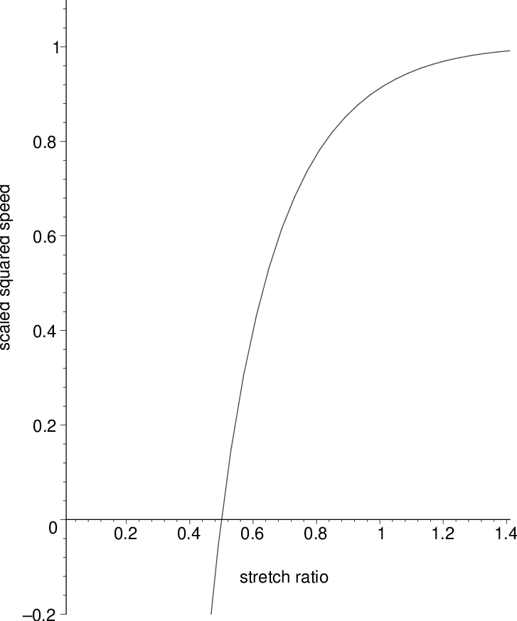
In Figure 1(b), the influence of the prestrain upon the speed of the surface wave is illustrated in the case of plane strain ($\lambda_{3}=1$). On the abscissa, $\lambda_{1}$ is increased from a compressive value ($\lambda_{1}<1$) to a tensile value ($\lambda_{1}>1$). The coordinate on the ordinate is the squared surface wave speed, scaled with respect to the transverse bulk wave speed, that is $\rho v^{2}/(\mu\lambda_{1}^{2})$. At $\lambda_{1}=1$, the half-space is isotropic ($\lambda_{1}=\lambda_{2}=\lambda_{3}=1$) because of (8) and the scaled squared speed is equal to 0.9126, the value found by Lord Rayleigh [11] in the incompressible linear isotropic case. Under an increasing compressive load ($P_{1}>0$, $\lambda_{1}<1$), the surface wave speed decreases until the critical stretch of $(\lambda_{1}$)${}_{\text{cr}}=0.5$ (see §3.3). Conversely, under a tensile load ($P_{1}<0$, $\lambda_{1}>1$), the surface wave speed increases, with the speed of the transverse bulk wave as an upper bound.

For Bell’s empirical model materials [6], the strain energy function $\Sigma_{\text{BEM}}$ is given by

where $\beta_{0}$ is a positive constant. The material response functions $\omega_{0}$ and $\omega_{2}$ and the quantities $b_{3}$ and $C$ provided by (4) and (12) are now

In that context, the bifurcation criterion (22) may be arranged as

which is the stability equation (7.10) of Beatty and Pan [12] for this problem; it is actually a cubic for $\lambda_{1}$ and $\lambda_{2}$. It delimits a curved surface in the stretch ratios space ($\lambda_{1},\lambda_{2},\lambda_{3}$), which cuts the constraint plane (8) into a part which is “unstable” (in the linearized theory) and a part which is always stable (in the linearized theory). This partition of the triangle of possible stretch ratios is visible on Figure 2(a). By extension from the plane strain case where $\lambda_{3}=1$ (treated below), we deduce that the visible part of the triangle is the stable one. For a clearer picture, Figure 2(b) (where the plane of the Figure coincides with the plane of the triangle) shows the intersection between the triangle and the bifurcation curve.

For the propagating surface wave, we consider only the case where the underlying deformation is a plane strain such that $\lambda_{3}=1$. Then the Bell constraint (8) reduces to $\lambda_{1}+\lambda_{2}=2$, and neither $\lambda_{1}$ nor $\lambda_{2}$ may be greater than 2. Then the secular equation (24) reduces to:

As noted in the general case, $f(0)<0$. On the other hand, $f(1)=2(3\lambda_{1}-2)/\lambda_{1}^{2}$, and so, because $f$ is a monotone increasing function for $\eta>0$, there exists a root to the secular equation (32) in the interval $[0,1]$ if and only if: $3\lambda_{1}-2>0$; moreover, the root is unique.

The stability of a deformed half-space made of incompressible rubber was first studied by Biot. He used the neo-Hookean model but noted [2, p.165] that the results were also valid for the Mooney-Rivlin model (Flavin [13] solved explicitly this latter case.) Biot obtained the bifurcation criterion, showed that it was universal relative to both classes of materials, and computed the value of the critical stretch ($\lambda_{1}$)${}_{\text{cr}}$ at which the rubber half-space becomes “unstable” under compressive loads, first in the case of plane strain $\lambda_{3}=1$, then in the case of the biaxial strain $\lambda_{2}=\lambda_{3}$. Also, Green and Zerna [14, p.137] found the critical stretch for the biaxial prestrain $\lambda_{1}=\lambda_{3}$. In each case a cubic must be solved in order to evaluate the critical stretch. In the case of a general triaxial prestrain, the bifurcation criterion is as follows:

We now show that for Bell’s empirical models and for simple hyperelastic Bell materials, the critical stretch can be found explicitly.

First we let the half-space made of Bell-constrained material be deformed in such a way that there is no extension in the $x_{3}$-direction ($\lambda_{3}=1$). According to (9)_2,3, this deformation is possible when the loads $P_{1}=2(1-\lambda_{1})[\lambda_{1}\omega_{2}-\omega_{0}/(2-\lambda_{1})]$ and $P_{3}=(1-\lambda_{1})[\omega_{2}-\omega_{0}/(2-\lambda_{1})]$ are applied at infinity. Then $\lambda_{2}=2-\lambda_{1}$ by (8). For Bell’s empirical model and for simple hyperelastic Bell materials, the bifurcation criterion (27) reduces respectively to

Then we let the half-space made of Bell-constrained material expand freely in the $x_{3}$-direction, so that $P_{3}=0$. Then we have $\lambda_{2}=\lambda_{3}=(3-\lambda_{1})/2$ by (9)₃ and (8), and the load $P_{1}=(3/2)(1-\lambda_{1})[\lambda_{1}\omega_{2}-2\omega_{0}/(3-\lambda_{1})]$ must be applied at infinity to maintain the deformation. For Bell’s empirical model and for simple hyperelastic Bell materials, the bifurcation criterion (27) reduces respectively to

Finally we consider that the Bell material is subject to a biaxial prestrain such that $\lambda_{1}=\lambda_{3}$. Then $\lambda_{2}=3-2\lambda_{1}$ and $P_{1}=P_{3}=3(1-\lambda_{1})[\lambda_{1}\omega_{2}-\omega_{0}/(3-2\lambda_{1})]$. For Bell’s empirical model and for simple hyperelastic Bell materials, the bifurcation criterion (27) reduces respectively to

In Table 1, the numerical values for the critical stretches are given for the classes of Bell’s empirical model (2nd column), of neo-Hookean and Mooney-Rivlin incompressible materials [2, 14] (3rd column), and of simple hyperelastic Bell materials (4th column), in the cases of plane strain (3rd row) and of biaxial strain (2nd and 4th rows). It appears that rubber can be compressed more than Bell’s empirical model but less than simple hyperelastic Bell materials, before it loses its near-the-surface stability (in the linearized theory).

Table 1: Critical stretch ratios $(\lambda_{1})_{\text{cr}}$ for surface instability Bell empirical rubber simple Bell $\lambda_{1}=\lambda_{3}$ 0.706 0.666 0.600 $\lambda_{3}=1$ 0.667 0.544 0.500 $\lambda_{2}=\lambda_{3}$ 0.545 0.444 0.429

The strain energy functions for the Mooney-Rivlin model and for the simple hyperelastic Bell material depend both upon two distinct material constants:

respectively, where $\mathcal{D}_{1}$, $\mathcal{D}_{2}$ are constants and $I_{1}$, $I_{2}$ are the first two invariants of the left Cauchy-Green tensor $\mathbf{B}=\mathbf{V}^{2}$. The fact that their bifurcation criteria are ‘relative-universal’ [15] to each class might come as a surprising result, but is easily understood once the strain energy functions are written in terms of the principal stretches of the deformation [9] as $\Sigma_{\text{MR}}(I_{1},I_{2})\equiv W_{\text{MR}}(\lambda_{1},\lambda_{2},\lambda_{3})$ and $\Sigma_{\text{SHB}}(i_{2},i_{3})\equiv W_{\text{SHB}}(\lambda_{1},\lambda_{2},\lambda_{3})$, where

Indeed, the bifurcation criterion for a general incompressible hyperelastic half-space may be written in terms of the first and second derivatives of its strain energy function $W$ with respect to $\lambda_{i}$ ($i=1,2$) as [9],

When $W$ is specialized to the Mooney-Rivlin form (38)₁, it yields the relative-universal bifurcation criterion (33). In fact, many subclasses of incompressible materials have a relative-universal bifurcation criterion. For instance, any incompressible material with the following strain energy function,

(where $n=1,2,3,$…) has the following relative-universal bifurcation criterion:

In particular, the bifurcation criterion (27), which happens to coincide with (41) when $n=1$, is also valid for incompressible Varga materials ($n=1$ in (40)).

Turning back to Bell-constrained materials, we note that it is a simple matter to write the quantities $b_{3}$ and $C$ in (12) in terms of the derivatives of $W(\lambda_{1},\lambda_{2},\lambda_{3})$. We find that

so that the bifurcation criterion (22) for Bell materials is rewritten as

When $W$ is specialized to the simple hyperelastic Bell model (38)₂, it yields the relative-universal bifurcation criterion (27). Similarly, when $W$ is specialized to the strain energy function of the Bell empirical model (29), written as

it yields the bifurcation criterion (31).

References

- [1] M.A. Biot, Acoustics, Elasticity, and Thermodynamics of Porous Media: Twenty-One Papers by M.A. Biot. Ed: I. Tolstoy (Acoustical Society of America, New-York, 1991).
- [2] —–, Mechanics of Incremental Deformations, John Wiley, New-York (1965).
- [3] M.F. Beatty and M.A. Hayes, J. Elasticity 29, 1–84 (1992).
- [4] M. Destrade, Int. J. Nonlinear Mech. 38, 809–814 (2002).
- [5] M. Romeo, J. Acoust. Soc. Am. 110, 59–67 (2001).
- [6] J.F. Bell, Int. J. Plasticity 1, 3–27 (1985).
- [7] M.F. Beatty and M.A. Hayes, Q. Jl. Mech. Appl. Math. 45, 663–709 (1992).
- [8] —– and —–, Z.A.M.P. 46, 356–371 (1995).
- [9] M.A. Dowaikh and R.W. Ogden, IMA J. Appl. Math. 44, 261–284 (1990).
- [10] M. Destrade, Maths. Mech. Solids (submitted).
- [11] Lord Rayleigh, Proc. R. Soc. London A17, 4–11 (1885).
- [12] M.F. Beatty and F.X. Pan, Int. J. Non-Linear Mech. 33, 867–906 (1998).
- [13] J.N. Flavin, Q. Jl. Mech. Appl. Math. 16, 441–449 (1963).
- [14] A.E. Green and W. Zerna, Theoretical Elasticity, Dover, New-York (1992).
- [15] G. Saccomandi, In: Nonlinear Elasticity: Theory and Applications. Eds: Y.B. Fu and R.W. Ogden, 97–134 (Cambridge University Press, London, 2001).
- [16] P. Chadwick and D.A. Jarvis, Proc. R. Soc. London A366, 517–536 (1979).
- [17] A.N. Guz, Fundamentals of the Three-Dimensional Theory of Stability of Deformable Bodies, Springer-Verlag, Berlin (1999).
- [18] M.A. Biot, H. Odé, and W.L. Roever, Geol. Soc. America Bull. 72, 1621–1632 (1961).
- [19] Y.B. Fu, Proc. Roy. Soc. London A443, 59–82 (1993).
- [20] Y.B. Fu and G.A. Rogerson, —– A446, 233–254 (1994).
- [21] M.F. Beatty, In: Nonlinear Elasticity: Theory and Applications. Eds: Y.B. Fu and R.W. Ogden, 58–96 (Cambridge University Press, London, 2001).
- [22] H.S. Sellers and A.S. Douglas, Int. J. Plast. 6, 329–351 (1990).
- [23] D.J. Steigmann, Meccanica (to appear).
- [24] E. Pucci and G. Saccomandi, Math. Mech. Solids 1, 207–217 (1996).
- [25] M.M. Carroll, Acta Mech. 3, 167–181 (1967).
- [26] G. Saccomandi, In: Topics in Finite Elasticity, CISM Courses and Lectures No. 424. Eds: M. Hayes and G. Saccomandi, 95–130 (Springer-Verlag, Vienna, 2001).
List of Figures and Tables
Figure 1: Near-the-surface stability for ‘simple hyperelastic Bell’ materials.
Figure 1(a): Region of stability.
Legend on graduated axes: “”, “”, and “”.
Figure 1(b): Surface wave speed.
Legend on graduated horizontal axis: “stretch ratio”.
Legend on graduated vertical axis: “scaled squared speed”.
Figure 2: Near-the-surface stability for ‘Bell empirical model’ materials.
Figure 2(a): Region of stability.
Figure 2(b): Bifurcation curve in triangle.