跳到论文正文
W Papers独立论文阅读器 arXiv:1304.7834 论文正文 计算阅读时间 · 0%
引用这篇论文根据当前论文元数据生成,正式投稿前建议核对。


License: arXiv.org perpetual non-exclusive license
arXiv:1304.7834v1 [physics.bio-ph] 30 Apr 2013

Noise-assisted quantum electron transfer in photosynthetic complexes

Preprint: LA-UR-13-23059
Alexander I. Nesterov Email: nesterov@cencar.udg.mx Affiliation: Departamento de Física, CUCEI, Universidad de Guadalajara, Av. Revolución 1500, Guadalajara, CP 44420, Jalisco, México    Gennady P. Berman Email: gpb@lanl.gov Affiliation: Theoretical Division, Los Alamos National Laboratory, Los Alamos, NM 87544, USA    José Manuel Sánchez Martínez Email: jmsm.manuel@gmail.com Affiliation: Departamento de Física, CUCEI, Universidad de Guadalajara, Av. Revolución 1500, Guadalajara, CP 44420, Jalisco, México    Richard T. Sayre Email:  rsayre@newmexicoconsortium.org Affiliation: Los Alamos National Laboratory and New Mexico Consortium, 4200 W James Rd, Los Alamos, NM, 87544, USA
August 24, 2026
Abstract

Electron transfer (ET) between primary electron donors and acceptors is modeled in the photosystem II reaction center (RC). Our model includes (i) two discrete energy levels associated with donor and acceptor, interacting through a dipole-type matrix element and (ii) two continuum manifolds of electron energy levels (“sinks”), which interact directly with the donor and acceptor. Namely, two discrete energy levels of the donor and acceptor are embedded in their independent sinks through the corresponding interaction matrix elements. We also introduce classical (external) noise which acts simultaneously on the donor and acceptor (collective interaction). We derive a closed system of integro-differential equations which describes the non-Markovian quantum dynamics of the ET. A region of parameters is found in which the ET dynamics can be simplified, and described by coupled ordinary differential equations. Using these simplified equations, both sharp and flat redox potentials are analyzed. We analytically and numerically obtain the characteristic parameters that optimize the ET rates and efficiency in this system.

Keywords: 
non-Hermitian Hamiltonian, reaction center, electron transfer, noise, sink
pacs
87.15.ht, 05.60.Gg, 82.39.Jn

I Introduction

In photosynthetic complexes of plants, eukaryotic algae and cyanobacteria, quanta of light excite chlorophyll dipoles in the antennas of the light harvesting complexes. These local energy excitations are then transferred to the reaction centers (RCs) of photosystem I (PSI) and photosystem II (PSII), where the charge separation occurs. During charge separation an electron jumps from the donor to the acceptor and both donor and acceptor become charged. These electron jumps continue through out the whole chain of the redox potential. The characteristic time-scales of the electron dynamics vary from a few picoseconds to milliseconds. The primary charge separation occurs on a very short time-scale, of a few picoseconds [1, 2, 3, 4, 5]. Because this time-scale is so short, even the room-temperature fluctuations of the protein environment do not destroy the quantum coherent effects, which were recently discovered in these complexes [5, 6, 7, 8, 9, 10, 11, 12, 13].

Generally, to describe the motion of an electron between the donor and acceptor, different approaches can be used [15, 5, 14, 16, 17, 18, 19, 20, 21]. The leading approach is based on the well-known Markus theory, which takes into account both the strength of donor-acceptor interaction, distance and the dynamics of the protein environment [14]. In this way, the election transfer (ET) rate and the efficiency of the ET can be calculated [15]. At the same time, many efforts have been devoted to various modifications of the Markus theory. One of them is related to taking into account the sinks which represent the continuum electron energy reservoirs analogous to the HOMO and LUMO orbitals in the chemical systems [12, 13, 22] (see also references therein). These continuum manifolds are similar to those described by the Weisskopf-Wigner model [23, 24]. These sinks serve as additions to the thermal reservoirs in ET. The principal difference between the protein (vibrational) and sink reservoirs is that the former behave as the bosonic (electromagnetic) environments while the later provide additional electron quasi-degenerate states. These sinks increase the entropy for an electron escaping into the sinks. As a result, the sinks modify the form of the Gibbs equilibrium distribution. Indeed, even in the case of a flat redox potential one can expect the acceptor to be populated with high enough efficiency.

In this paper, we consider ET in a model which consists of two discrete energy states, donor and acceptor. A dipole-type matrix element of a direct donor-acceptor interaction is included. The donor and acceptor interact directly with two independent sinks which are represented by two quasi-degenerate (continuum) manifolds of the electron energy levels. In addition, classical (external) noise interacts with the donor and the acceptor. By taking into account these effects, we describe the ET dynamics in different parameter region. We obtain the conditions when the system of integro-differential equations, which describes generally the non-Markovian electron dynamics, can be reduced to much simpler system of ordinary differential equations. We obtain analytically and numerically the ET for both sharp and flat redox potentials, and for different amplitudes of noise. The advantage of our approach is that it is a rigorous one, so all approximations are controlled and justified. The simultaneous contributions of the sinks and noise are analyzed, allowing us to derive optimal ET rates for various regions of parameters.

Our paper is organized as follows. In Section II, we describe our simplified model with a single sink interacting only with the acceptor level, and present an analytic solution for the ET, in the absence of noise. In Section III, we analyze analytically and numerically the simultaneous influence of the single acceptor sink and noise. We derive a closed system of integro-differential equations which describe the ET. We also find the region of parameters for which a system of ordinary differential equations can be applied. In Section IV, we analyze analytically and numerically the simultaneous influence of two sinks and noise. In Section V, we discuss the obtained results. In the Appendices some useful formulae are presented.

II Model description

Our model consists of two protein cofactors in the RC (donor and acceptor) each with a discrete energy level. In this Section, we consider, for simplicity, only a single sink which interacts with the acceptor level (the acceptor is also embedded in a sink). The sink can be considered either as an additional, third cofactor, or as a part of the acceptor. (See Fig. 1.) The first site, denoted by |d⟩|d\rangle, is the electron donor, with the energy level, EdE_{d}. The second site, |a⟩|a\rangle, is the electron acceptor, with energy level, EaE_{a}. We model the sink by a large number of discrete and nearly degenerate energy levels, Na≫1N_{a}\gg 1 (Fig. 1). Then, the transition to the high density of states (in the continuum limit) is done for the sink.

Refer to caption
Figure 1: Schematic of our model consisting of donor and acceptor discrete energy levels, with the acceptor coupled to a sink reservoir with a nearly continuous spectrum.

Note that in some situations, the sinks can be considered as approximations to HOMO and LUMO orbitals with finite densities of states.

The Hamiltonian of this system can be written as

Ht=Ed​|d⟩​⟨d|+Ea|a⟩​⟨a|+V2​(|d⟩​⟨a|+|a⟩​⟨d|)\displaystyle H_{t}=E_{d}|d\rangle\langle d|+E_{a}|a\rangle\langle a|+\frac{V}{2}(|d\rangle\langle a|+|a\rangle\langle d|)
+∑i=1NEi|i⟩⟨i|+∑i=1Na(Va​i|a⟩⟨i|+Vi​a|i⟩⟨a|),\displaystyle+\sum^{N}_{i=1}E_{i}|i\rangle\langle i|+\sum^{N_{a}}_{i=1}\big(V_{ai}|a\rangle\langle i|+V_{ia}|i\rangle\langle a|\big), (1)

where EiE_{i} are energies of the sink levels, and Vd​a=V/2V_{da}=V/2. (See Fig. 1.)

Using the standard Feshbach projection method [24, 25, 26, 27, 28], one can show that the dynamics of the donor-acceptor (intrinsic) states can be described by the following Schrödinger equation with an effective non-Hermitian Hamiltonian, ℋ~=ℋ−i​𝒲\tilde{\mathcal{H}}={\mathcal{H}}-i\mathcal{W} (we set ℏ=1\hbar=1)[29]:

i​∂ψ⁡(t)∂t=ℋ~​ψ​(t),\displaystyle i\frac{\partial\psi(t)}{\partial t}=\tilde{\mathcal{H}}\psi(t), (2)

where

ℋ=εd​|d⟩​⟨d|+εa|a⟩​⟨a|+V2​(|d⟩​⟨a|+|a⟩​⟨d|)\displaystyle{\mathcal{H}}=\varepsilon_{d}|d\rangle\langle d|+\varepsilon_{a}|a\rangle\langle a|+\frac{V}{2}(|d\rangle\langle a|+|a\rangle\langle d|) (3)

is the dressed donor-acceptor Hamiltonian, and 𝒲=(Γa/2)​|a⟩​⟨a|\mathcal{W}=({\Gamma_{a}}/{2})|a\rangle\langle a|. Here Γa\Gamma_{a} is the rate describing the tunneling from the acceptor to the sink. (See Appendix A for details.)

Equivalently, the dynamics of this system can be described by the Liouville equation,

i​ρ˙=[ℋ,ρ]−i⁡{𝒲,ρ},\displaystyle i\dot{\rho}=[\mathcal{H},\rho]-i\{\mathcal{W},\rho\}, (4)

where ρ\rho is the density matrix projected on the intrinsic states, and {𝒲,ρ}=𝒲​ρ+ρ​𝒲\{\mathcal{W},\rho\}=\mathcal{W}\rho+\rho\mathcal{W}.

The solution of the eigenvalue problem for the effective non-Hermitian Hamiltonian, ℋ~\tilde{\mathcal{H}}, yields two complex eigenvalues: E~1,2=λ~0/2±Ω/2\tilde{E}_{1,2}=\tilde{\lambda}_{0}/2\pm\Omega/2, where λ~0=εd+εa−i​Γ\tilde{\lambda}_{0}=\varepsilon_{d}+\varepsilon_{a}-i\Gamma and Ω=V2+(ε+i​Γ)2\Omega=\sqrt{V^{2}+(\varepsilon+i\Gamma)^{2}}. Here we denote ε=εd−εa\varepsilon=\varepsilon_{d}-\varepsilon_{a} and Γ=Γa/2\Gamma=\Gamma_{a}/2. The eigenvalues coalescence in the so-called exceptional point (EP) defined by the equation, Ω⁡(V,ε,Γ)=0\Omega(V,\varepsilon,\Gamma)=0. Since Ω\Omega is a complex function of its parameters, we obtain two real equations: ℜ⁡Ω=0\Re\Omega=0 and ℑ⁡Ω=0\Im\Omega=0. One can show that these equations are equivalent to ε=0\varepsilon=0 and V=ΓV=\Gamma.

Note that, in contrast to the case of an Hermitian Hamiltonian, where the degeneracy is referred to as a “conical intersection” (known also as a “diabolic point” [30]), the coalescence of eigenvalues results in different eigenvectors. At the EP, the eigenvectors merge, forming a Jordan block. (See the review [31], and references therein.)

Choice of parameters. This model involves various parameters, whose values are only partially known. Our choice of parameters is based on the data taken for the ET through the active pathway in the quinone-type of the Photosystem II RC [32]. (Note that the values of parameters in energy units can be obtained by multiplying our values by ℏ≈6.58×10⁻¹³​meVs\hbar\approx 6.58\times 10^{-13}\rm meVs. For example, ε=60​ps−1≈40​m​e​V\varepsilon=60\;\rm ps^{-1}\approx 40\rm meV.)

II.1 Tunneling to the sink

In this section we discuss the ET to the sink. (For details see [29].) We assume that initially the electron occupies the upper level (donor), ρ11​(0)=1\rho_{11}(0)=1 and ρ22​(0)=0\rho_{22}(0)=0. With these initial conditions, the solution of the Liouville equation (87) for the diagonal component of the density matrix is:

ρ11​(t)=\displaystyle\rho_{11}(t)= e−Γ​t​|(cos⁡Ω​t2−i​cos⁡θ​sin⁡Ω​t2)|2,\displaystyle{e^{-\Gamma t}}\bigg|\Big(\cos\frac{\Omega t}{2}-i\cos\theta\sin\frac{\Omega t}{2}\Big)\bigg|^{2}, (5)
ρ22​(t)=\displaystyle\rho_{22}(t)= e−Γ​t​|sin⁡θ​sin⁡Ω​t2|2,\displaystyle{e^{-\Gamma t}}\bigg|\sin\theta\sin\frac{\Omega t}{2}\bigg|^{2}, (6)

where Ω=V2+(ε+i​Γ)2\Omega=\sqrt{V^{2}+(\varepsilon+i\Gamma)^{2}} is the complex Rabi frequency, cos⁡θ=(ε+i​Γ)/Ω\cos\theta=(\varepsilon+i\Gamma)/\Omega, and sin⁡θ=V/Ω\sin\theta=V/\Omega.

Setting Ω=Ω1+i​Ω2=p+i​q\Omega=\Omega_{1}+i\Omega_{2}=\sqrt{p+iq}, where p=V2+ε2−Γ2p=V^{2}+\varepsilon^{2}-\Gamma^{2} and q=2​ε​Γq=2\varepsilon\Gamma, we obtain

Ω1=\displaystyle\Omega_{1}= ±12​p+p2+q2,\displaystyle\pm\frac{1}{\sqrt{2}}\sqrt{p+\sqrt{p^{2}+q^{2}}}, (7)
Ω2=\displaystyle\Omega_{2}= ±12​−p+p2+q2.\displaystyle\pm\frac{1}{\sqrt{2}}\sqrt{-p+\sqrt{p^{2}+q^{2}}}. (8)

Using these results, we obtain for ρ22​(t)\rho_{22}(t) the simple analytical expression:

ρ22(t)=V2​e−Γ​t2​(Ω12+Ω22)(coshΩ2t−cosΩ1t).\displaystyle\rho_{22}(t)=\frac{V^{2}e^{-\Gamma t}}{2(\Omega^{2}_{1}+\Omega^{2}_{2})}\big(\cosh{\Omega_{2}t}-\cos{\Omega_{1}t}\big). (9)

We define the ET efficiency of tunneling to the sink as

η⁡(t)=1−Tr⁡(ρ⁡(t))=∫0tTr⁡{𝒲,ρ⁡(τ)}​𝑑τ.\displaystyle\eta(t)=1-{\rm Tr}(\rho(t))=\int_{0}^{t}{\rm Tr}\{\mathcal{W},\rho(\tau)\}d\tau. (10)

This can be recast as the integrated probability of trapping the electron in the sink [10, 33],

η⁡(t)=2​Γ​∫0tρ22​(τ)​𝑑τ.\displaystyle\eta(t)=2\Gamma\int_{0}^{t}\rho_{22}(\tau)d\tau. (11)

Inserting ρ22​(t)\rho_{22}(t) into (11) and performing the integration, we find that the ET efficiency is given by

η⁡(t)=\displaystyle\eta(t)= 1−e−Γ​tΓ⁡(Ω12+Ω22)((Γ2+Ω12)(ΓcoshΩ2t+Ω2sinhΩ2t)\displaystyle 1-\frac{e^{-\Gamma t}}{\Gamma(\Omega^{2}_{1}+\Omega^{2}_{2})}\big((\Gamma^{2}+\Omega_{1}^{2})(\Gamma\cosh{\Omega_{2}t}+\Omega_{2}\sinh{\Omega_{2}t})
−(Γ2−Ω22)(ΓcosΩ1t−Ω1sinΩ1t)).\displaystyle-(\Gamma^{2}-\Omega_{2}^{2})(\Gamma\cos{\Omega_{1}t}-\Omega_{1}\sin{\Omega_{1}t})\big). (12)

In [29] it was shown that, for the sharp redox potential, the ET efficiency is rather slow function of time. For instance, for ε=60​ps−1\varepsilon=60\rm\,ps^{-1} and 10​ps<V<40​ps−110\rm\,ps<V<40\rm\,ps^{-1}, the ET efficiency approaches a value close to 1 for relatively large times, t≳150t\gtrsim 150 ps. However, the situation is changes drastically for the flat redox potential. For example, for ε=0\varepsilon=0, we obtain

Ω2=0,Ω12=V2−Γ2,V>Γ,Ω1=0,Ω2=0,V=ΓΩ1=0,Ω22=Γ2−V2,Γ>V.\displaystyle\begin{array}[]{l l l}\Omega_{2}=0,&\Omega_{1}^{2}=V^{2}-\Gamma^{2},&V>\Gamma,\\ \Omega_{1}=0,&\Omega_{2}=0,&V=\Gamma\\ \Omega_{1}=0,&\Omega_{2}^{2}=\Gamma^{2}-V^{2},&\Gamma>V.\end{array}

Using these relations, we find that at the exceptional point the ET efficiency behaves as

η⁡(t)=1−e−Γ​t.\displaystyle\eta(t)=1-e^{-\Gamma t}. (16)

For V≪ΓV\ll\Gamma ( V≫ΓV\gg\Gamma) the asymptotic behavior of η⁡(t)\eta(t) is

η⁡(t)∼{1−e−Γ​t,V≫Γ,1−e−V2t/2Γ,V≪Γ.\displaystyle\eta(t)\sim\left\{\begin{array}[]{ll}1-e^{-\Gamma t},&V\gg\Gamma,\\ 1-\displaystyle e^{-V^{2}t/2\Gamma},&V\ll\Gamma.\end{array}\right.

Comparing the obtained results with (12), we conclude that the highest ET rate is obtained for the flat redox potential at ε=0\varepsilon=0, and V≥ΓV\geq\Gamma. This result can be interpreted by using a model of a single spin dynamics in an effective magnetic field. The above parameters are defined so that the effective magnetic field is oriented in the positive xx-direction, and VV corresponds to the Rabi frequency–the frequency of rotation of the spin around the xx-axis. Then, the above chosen conditions provide a rapid transition from the donor to the acceptor, with subsequent tunneling from the acceptor to the sink. The results of numerical simulations of the ET efficiency are presented in Fig.  2. One can see that, when ε=0\varepsilon=0 and V≥ΓV\geq\Gamma, the ET efficiency can approach a value close to 1 for short enough times, ∼2\sim 2 ps.

Refer to caption
Refer to caption
Figure 2: (Color online) Time dependence (in ps) of the sites population, ρ11​(t)\rho_{11}(t) and ρ22​(t)\rho_{22}(t), (top) and ET efficiency (bottom) (Γ=5​ps−1\Gamma=5\,\rm ps^{-1}). Solid and dashed lines correspond to, ρ11​(t)\rho_{11}(t) and ρ22​(t)\rho_{22}(t), respectively. Blue line: V=10​ps−1,ε=0V=10\,\rm ps^{-1},\,\varepsilon=0; red line (EP): V=Γ=5​ps−1,ε=0V=\Gamma=5\,\rm ps^{-1},\,\varepsilon=0; green line: V=10​ps−1,ε=10​ps−1V=10\,\rm ps^{-1},\,\varepsilon=10\,\rm ps^{-1}; black line: V=5​ps−1,ε=20​ps−1V=5\,\rm ps^{-1},\,\varepsilon=20\,\rm ps^{-1}.

III Noise-assisted electron transfer to the sink

In the presence of classical noise, the quantum dynamics of the ET can be described by the following effective non-Hermitian Hamiltonian (for details see Appendix A):

ℋ~=\displaystyle\tilde{\mathcal{H}}= ∑nεn​|n⟩​⟨n|+∑m,nλm​n​(t)​|m⟩​⟨n|\displaystyle\sum_{n}\varepsilon_{n}|n\rangle\langle n|+\sum_{m,n}\lambda_{mn}(t)|m\rangle\langle n|
+V2∑m≠n|m⟩⟨n|−iΓ22|2⟩⟨2|,m,n=1,2,\displaystyle+\frac{V}{2}\sum_{m\neq n}|m\rangle\langle n|-i\frac{\Gamma_{2}}{2}|2\rangle\langle 2|,\quad m,n=1,2, (19)

where λm​n​(t)\lambda_{mn}(t) describes the noise. We denote by |1⟩|1\rangle and |2⟩|2\rangle the donor and acceptor states in the site representation, respectively. The diagonal matrix elements of noise, λn​n\lambda_{nn}, are responsible for decoherence, and the off-diagonal matrix elements, λm​n\lambda_{mn} (m≠nm\neq n), lead to the relaxation processes. In what follows, we use a spin-fluctuator model of noise, modeling the noise by an ensemble of fluctuators [34, 35, 36].

The evolution of the average diagonal components of the density matrix is described by the following system of integro-differential equations (see Appendix B):

dd​t​⟨ρ11​(t)⟩=\displaystyle\frac{d}{dt}{\langle{\rho}}_{11}(t)\rangle= −∫0tK(t,t′)(⟨ρ11(t′)⟩−⟨ρ22(t′)⟩)dt′,\displaystyle-\int_{0}^{t}{K}(t,t^{\prime})\big(\big\langle{\rho}_{11}(t^{\prime})\big\rangle-\big\langle{\rho}_{22}(t^{\prime})\big\rangle\big)dt^{\prime}, (20)
dd​t​⟨ρ22​(t)⟩=\displaystyle\frac{d}{dt}{\langle{\rho}}_{22}(t)\rangle= ∫0tK⁡(t,t′)​(⟨ρ11​(t′)⟩−⟨ρ22​(t′)⟩)​d​t′\displaystyle\int_{0}^{t}{K}(t,t^{\prime})\big(\big\langle{\rho}_{11}(t^{\prime})\big\rangle-\big\langle{\rho}_{22}(t^{\prime})\big\rangle\big)dt^{\prime}
−2​Γ​⟨ρ22​(t)⟩,\displaystyle-2\Gamma\langle{\rho}_{22}(t)\rangle, (21)

where the average ⟨⟩\langle\;\rangle is taken over the random process describing noise, and the kernel, K⁡(t,t′)K(t,t^{\prime}), is given by

K⁡(t,t′)=e−Γ⁡(t−t′)​(⟨V~21​(t)​V~12​(t′)⟩+⟨V~21​(t′)​V~12​(t)⟩).\displaystyle K(t,t^{\prime})=e^{-\Gamma(t-t^{\prime})}\big(\big\langle{\tilde{V}}_{21}(t){\tilde{V}}_{12}(t^{\prime})\big\rangle+\big\langle{\tilde{V}}_{21}(t^{\prime}){\tilde{V}}_{12}(t)\big\rangle\big). (22)

In the rest of this paper, we restrict ourselves to considering only the diagonal noise effects, assuming that the noisy environment is the same for both the donor and the acceptor sites (collective noise). Then, one can write λ1​(t)=g1​ξ​(t)\lambda_{1}(t)=g_{1}\xi(t) and λ2​(t)=g2​ξ​(t)\lambda_{2}(t)=g_{2}\xi(t), where g1,2g_{1,2} are the interaction constants, and ξ⁡(t)\xi(t) is a random variable describing a stationary noise with the correlation function, χ⁡(t−t′)=⟨ξ⁡(t)​ξ​(t′)⟩,\chi(t-t^{\prime})=\langle\xi(t)\xi(t^{\prime})\rangle, given by [36]

χ⁡(τ)=σ2​A​(E1​(2​γm​τ)−E1​(2​γc​τ)),τ=|t−t′|.\displaystyle\chi(\tau)=\sigma^{2}A\Big(E_{1}(2\gamma_{m}\tau)-E_{1}(2\gamma_{c}\tau)\Big),\quad\tau=|t-t^{\prime}|. (23)

Here En​(z)E_{n}(z) denotes the Exponential integral [37], A=1/ln⁡(γc/γm)A=1/\ln(\gamma_{c}/\gamma_{m}), σ2=χ⁡(0)\sigma^{2}=\chi(0) and γm\gamma_{m} and γc\gamma_{c} (γm≪γc\gamma_{m}\ll\gamma_{c}) indicate the boundaries of the switching rates in the ensemble of random fluctuators. The correlation function includes, besides the amplitude, σ\sigma, two fitting parameters: γm\gamma_{m} and γc\gamma_{c}. Taking into account available theoretical and experimental data [38, 39, 40], we have chosen for our numerical simulations the parameters γm\gamma_{m} and γc\gamma_{c} as follows: 2​γm=10−4​ps−12\gamma_{m}=10^{-4}\rm ps^{-1}, 2​γc=1​ps−12\gamma_{c}=1\rm ps^{-1}.

Using the Gaussian approximation, we obtain the following expression for the kernel (see Appendix B):

K⁡(t−t′)=V22​cos⁡(ε⁡(t−t′))​exp⁡(−Γ⁡(t−t′)−⟨κ2​(t−t′)⟩2),\displaystyle K(t-t^{\prime})=\frac{V^{2}}{2}\cos(\varepsilon(t-t^{\prime}))\exp\bigg(-\Gamma(t-t^{\prime})-\frac{\langle\kappa^{2}(t-t^{\prime})\rangle}{2}\bigg), (24)

where

⟨κ2​(t−t′)⟩=2​D2​∫0t−t′d​τ′​∫0τ′d​τ′′​χ​(τ′−τ′′),\displaystyle\langle\kappa^{2}(t-t^{\prime})\rangle=2D^{2}\int^{t-t^{\prime}}_{0}d\tau^{\prime}\int_{0}^{\tau^{\prime}}d\tau^{\prime\prime}\chi(\tau^{\prime}-\tau^{\prime\prime}), (25)

and we denote D=|g1−g2|D=|g_{1}-g_{2}|. The result of integration with the correlation function (23) is given by [36]

⟨κ2​(τ)⟩=\displaystyle\langle\kappa^{2}(\tau)\rangle= D2​σ2​A​(E3​(2​γm​τ)4​γm2−E3​(2​γc​τ)4​γc2CLOSE\displaystyle D^{2}\sigma^{2}A\bigg(\frac{E_{3}(2\gamma_{m}\tau)}{4\gamma_{m}^{2}}-\frac{E_{3}(2\gamma_{c}\tau)}{4\gamma_{c}^{2}}
OPEN+τ4​γm2−τ4​γc2+14​γc2−14​γm2)\displaystyle+\frac{\tau}{4\gamma_{m}^{2}}-\frac{\tau}{4\gamma_{c}^{2}}+\frac{1}{4\gamma_{c}^{2}}-\frac{1}{4\gamma_{m}^{2}}\bigg) (26)

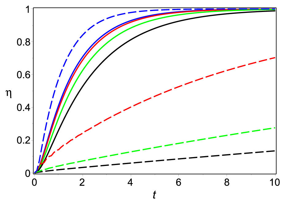
In Figs. 3 and 4 we present the results of numerical simulations for the tunneling rate, Γ=1​ps−1\Gamma=1\,\rm ps^{-1}, and different parameters, VV, ε\varepsilon, and the amplitude of noise, D​σD\sigma. As one can see from Fig.  3, a low level of the noise does not improve the ET efficiency rates. However, if the amplitude is sufficiently large, the noise significantly accelerates the ET to the sink (Fig.  4).

In [29] we show that for a sharp redox potential, noise can greatly improve the rate of ET to the sink. Our numerical results presented in Fig. 4, demonstrate that this is true for any redox potential, if the noise is strong enough.

Refer to caption
Figure 3: (Color online) Time dependence (ps) of the ET efficiency (V=Γ=1​ps−1V=\Gamma=1\,\rm ps^{-1}, D​σ=5​ps−1D\sigma=5\,\rm ps^{-1}). Blue line: ε=0\varepsilon=0 (EP), red line: ε=20​ps−1\varepsilon=20\,\rm ps^{-1}, green line: ε=40​ps−1\varepsilon=40\,\rm ps^{-1}, black line: ε=60​ps−1\varepsilon=60\,\rm ps^{-1}.
Refer to caption
Figure 4: (Color online) Time dependence (in ps) of the ET efficiency (V=10​ps−1V=10\,\rm ps^{-1}, Γ=1​ps−1\Gamma=1\,\rm ps^{-1} ). Solid lines correspond to η⁡(t)\eta(t) in the presence of noise with the amplitude D​σ=40​ps−1D\sigma=40\,\rm ps^{-1}. Blue line: ε=0\varepsilon=0, red line: ε=20​ps−1\varepsilon=20\,\rm ps^{-1}, green line: ε=40​ps−1\varepsilon=40\,\rm ps^{-1}, black line: ε=60​ps−1\varepsilon=60\,\rm ps^{-1}. Dashed lines correspond to η⁡(t)\eta(t), in the absence of noise.

In Fig. 5 we present the results of numerical simulations at the EP and in presence of noise for the tunneling rate Γ=5​ps−1\Gamma=5\,\rm ps^{-1} (ε=0,V=Γ=5​ps−1\varepsilon=0,V=\Gamma=5\,\rm ps^{-1}). As can be observed, at the exceptional point (EP) the noise decreases the rate of the ET. The behavior of the system in the vicinity of the EP is rather complicated, and the ET efficiency is sensitive to the choice of parameters (Fig. 6 ). For instance, for the flat redox potential with ε=0\varepsilon=0 and an amplitude of noise, D​σ=60​ps−1D\sigma=60\,\rm ps^{-1}, the ET efficiency approaches a value close to 1 for short enough time, ∼2\sim 2 ps.

Refer to caption
Figure 5: (Color online) Time dependence (in ps) of the ET efficiency at the EP in the presence of noise (ε=0,V=Γ=5​ps−1\varepsilon=0,V=\Gamma=5\,\rm ps^{-1}). Blue line: D​σ=0D\sigma=0, red line: D​σ=20​ps−1D\sigma=20\,\rm ps^{-1}, green line: D​σ=40​ps−1D\sigma=40\,\rm ps^{-1}, black line: D​σ=60​ps−1D\sigma=60\,\rm ps^{-1}.
Refer to caption
Figure 6: (Color online) Time dependence (in ps) of the ET efficiency in the vicinity of the EP in the presence of noise (ε=0,D​σ=60​ps−1,Γ=5​ps−1\varepsilon=0,D\sigma=60\,\rm ps^{-1},\Gamma=5\,\rm ps^{-1}). Blue line: V=2.5​ps−1V=2.5\,\rm ps^{-1}, red line: V=5​ps−1V=5\,\rm ps^{-1} (EP), green line: V=10​ps−1V=10\,\rm ps^{-1}, black line: V=20​ps−1V=20\,\rm ps^{-1}.

III.1 Electron transport approximated by differential equations

Under some conditions, the system of integro-differential equations,

dd​t​⟨ρ11​(t)⟩=\displaystyle\frac{d}{dt}{\langle{\rho}}_{11}(t)\rangle= −∫0tK(t,t′)(⟨ρ11(t′)⟩−⟨ρ22(t′)⟩)dt′,\displaystyle-\int_{0}^{t}{K}(t,t^{\prime})\big(\big\langle{\rho}_{11}(t^{\prime})\big\rangle-\big\langle{\rho}_{22}(t^{\prime})\big\rangle\big)dt^{\prime}, (27)
dd​t​⟨ρ22​(t)⟩=\displaystyle\frac{d}{dt}{\langle{\rho}}_{22}(t)\rangle= ∫0tK⁡(t,t′)​(⟨ρ11​(t′)⟩−⟨ρ22​(t′)⟩)​d​t′\displaystyle\int_{0}^{t}{K}(t,t^{\prime})\big(\big\langle{\rho}_{11}(t^{\prime})\big\rangle-\big\langle{\rho}_{22}(t^{\prime})\big\rangle\big)dt^{\prime}
−2​Γ​⟨ρ22​(t)⟩,\displaystyle-2\Gamma\langle{\rho}_{22}(t)\rangle, (28)

can be approximated by the following system of the ordinary differential equations:

dd​t​⟨ρ11​(t)⟩=\displaystyle\frac{d}{dt}{\langle{\rho}}_{11}(t)\rangle= −ℜ⁡(t)​(⟨ρ11​(t)⟩−⟨ρ22​(t)⟩),\displaystyle-{\mathfrak{R}}(t)\big(\big\langle{\rho}_{11}(t)\big\rangle-\big\langle{\rho}_{22}(t)\big\rangle\big), (29)
dd​t​⟨ρ22​(t)⟩=\displaystyle\frac{d}{dt}{\langle{\rho}}_{22}(t)\rangle= ℜ⁡(t)​(⟨ρ11​(t)⟩−⟨ρ22​(t)⟩)−2​Γ​⟨ρ22​(t)⟩,\displaystyle\,{\mathfrak{R}}(t)\big(\big\langle{\rho}_{11}(t)\big\rangle-\big\langle{\rho}_{22}(t)\big\rangle\big)-2\Gamma\langle{\rho}_{22}(t)\rangle, (30)

where ℜ⁡(t)=∫0tK⁡(τ)​𝑑τ{\mathfrak{R}}(t)=\int_{0}^{t}K(\tau)d\tau.

Below we obtain the conditions for which the exact system of integro-differential equations (27) - (28) can be approximated by Eqs. (29) - (30). In the first order of the series expansion, we can write

⟨ρ11​(t′)⟩≈⟨ρ11​(t)⟩−dd​t​⟨ρ11​(t)⟩​(t−t′),\displaystyle\langle{\rho}_{11}(t^{\prime})\rangle\approx\langle{\rho}_{11}(t)\rangle-\frac{d}{dt}{\langle{\rho}}_{11}(t)\rangle(t-t^{\prime}), (31)
⟨ρ22​(t′)⟩≈⟨ρ22​(t)⟩−dd​t​⟨ρ22​(t)⟩​(t−t′),\displaystyle\langle{\rho}_{22}(t^{\prime})\rangle\approx\langle{\rho}_{22}(t)\rangle-\frac{d}{dt}{\langle{\rho}}_{22}(t)\rangle(t-t^{\prime}), (32)

where, in the same order, the derivatives on the r.h.s. are taken from Eqs. (29), (30).

Using these results, after some transformations we find that Eqs. (27) - (28) become

dd​t​⟨ρ11​(t)⟩=\displaystyle\frac{d}{dt}{\langle{\rho}}_{11}(t)\rangle= −ℜ⁡(t)​(⟨ρ11​(t)⟩−⟨ρ22​(t)⟩)​(1−ℜ1​(t))\displaystyle-{\mathfrak{R}}(t)\big(\big\langle{\rho}_{11}(t)\big\rangle-\big\langle{\rho}_{22}(t)\big\rangle\big)(1-{\mathfrak{R}}_{1}(t))
+2​Γ​ℜ1​(t)​⟨ρ22​(t)⟩,\displaystyle+2\Gamma{\mathfrak{R}}_{1}(t)\langle{\rho}_{22}(t)\rangle, (33)
dd​t​⟨ρ22​(t)⟩=\displaystyle\frac{d}{dt}{\langle{\rho}}_{22}(t)\rangle= ℜ⁡(t)​(⟨ρ11​(t)⟩−⟨ρ22​(t)⟩)​(1−ℜ1​(t))\displaystyle\,{\mathfrak{R}}(t)\big(\big\langle{\rho}_{11}(t)\big\rangle-\big\langle{\rho}_{22}(t)\big\rangle\big)(1-{\mathfrak{R}}_{1}(t))
−2​Γ​⟨ρ22​(t)⟩​(1−ℜ1​(t)),\displaystyle-2\Gamma\langle{\rho}_{22}(t)\rangle(1-{\mathfrak{R}}_{1}(t)), (34)

where ℜ1​(t)=∫0tτ​K​(τ)​𝑑τ{\mathfrak{R}}_{1}(t)=\int_{0}^{t}\tau K(\tau)d\tau. From here it follows that the system of integro-differential equations (27) - (28) can be approximated by the system of the first order ordinary differential equations in the interval of time 0<t<∞0<t<\infty, if |∫0∞τ​K​(τ)​𝑑τ|≪1|\int_{0}^{\infty}\tau K(\tau)d\tau|\ll 1.

Assuming that the correlation function, χ⁡(t)\chi(t), is a rapidly decreasing function, as t→∞t\rightarrow\infty, we can approximate

exp(−D2∫0tdτ∫0τdsχ(τ−s))≈exp(−(D​σ​t)22).\displaystyle\exp\bigg(-D^{2}\int^{t}_{0}d\tau\int_{0}^{\tau}ds\,\chi(\tau-s)\bigg)\approx\exp\bigg(-\frac{(D\sigma t)^{2}}{2}\bigg). (35)
Refer to caption
Figure 7: (Color online) Dependence of δ\delta on ε\varepsilon and D​σD\sigma (Γ=1​ps−1\Gamma=1\,\rm ps^{-1}).

Performing the integration with the kernel

K⁡(τ)=V22​cos⁡(ε​τ)​exp⁡(−Γ​τ−(D​σ)22​τ2),\displaystyle K(\tau)=\frac{V^{2}}{2}\cos(\varepsilon\tau)\exp\bigg(-\Gamma\tau-\frac{(D\sigma)^{2}}{2}\tau^{2}\bigg), (36)

we obtain the following estimate:

|∫0∞K⁡(τ)​τ​𝑑τ|=|V2​δ2​D2​σ2|<V2​|δ|max2​D2​σ2≪1,\displaystyle\bigg|\int_{0}^{\infty}K(\tau)\tau d\tau\bigg|=\bigg|\frac{V^{2}\delta}{2D^{2}\sigma^{2}}\bigg|<\frac{V^{2}|\delta|_{\max}}{2D^{2}\sigma^{2}}\ll 1, (37)

where

δ=\displaystyle\delta= −1+π​q4​p​exp⁡(q24​p2)​erfc​(q2​p)\displaystyle-1+\frac{\sqrt{\pi}q}{4p}\exp\bigg(\frac{q^{2}}{4p^{2}}\bigg){\rm erfc}\bigg(\frac{q}{2p}\bigg)
+π​q¯4​p​exp⁡(q¯24​p2)​erfc​(q¯2​p),\displaystyle+\frac{\sqrt{\pi}\bar{q}}{4p}\exp\bigg(\frac{{\bar{q}}^{2}}{4p^{2}}\bigg){\rm erfc}\bigg(\frac{\bar{q}}{2p}\bigg), (38)

where p=D​σ/2p=D\sigma/\sqrt{2}, q=Γ+i​εq=\Gamma+i\varepsilon, q¯=Γ−i​ε\bar{q}=\Gamma-i\varepsilon, and erf​c​(z){\rm erf}c(z) denotes the complementary error function[37].

Using the properties of the erfc{\rm erfc} function, one can show that |δ|≤1|\delta|\leq 1 for any choice of parameters Γ,ε\Gamma,\varepsilon and the amplitude of noise, D​σD\sigma (Fig. 7). Consequently, the condition of validaty of the approximation (29) - (30) can be written as V≪D​σV\ll D\sigma. This rough estimate can be improved greatly for the high level of noise leading to V≤D​σV\leq D\sigma.

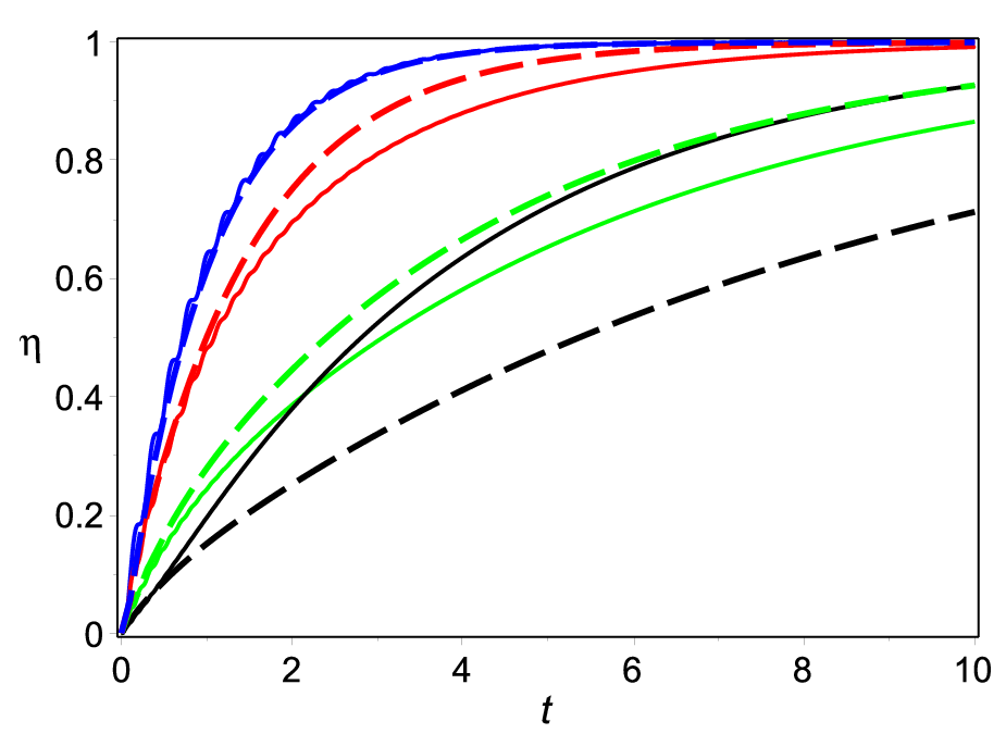
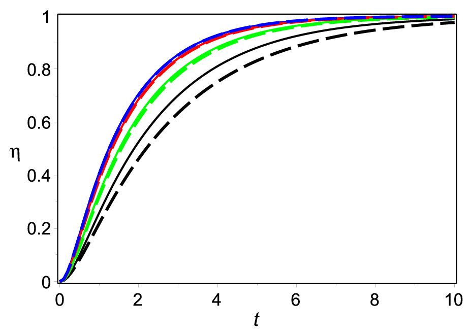
In Figs. 8, 9 we present the results of our numerical simulations for Γ=1​ps−1\Gamma=1\,\rm ps^{-1}. As one can see, for V≤D​σV\leq D\sigma there is good agreement between the solutions obtained from the system of integro-differential Eqs. (20)-(21) and the approximate system of differential Eqs. (29)-(30).
Refer to caption
Refer to caption
Figure 8: (Color online) Time dependence (in ps) of the ET efficiency, η⁡(t)\eta(t). The solutions of the system of integro-differential equations are presented by solid lines (Γ=1​ps−1\Gamma=1\,\rm ps^{-1}). Dashed lines correspond to the solutions of the approximate system of differential equations. Blue line: ε=0\varepsilon=0, red line: ε=20​ps−1\varepsilon=20\,\rm ps^{-1}, green line: ε=40​ps−1\varepsilon=40\,\rm ps^{-1}, black line: ε=60​ps−1\varepsilon=60\,\rm ps^{-1}. Top: V=30​ps−1V=30\,\rm ps^{-1}, D​σ=5​ps−1D\sigma=5\,\rm ps^{-1}. Bottom: V=10​ps−1V=10\,\rm ps^{-1}, D​σ=40​ps−1D\sigma=40\,\rm ps^{-1}.
Refer to caption
Figure 9: (Color online) Time dependence (in ps) of the ET efficiency. Solid lines correspond to η⁡(t)\eta(t) obtained from the system of integro-differential Eqs. (20)-(21) and dashed lines present the results for η⁡(t)\eta(t) obtained from the system of differential Eqs. (29)-(30). Blue line: ε=0\varepsilon=0, red line: ε=20​ps−1\varepsilon=20\,\rm ps^{-1}, green line: ε=40​ps−1\varepsilon=40\,\rm ps^{-1}, black line: ε=60​ps−1\varepsilon=60\,\rm ps^{-1} (Γ=1​ps−1\Gamma=1\,\rm ps^{-1}, V=D​σ=40​ps−1V=D\sigma=40\,\rm ps^{-1}). One can observe the excellent agreement between the solutions.

The advantage of using differential equations instead of integro-differential equations is (i) the ability to introduce effective rates and (ii) the ability to compare the results with the Markus theory. The computation of the asymptotic ET, ℜΓ=limt→∞ℜ⁡(t){\mathfrak{R}}_{\Gamma}=\lim_{t\rightarrow\infty}{\mathfrak{R}}(t), yields [29]

ℜΓ=\displaystyle{\mathfrak{R}}_{\Gamma}= V2​2​π8​D​σ​(exp⁡((Γ+i​ε)22​D2​σ2)​erfc​(Γ+i​ε2​D​σ)CLOSE\displaystyle\frac{V^{2}\sqrt{2\pi}}{8D\sigma}\Bigg(\exp\bigg(\frac{(\Gamma+i\varepsilon)^{2}}{2D^{2}\sigma^{2}}\bigg){\rm erfc}\bigg(\frac{\Gamma+i\varepsilon}{\sqrt{2}D\sigma}\bigg)
OPEN+exp⁡((Γ−i​ε)22​D2​σ2)​erfc​(Γ−i​ε2​D​σ)).\displaystyle+\exp\bigg(\frac{(\Gamma-i\varepsilon)^{2}}{2D^{2}\sigma^{2}}\bigg){\rm erfc}\bigg(\frac{\Gamma-i\varepsilon}{\sqrt{2}D\sigma}\bigg)\Bigg). (39)
Refer to caption
Figure 10: (Color online) Blue line describes the time dependence of the ET rate, ℜ⁡(t){\mathfrak{R}}(t). Red line corresponds to the asymptotic rate, ℜΓ{\mathfrak{R}}_{\Gamma}, given by Eq. (39). From top to bottom: ε=0, 20, 40, 60​ps−1\varepsilon=0,\,20,\,40,\,60\,\rm ps^{-1} (Γ=1​ps−1\Gamma=1\,\rm ps^{-1}, V=10​ps−1V=10\,\rm ps^{-1} and D​σ=40​ps−1D\sigma=40\,\rm ps^{-1}).
Refer to caption
Figure 11: (Color online) Dependence of the asymptotic rate, ℜΓ{\mathfrak{R}}_{\Gamma}, on ε\varepsilon and D​σD\sigma (V=10​ps−1V=10\,\rm ps^{-1}, Γ=1​ps−1\Gamma=1\,\rm ps^{-1}).

In Fig. 10, we compare the results of numerical calculations of the relaxation rate, ℜ⁡(t){\mathfrak{R}}(t) (blue line), with the asymptotic expression ℜΓ{\mathfrak{R}}_{\Gamma} (red line) for different choices of parameters. As can see in Fig. 11, for the given VV and ε\varepsilon, the rate ℜΓ{\mathfrak{R}}_{\Gamma} reaches its maximum value when the amplitude of noise D​σ≈εD\sigma\approx\varepsilon.

Inserting ℜΓ{\mathfrak{R}}_{\Gamma} instead of ℜ⁡(t){\mathfrak{R}}(t) into Eqs. (29) and (30), we obtain the following system of the differential equations:

dd​t​⟨ρ11​(t)⟩=\displaystyle\frac{d}{dt}{\langle{\rho}}_{11}(t)\rangle= −ℜΓ​(⟨ρ11​(t)⟩−⟨ρ22​(t)⟩),\displaystyle-{\mathfrak{R}}_{\Gamma}\big(\big\langle{\rho}_{11}(t)\big\rangle-\big\langle{\rho}_{22}(t)\big\rangle\big), (40)
dd​t​⟨ρ22​(t)⟩=\displaystyle\frac{d}{dt}{\langle{\rho}}_{22}(t)\rangle= ℜΓ​(⟨ρ11​(t)⟩−⟨ρ22​(t)⟩)−2​Γ​⟨ρ22​(t)⟩.\displaystyle\,{\mathfrak{R}}_{\Gamma}\big(\big\langle{\rho}_{11}(t)\big\rangle-\big\langle{\rho}_{22}(t)\big\rangle\big)-2\Gamma\langle{\rho}_{22}(t)\rangle. (41)

The solution is given by

⟨ρ11​(t)⟩=\displaystyle{\langle{\rho}}_{11}(t)\rangle= (12−Γ2​ℜΓ2+Γ2)​e−ℜ1​t\displaystyle\bigg(\frac{1}{2}-\frac{\Gamma}{2\sqrt{{\mathfrak{R}}_{\Gamma}^{2}+\Gamma^{2}}}\bigg)e^{-{\mathfrak{R}}_{1}t}
+(12+Γ2​ℜΓ2+Γ2)​e−ℜ2​t,\displaystyle+\bigg(\frac{1}{2}+\frac{\Gamma}{2\sqrt{{\mathfrak{R}}_{\Gamma}^{2}+\Gamma^{2}}}\bigg)e^{-{\mathfrak{R}}_{2}t}, (42)
⟨ρ22​(t)⟩=\displaystyle{\langle{\rho}}_{22}(t)\rangle= ℜΓ2​ℜΓ2+Γ2​(e−ℜ2​t−e−ℜ1​t),\displaystyle\frac{{\mathfrak{R}}_{\Gamma}}{2\sqrt{{\mathfrak{R}}_{\Gamma}^{2}+\Gamma^{2}}}\bigg(e^{-{\mathfrak{R}}_{2}t}-e^{-{\mathfrak{R}}_{1}t}\bigg), (43)

where ℜ1,2=ℜΓ+Γ±ℜΓ2+Γ2{\mathfrak{R}}_{1,2}={\mathfrak{R}}_{\Gamma}+\Gamma\pm\sqrt{{\mathfrak{R}}_{\Gamma}^{2}+\Gamma^{2}}. The computation of the ET efficiency yields [29]

η⁡(t)=1−e−(ℜ1+ℜ2)​t2​(cosh⁡(ℜ1−ℜ2)​t2+ℜ1+ℜ2ℜ1−ℜ2​sinh⁡(ℜ1−ℜ2)​t2).\displaystyle\eta(t)=1-e^{-\frac{({\mathfrak{R}}_{1}+{\mathfrak{R}}_{2})t}{2}}\bigg(\cosh\frac{({\mathfrak{R}}_{1}-{\mathfrak{R}}_{2})t}{2}+\frac{{\mathfrak{R}}_{1}+{\mathfrak{R}}_{2}}{{\mathfrak{R}}_{1}-{\mathfrak{R}}_{2}}\sinh\frac{({\mathfrak{R}}_{1}-{\mathfrak{R}}_{2})t}{2}\bigg). (44)

Its asymptotic behavior is

η⁡(t)≈1−ℜ1ℜ1−ℜ2​e−ℜ2​t.\displaystyle\eta(t)\approx 1-\frac{{\mathfrak{R}}_{1}}{{\mathfrak{R}}_{1}-{\mathfrak{R}}_{2}}e^{-{\mathfrak{R}}_{2}t}. (45)

As one can see from Eq. (44), there are two ET rates, ℜ1{\mathfrak{R}}_{1} and ℜ2{\mathfrak{R}}_{2}. However, the asymptotic behavior of the ET efficiency is defined by the lowest ET rate, ℜ2{\mathfrak{R}}_{2}.

As shown in Fig. 10, the ET rate reaches its asymptotic value, ℜ⁡(t)→ℜΓ{\mathfrak{R}}(t)\rightarrow{\mathfrak{R}}_{\Gamma}, quite rapidly, at t≈0.1​pst\approx 0.1\,\rm ps. This allows us to use the analytical solutions to describe tunneling to the sink with very high degree of accuracy. This conclusion is confirmed by our numerical simulations presented in Fig. 12. One can observe the excellent agreement between the ET efficiency given by formula (44) and the results obtained from Eqs. (29) - (30).

Refer to caption
Refer to caption
Refer to caption
Figure 12: (Color online) Time dependence (in ps) of the ET efficiency, η⁡(t)\eta(t) (Γ=1​ps−1\Gamma=1\,\rm ps^{-1}, V=10​ps−1V=10\,\rm ps^{-1}, D​σ=40​ps−1D\sigma=40\,\rm ps^{-1}). Top. Left: analytical solution (dashed lines). Right: results of numerical simulations (solid lines). Blue line: ε=0\varepsilon=0, red line: ε=20​ps−1\varepsilon=20\,\rm ps^{-1}, green line: ε=40​ps−1\varepsilon=40\,\rm ps^{-1}, black line: ε=60​ps−1\varepsilon=60\,\rm ps^{-1}. Bottom. The both graphics are overlapping.

IV Modified model with two sinks

In this Section, we generalize our model by including two sinks interacting independently with the donor and acceptor. (See Fig. 13.) The main reasons for this generalization are the following. When using a single sink which interacts with the acceptor, the asymptotic for large times of the ET efficiency, η⁡(t)\eta(t), approaches the unit independently of the parameters of the system, and the tunneling rate, Γ\Gamma. The additional sink, which interacts with the donor, describes the leakage of the electron from the RC in the process of the ET. By manipulating the densities of the donor and acceptor states, or the tunneling rates, Γ1\Gamma_{1} and Γ2\Gamma_{2}, (see below), one can fit the asymptotic behavior of the ET efficiency, η2\eta_{2}, on the acceptor (0≤η2≤1)(0\leq\eta_{2}\leq 1) with its experimental value. This approach is used for modeling the dynamics of the ET in photosynthetic complexes. (See, for example, [12, 13], and references therein.)

The Hamiltonian of the system can be written as

Ht=Ed​|d⟩​⟨d|+Ea|a⟩​⟨a|+V2​(|d⟩​⟨a|+|a⟩​⟨d|)\displaystyle H_{t}=E_{d}|d\rangle\langle d|+E_{a}|a\rangle\langle a|+\frac{V}{2}(|d\rangle\langle a|+|a\rangle\langle d|)
+∑i=1Nd(Ei|i⟩⟨i|+Vd​i|d⟩⟨i|+Vi​d|i⟩⟨d|)\displaystyle+\sum^{N_{d}}_{i=1}\big(E_{i}|i\rangle\langle i|+V_{di}|d\rangle\langle i|+V_{id}|i\rangle\langle d|\big)
+∑j=1Na(Ej|j⟩⟨j|+Va​j|a⟩⟨j|+Vj​a|j⟩⟨a|),\displaystyle+\sum^{N_{a}}_{j=1}\big(E_{j}|j\rangle\langle j|+V_{aj}|a\rangle\langle j|+V_{ja}|j\rangle\langle a|\big), (46)

where Ei​(Ej)E_{i}(E_{j}) are energy levels of the sinks coupled with the donor (acceptor), and Vd​a=V/2V_{da}=V/2.

After the transition to the continuum spectra of the sinks, the system is governed by the effective non-Hermitian Hamiltoniancan, ℋ~=ℋ−i​𝒲\tilde{\mathcal{H}}={\mathcal{H}}-i\mathcal{W}, where

ℋ=\displaystyle{\mathcal{H}}= ε1​|1⟩​⟨1|+ε2|2⟩​⟨2|+V2​(|1⟩​⟨2|+|2⟩​⟨1|),\displaystyle\varepsilon_{1}|1\rangle\langle 1|+\varepsilon_{2}|2\rangle\langle 2|+\frac{V}{2}(|1\rangle\langle 2|+|2\rangle\langle 1|), (47)

where ℋ{\mathcal{H}} is the dressed donor-acceptor Hamiltonian and

𝒲=\displaystyle\mathcal{W}= 12​(Γ1​|1⟩​⟨1|+Γ2|2⟩​⟨2|).\displaystyle\frac{1}{2}(\Gamma_{1}|1\rangle\langle 1|+\Gamma_{2}|2\rangle\langle 2|). (48)

Passing from Eq. (46) to Eqs. (47) - (48) we have changed |d⟩→|1⟩|d\rangle\rightarrow|1\rangle and |a⟩→|2⟩|a\rangle\rightarrow|2\rangle . (See Appendix A.)

Refer to caption
Figure 13: Schematic of our modified model consisting of donor and acceptor discrete energy levels, with the donor and acceptor coupled to independent sink reservoirs with nearly continuous spectrum.

The dynamics of the system is described by the Liouville equation,

i​ρ˙=[ℋ,ρ]−i⁡{𝒲,ρ},\displaystyle i\dot{\rho}=[\mathcal{H},\rho]-i\{\mathcal{W},\rho\}, (49)

Further, we assume that initially the electron occupies the upper level (donor), ρ11​(0)=1\rho_{11}(0)=1 and ρ22​(0)=0\rho_{22}(0)=0. With these initial conditions, the solution of the Eq. (49) for the diagonal component of the density matrix is given by

ρ11​(t)=\displaystyle\rho_{11}(t)= e−Γ​t​|(cos⁡Ω​t2−i​cos⁡θ​sin⁡Ω​t2)|2,\displaystyle{e^{-\Gamma t}}\bigg|\Big(\cos\frac{\Omega t}{2}-i\cos\theta\sin\frac{\Omega t}{2}\Big)\bigg|^{2}, (50)
ρ22​(t)=\displaystyle\rho_{22}(t)= e−Γ​t​|sin⁡θ​sin⁡Ω​t2|2,\displaystyle{e^{-\Gamma t}}\bigg|\sin\theta\sin\frac{\Omega t}{2}\bigg|^{2}, (51)

where Γ=(Γ1+Γ2)/2\Gamma=(\Gamma_{1}+\Gamma_{2})/2, Ω=V2+(ε+i​Γ)2\Omega=\sqrt{V^{2}+(\varepsilon+i\Gamma)^{2}} being the complex Rabi frequency, cos⁡θ=(ε+i​Γ)/Ω\cos\theta=(\varepsilon+i\Gamma)/\Omega, and sin⁡θ=V/Ω\sin\theta=V/\Omega.

Setting Ω=Ω1+i​Ω2\Omega=\Omega_{1}+i\Omega_{2}, we obtain for ρ22​(t)\rho_{22}(t) the simple analytical expression:

ρ22(t)=V2​e−Γ​t2​(Ω12+Ω22)(coshΩ2t−cosΩ1t).\displaystyle\rho_{22}(t)=\frac{V^{2}e^{-\Gamma t}}{2(\Omega^{2}_{1}+\Omega^{2}_{2})}\big(\cosh{\Omega_{2}t}-\cos{\Omega_{1}t}\big). (52)

We define the ET efficiency of trapping the electron in the acceptor’s sink as

η2​(t)=Γ2​∫0tρ22​(τ)​𝑑τ.\displaystyle\eta_{2}(t)=\Gamma_{2}\int_{0}^{t}\rho_{22}(\tau)d\tau. (53)

Inserting ρ22​(t)\rho_{22}(t) into (53) and performing the integration, we obtain

η2(t)=Γ2Γ1+Γ2(1−e−Γ​tΓ⁡(Ω12+Ω22)((Γ2+Ω12)(ΓcoshΩ2t+Ω2sinhΩ2t)−(Γ2−Ω22)(ΓcosΩ1t−Ω1sinΩ1t))).\displaystyle\eta_{2}(t)=\frac{\Gamma_{2}}{\Gamma_{1}+\Gamma_{2}}\bigg(1-\frac{e^{-\Gamma t}}{\Gamma(\Omega^{2}_{1}+\Omega^{2}_{2})}\big((\Gamma^{2}+\Omega_{1}^{2})(\Gamma\cosh{\Omega_{2}t}+\Omega_{2}\sinh{\Omega_{2}t})-(\Gamma^{2}-\Omega_{2}^{2})(\Gamma\cos{\Omega_{1}t}-\Omega_{1}\sin{\Omega_{1}t})\big)\bigg). (54)

From here it follows η2​(t)→η0\eta_{2}(t)\rightarrow\eta_{0}, as t→∞t\rightarrow\infty, where

η0=Γ2Γ1+Γ2.\displaystyle\eta_{0}=\frac{\Gamma_{2}}{\Gamma_{1}+\Gamma_{2}}. (55)

IV.1 Noise-assisted electron transfer

In the presence of classical diagonal noise, described by λn=gn​ξ​(t)\lambda_{n}=g_{n}\xi(t), the effective non-Hermitian Hamiltonian can be written as

ℋ~=\displaystyle\tilde{\mathcal{H}}= ∑n(εn+gn​ξ​(t)−i​Γn2)​|n⟩​⟨n|+V2​∑m≠n|m⟩​⟨n|.\displaystyle\sum_{n}\bigg(\varepsilon_{n}+g_{n}\xi(t)-i\frac{\Gamma_{n}}{2}\bigg)|n\rangle\langle n|+\frac{V}{2}\sum_{m\neq n}|m\rangle\langle n|. (56)

We describe the evolution of the system by the following differential equations:

dd​t​⟨ρ11⟩=\displaystyle\frac{d}{dt}{\langle{\rho}}_{11}\rangle= −ℜΓ​(⟨ρ11⟩−⟨ρ22⟩)−Γ1​⟨ρ11⟩,\displaystyle-{\mathfrak{R}}_{\Gamma}\big(\big\langle{\rho}_{11}\big\rangle-\big\langle{\rho}_{22}\big\rangle\big)-\Gamma_{1}\langle{\rho}_{11}\rangle, (57)
dd​t​⟨ρ22⟩=\displaystyle\frac{d}{dt}{\langle{\rho}}_{22}\rangle= ℜΓ​(⟨ρ11⟩−⟨ρ22⟩)−Γ2​⟨ρ22⟩,\displaystyle\,{\mathfrak{R}}_{\Gamma}\big(\big\langle{\rho}_{11}\big\rangle-\big\langle{\rho}_{22}\big\rangle\big)-\Gamma_{2}\langle{\rho}_{22}\rangle, (58)

where ℜΓ=limt→∞ℜ⁡(t){\mathfrak{R}}_{\Gamma}=\lim_{t\rightarrow\infty}{\mathfrak{R}}(t) is given by

ℜΓ=\displaystyle{\mathfrak{R}}_{\Gamma}= V2​2​π8​D​σ​(exp⁡((Γ+i​ε)22​D2​σ2)​erfc​(Γ+i​ε2​D​σ)CLOSE\displaystyle\frac{V^{2}\sqrt{2\pi}}{8D\sigma}\Bigg(\exp\bigg(\frac{(\Gamma+i\varepsilon)^{2}}{2D^{2}\sigma^{2}}\bigg){\rm erfc}\bigg(\frac{\Gamma+i\varepsilon}{\sqrt{2}D\sigma}\bigg)
OPEN+exp⁡((Γ−i​ε)22​D2​σ2)​erfc​(Γ−i​ε2​D​σ)).\displaystyle+\exp\bigg(\frac{(\Gamma-i\varepsilon)^{2}}{2D^{2}\sigma^{2}}\bigg){\rm erfc}\bigg(\frac{\Gamma-i\varepsilon}{\sqrt{2}D\sigma}\bigg)\Bigg). (59)

The motivation to use this simplified description is as follows. As was shown in Sec. III, approximation of integro-differential equations by the system of differential equations is valid for v≤D​σv\leq D\sigma. In addition, since the ET rate reaches its asymptotic value, ℜ⁡(t)→ℜΓ{\mathfrak{R}}(t)\rightarrow{\mathfrak{R}}_{\Gamma}, quite rapidly, at t≈0.1​pst\approx 0.1\,\rm ps, we can use the asymptotic rates, ℜΓ{\mathfrak{R}}_{\Gamma}, instead of ℜ⁡(t){\mathfrak{R}}(t). This allows us to use the analytical solutions to describe tunneling to the sinks with very high degree of accuracy.

The solution of Eqs. (57) - (58), with the initial conditions, ⟨ρ11​(0)⟩=1\langle{\rho}_{11}(0)\big\rangle=1 and ⟨ρ22​(0)⟩=0\langle{\rho}_{22}(0)\big\rangle=0, is

⟨ρ11​(t)⟩=\displaystyle{\langle{\rho}}_{11}(t)\rangle= (12−Δ2​ℜΓ2+Δ2)​e−ℜ1​t\displaystyle\bigg(\frac{1}{2}-\frac{\Delta}{2\sqrt{{\mathfrak{R}}_{\Gamma}^{2}+\Delta^{2}}}\bigg)e^{-{\mathfrak{R}}_{1}t}
+(12+Δ2​ℜΓ2+Δ2)​e−ℜ2​t,\displaystyle+\bigg(\frac{1}{2}+\frac{\Delta}{2\sqrt{{\mathfrak{R}}_{\Gamma}^{2}+\Delta^{2}}}\bigg)e^{-{\mathfrak{R}}_{2}t}, (60)
⟨ρ22​(t)⟩=\displaystyle{\langle{\rho}}_{22}(t)\rangle= ℜΓ2​ℜΓ2+Δ2​(e−ℜ2​t−e−ℜ1​t),\displaystyle\frac{{\mathfrak{R}}_{\Gamma}}{2\sqrt{{\mathfrak{R}}_{\Gamma}^{2}+\Delta^{2}}}\bigg(e^{-{\mathfrak{R}}_{2}t}-e^{-{\mathfrak{R}}_{1}t}\bigg), (61)

where ℜ1,2=ℜΓ+Γ±ℜΓ2+Δ2{\mathfrak{R}}_{1,2}={\mathfrak{R}}_{\Gamma}+\Gamma\pm\sqrt{{\mathfrak{R}}_{\Gamma}^{2}+\Delta^{2}} and Δ=(Γ2−Γ1)/2\Delta=(\Gamma_{2}-\Gamma_{1})/2.

The computation of the ET efficiency of tunneling in the acceptor’s sink yields

η2​(t)=Γ2​ℜΓℜ1​ℜ2​(1−e−(ℜ1+ℜ2)​t2​(cosh⁡(ℜ1−ℜ2)​t2+ℜ1+ℜ2ℜ1−ℜ2​sinh⁡(ℜ1−ℜ2)​t2)).\displaystyle\eta_{2}(t)=\frac{\Gamma_{2}{\mathfrak{R}}_{\Gamma}}{{\mathfrak{R}}_{1}{\mathfrak{R}}_{2}}\Bigg(1-e^{-\frac{({\mathfrak{R}}_{1}+{\mathfrak{R}}_{2})t}{2}}\bigg(\cosh\frac{({\mathfrak{R}}_{1}-{\mathfrak{R}}_{2})t}{2}+\frac{{\mathfrak{R}}_{1}+{\mathfrak{R}}_{2}}{{\mathfrak{R}}_{1}-{\mathfrak{R}}_{2}}\sinh\frac{({\mathfrak{R}}_{1}-{\mathfrak{R}}_{2})t}{2}\bigg)\Bigg). (62)

From here it follows, as t→∞t\rightarrow\infty,

η2​(t)→ηr=Γ2​ℜΓℜ1​ℜ2.\displaystyle\eta_{2}(t)\rightarrow\eta_{r}=\frac{\Gamma_{2}{\mathfrak{R}}_{\Gamma}}{{\mathfrak{R}}_{1}{\mathfrak{R}}_{2}}. (63)

Comparing the obtained results with the ET efficiency without noise, η0=Γ2/(Γ1+Γ2)\eta_{0}=\Gamma_{2}/(\Gamma_{1}+\Gamma_{2}), (see Eq. (55)), we obtain

ηr=η0​2​Γ​ℜΓ2​Γ​ℜΓ+Γ2−Δ2.\displaystyle\eta_{r}=\eta_{0}\frac{2\Gamma{\mathfrak{R}}_{\Gamma}}{2\Gamma{\mathfrak{R}}_{\Gamma}+\Gamma^{2}-\Delta^{2}}. (64)

This can be represented in the form

ηr=η0​(Γ1+Γ2)​ℜΓ(Γ1+Γ2)​ℜΓ+Γ1​Γ2.\displaystyle\eta_{r}=\eta_{0}\frac{(\Gamma_{1}+\Gamma_{2}){\mathfrak{R}}_{\Gamma}}{(\Gamma_{1}+\Gamma_{2}){\mathfrak{R}}_{\Gamma}+\Gamma_{1}\Gamma_{2}}. (65)

From here it follows, that when ℜΓ≫Γ1​Γ2/(Γ1+Γ2){\mathfrak{R}}_{\Gamma}\gg\Gamma_{1}\Gamma_{2}/(\Gamma_{1}+\Gamma_{2}) the ET efficiency ηr≈η0\eta_{r}\approx\eta_{0}. Generally, the ET efficiency with the presence of noise cannot exceed the ET efficiency without noise, ηr≤η0\eta_{r}\leq\eta_{0}.

Refer to caption
Refer to caption
Figure 14: (Color online) Time dependence (in ps) of the ET efficiency, η2​(t)\eta_{2}(t) (Γ1=1​ps−1\Gamma_{1}=1\,\rm ps^{-1}, Γ2=5​ps−1\Gamma_{2}=5\,\rm ps^{-1}). Blue line: ε=0\varepsilon=0, red line: ε=20​ps−1\varepsilon=20\,\rm ps^{-1}, green line: ε=40​ps−1\varepsilon=40\,\rm ps^{-1}, black line: ε=60​ps−1\varepsilon=60\,\rm ps^{-1}. Left: V=40​ps−1V=40\,\rm ps^{-1}, D​σ=40​ps−1D\sigma=40\,\rm ps^{-1}. Right: V=10​ps−1V=10\,\rm ps^{-1}, D​σ=40​ps−1D\sigma=40\,\rm ps^{-1}.

In Fig. 14, we present the results of numerical simulations of the ET efficiency when two sinks are taken into account. As one can see from Eq. (64), the asymptotic value for the ET efficiency, for chosen values of Γ1,2\Gamma_{1,2}, must satisfy the condition, ηr​c≤η0≈83.3%\eta_{rc}\leq\eta_{0}\approx 83.3\%. As one can see, the asymptotic value of ηr​c\eta_{rc} is close enough to η0\eta_{0}, for chosen in Fig. 14 (left), parameters corresponding to black line. We also would like to mention that, as the results presented in Fig. 14 (left) demonstrate, the saturation of η2​(t)\eta_{2}(t) happens fast enough, at t≈2​pst\approx 2\,\rm ps.

V Conclusion and discussions

In this paper, we analyzed analytically and numerically the simplest model of the electron transfer (ET) between two protein sites, donor and acceptor, in the presence of classical (external) noise that is characterized by its amplitude and its correlation time. The noise is described by the well-known model of two-level fluctuators. We also include in our model two sinks which are represented by quasi-degenerate manifolds of electron energy levels. The sinks are directly coupled to the donor and acceptor states. This is done using the well-known Weisskopf-Wigner model [23, 24].

When both noise and sinks influence the ET, the electron dynamics becomes rather complicated, and is generally described by a system of integro-differential equations. We derive the conditions for which a simplified system of ordinary differential equations can be used.

Our approach is rigorous in the sense that all approximations are controlled and justified. We obtain analytically and numerically the optimal ET rates and efficiency for both sharp and flat redox potential. Our results are useful for analyzing and engineering optimal properties of photosynthetic bio-complexes.

Acknowledgements.
This work was carried out under the auspices of the National Nuclear Security Administration of the U.S. Department of Energy at Los Alamos National Laboratory under Contract No. DE-AC52-06NA25396. RTS acknowledges from Office of Energy-Department of Energy-DE-SC0001295 for contributions regarding the organization of electron donors and acceptors in reaction center complexes. A.I. Nesterov acknowledges the support from the CONACyT, Grant No. 15349.

Appendix A Non-Hermitian Effective Hamiltonian

We consider the time-dependent Hamiltonian of a NN-level system coupled with independent sinks through each level:

ℋ⁡(t)=∑n=1Nϵn​(t)​|n⟩​⟨n|+∑m≠nβn​m​(t)​|n⟩​⟨m|\displaystyle\mathcal{H}(t)=\sum^{N}_{n=1}\epsilon_{n}(t)|n\rangle\langle n|+\sum_{m\neq n}\beta_{nm}(t)|n\rangle\langle m|
+∑n=1N∑in=1Nn(Ein|in⟩⟨in|+Vn​in|n⟩⟨in|+Vin​n|in⟩⟨n|),\displaystyle+\sum^{N}_{n=1}\sum^{N_{n}}_{i_{n}=1}(E_{i_{n}}|i_{n}\rangle\langle i_{n}|+V_{ni_{n}}|n\rangle\langle i_{n}|+V_{i_{n}n}|i_{n}\rangle\langle n|\big), (66)

where m,n=1,2,…,Nm,n=1,2,\dots,N. We assume that the sinks are sufficiently dense, so that one can perform an integration instead of a summation. Then we have,

ℋ⁡(t)=∑nϵn​(t)​|n⟩​⟨n|+∑m≠nβm​n​(t)​|n⟩​⟨m|\displaystyle\mathcal{H}(t)=\sum_{n}\epsilon_{n}(t)|n\rangle\langle n|+\sum_{m\neq n}\beta_{mn}(t)|n\rangle\langle m|
+∑n(∫αn(E)|n⟩⟨E|gn(E)dE+h.c.)\displaystyle+\sum_{n}\Big(\int\alpha_{n}(E)|n\rangle\langle E|g_{n}(E)dE+\rm h.c.\Big)
+∑n∫E|E⟩⟨E|gn(E)dE\displaystyle+\sum_{n}\int E|E\rangle\langle E|g_{n}(E)dE (67)

where gn​(E)g_{n}(E) is the density of states, and Vn​in→αn​(E)V_{ni_{n}}\rightarrow\alpha_{n}(E).

With the state vector written as

|ψ⟩=∑n(cn​(t)​|n⟩+∫cn​E​(t)​|E⟩​gn​(E)​𝑑E),\displaystyle|\psi\rangle=\sum_{n}\Big(c_{n}(t)|n\rangle+\int c_{nE}(t)|E\rangle g_{n}(E)dE\Big), (68)

the Schrödinger equation,

i​∂|ψ⁡(t)⟩∂t=ℋ​|ψ⁡(t)⟩,\displaystyle i\frac{\partial|\psi(t)\rangle}{\partial t}={\mathcal{H}}|\psi(t)\rangle, (69)

takes the form

i​c˙n​(t)=\displaystyle i\dot{c}_{n}(t)= E⁡(t)​cn​(t)+∑m≠nβn​m​(t)​cm​(t)\displaystyle E(t)c_{n}(t)+\sum_{m\neq n}\beta_{nm}(t)c_{m}(t)
+∫0∞αn∗(E)cn​E(t)gn(E)dE\displaystyle+\int^{\infty}_{0}\alpha_{n}^{\ast}(E)c_{nE}(t)g_{n}(E)dE (70)
i​c˙n​E​(t)=\displaystyle i\dot{c}_{nE}(t)= E​cE​(t)+αn​(E)​cn​(t).\displaystyle Ec_{E}(t)+\alpha_{n}(E)c_{n}(t). (71)

In order to eliminate the continuum amplitudes from the equations for the discrete states, we first apply the Laplace transformation:

cn​(t)=∫0∞e−s​t​cn​(s)​𝑑s,\displaystyle c_{n}(t)=\int_{0}^{\infty}e^{-st}c_{n}(s)ds, (72)
cn​E​(t)=∫0∞e−s​t​cn​E​(s)​𝑑s.\displaystyle c_{nE}(t)=\int_{0}^{\infty}e^{-st}c_{nE}(s)ds. (73)

Then, from Eq. (71) we obtain

(s+i​E)​cn​E​(s)=−i​αn​(E)​cn​(s).\displaystyle(s+iE)c_{nE}(s)=-i\alpha_{n}(E)c_{n}(s). (74)

This yields cE(s)=−iαn(E)c2(s)/(s+iE)c_{E}(s)=-i\alpha_{n}(E)c_{2}(s)/(s+iE). Inserting this expression for cE​(s)c_{E}(s) into Eq. (70), we obtain the following system of integro-differential equations, describing the non-Markovian dynamics of the TLS,

i​c˙n​(t)=\displaystyle i\dot{c}_{n}(t)= E​cn​(t)+∑n≠mβn​m​(t)​cm​(t)\displaystyle Ec_{n}(t)+\sum_{n\neq m}\beta_{nm}(t)c_{m}(t)
−i∫0∞cn(s)e−s​tds∫|αn​(E)|2​gn​(E)​d​Ens+i​E.\displaystyle-i\int^{\infty}_{0}c_{n}(s)e^{-st}ds\int\frac{|\alpha_{n}(E)|^{2}g_{n}(E)\,dE_{n}}{s+iE}. (75)

To proceed further, we change the variable in the last integral, s→−E′s\rightarrow-E^{\prime}, so that

∫|αn​(E)|2​gn​(E)​d​Es+i​E→−i∫|αn​(E)|2​gn​(E)​d​EnE−E′\displaystyle\int\frac{|\alpha_{n}(E)|^{2}g_{n}(E)\,dE}{s+iE}\rightarrow-i\int\frac{|\alpha_{n}(E)|^{2}g_{n}(E)\,dE_{n}}{E-E^{\prime}} (76)

The next step is to use the identity

1x−x′+i​0=𝒫⁡{1x−x′}−i​π​δ​(x−x′),\displaystyle\frac{1}{x-x^{\prime}+i0}={\mathcal{P}}\bigg\{\frac{1}{x-x^{\prime}}\bigg\}-i\pi\delta(x-x^{\prime}), (77)

where 𝒫{\mathcal{P}} = Principal value. This yields

∫|αn​(E)|2​gn​(E)​d​EE−E′=Δ⁡(E′)−i2​Γn​(E′),\displaystyle\int\frac{|\alpha_{n}(E)|^{2}g_{n}(E)\,dE}{E-E^{\prime}}=\Delta(E^{\prime})-\frac{i}{2}\Gamma_{n}(E^{\prime}), (78)

where

Δ⁡(E′)=𝒫​∫|αn​(E)|2​gn​(E)​d​EE−E′,\displaystyle\Delta(E^{\prime})={\mathcal{P}}\int\frac{|\alpha_{n}(E)|^{2}g_{n}(E)\,dE}{E-E^{\prime}}, (79)
Γn​(E′)=2​π​∫|αn​(E)|2​gn​(E)​δ​(E−E′)​𝑑E.\displaystyle\Gamma_{n}(E^{\prime})=2\pi\int{|\alpha_{n}(E)|^{2}}g_{n}(E){\delta(E-E^{\prime})}\,dE. (80)

Now using the Weisskopf-Wigner pole approximation, we evaluate the integrals as follows [23, 24, 41]:

Δ⁡(E′)≈Δ⁡(ϵn)\displaystyle\Delta(E^{\prime})\approx\Delta(\epsilon_{n}) =𝒫​∫|αn​(E)|2​gn​(E)​d​EE−ϵn,\displaystyle=\mathcal{P}\int\frac{|\alpha_{n}(E)|^{2}g_{n}(E)dE}{E-\epsilon_{n}}, (81)
Γn​(E′)≈Γn​(ϵn)\displaystyle\Gamma_{n}(E^{\prime})\approx\Gamma_{n}(\epsilon_{n}) =2​π​∫|αn​(E)|2​gn​(E)​δ​(E−ϵn)​𝑑E\displaystyle=2\pi\int{|\alpha_{n}(E)|^{2}}g_{n}(E){\delta(E-\epsilon_{n})}\,dE
=2​π​gn​(ϵn)​|αn​(ϵn)|2.\displaystyle=2\pi g_{n}(\epsilon_{n})|\alpha_{n}(\epsilon_{n})|^{2}. (82)

The Weisskopf-Wigner pole approximation basically corresponds to the assumption that the coupling constant to the continuum is a smoothly varying function of the energy, e.g. the continuum is treated as a single discrete level.

Inserting (81) into Eq. (70), we obtain

i​c˙n​(t)=εn​(t)​cn​(t)+∑m≠nβn​m​(t)​cm​(t)−i​Γn2​cn​(t),\displaystyle i\dot{c}_{n}(t)=\varepsilon_{n}(t)c_{n}(t)+\sum_{m\neq n}\beta_{nm}(t)c_{m}(t)-\frac{i\Gamma_{n}}{2}c_{n}(t), (83)

where Γn=Γn​(En)\Gamma_{n}=\Gamma_{n}(E_{n}) and ε⁡(t)=ϵn​(t)−Δ⁡(En)\varepsilon(t)=\epsilon_{n}(t)-\Delta(E_{n}).

Writing |ψN⟩=∑ncn​(t)​|n⟩|\psi_{N}\rangle=\sum_{n}c_{n}(t)|n\rangle, we find that the dynamics of the NN-level system interacting with the continuum is described by the Schrödinger equation,

i​∂|ψN​(t)⟩∂t=ℋ~​|ψN​(t)⟩,\displaystyle i\frac{\partial|\psi_{N}(t)\rangle}{\partial t}=\tilde{\mathcal{H}}|\psi_{N}(t)\rangle, (84)

where ℋ~=ℋ−i​𝒲\tilde{\mathcal{H}}={\mathcal{H}}-i\mathcal{W} is the effective non-Hermitian Hamiltonian,

ℋ=∑nεn​|n⟩​⟨n|+∑m≠nβm​n​(t)​|m⟩​⟨n|\displaystyle{\mathcal{H}}=\sum_{n}\varepsilon_{n}|n\rangle\langle n|+\sum_{m\neq n}\beta_{mn}(t)|m\rangle\langle n| (85)

being the dressed Hamiltonian, and

W=12​∑nΓn​|n⟩​⟨n|.\displaystyle W=\frac{1}{2}\sum_{n}\Gamma_{n}|n\rangle\langle n|. (86)

Equivalently, the dynamics of this system can be described by the Liouville equation,

i​ρ˙=ℋ~​ρ−ρ​ℋ~†=[ℋ,ρ]−i⁡{𝒲,ρ},\displaystyle i\dot{\rho}=\tilde{\mathcal{H}}\rho-\rho{\tilde{\mathcal{H}}}^{\dagger}=[\mathcal{H},\rho]-i\{\mathcal{W},\rho\}, (87)

where ρ\rho is the density matrix projected on the intrinsic states, and {𝒲,ρ}=𝒲​ρ+ρ​𝒲\{\mathcal{W},\rho\}=\mathcal{W}\rho+\rho\mathcal{W}.

In particular case of the two-level system considered in this paper, the effective non-Hermitian Hamiltonian takes the form

ℋ~=12​(2​ε1−i​Γ1VV2​ε2−i​Γ2).\displaystyle\tilde{\mathcal{H}}=\frac{1}{2}\left(\begin{array}[]{cc}2\varepsilon_{1}-i\Gamma_{1}&V\\ V&2\varepsilon_{2}-i\Gamma_{2}\end{array}\right).

Comments. The results of this section can be obtained using the standard Feshbach projection method [25, 26, 27, 28, 24].

Appendix B Equation of motion for the average density matrix

In this Appendix, we derive from the Liouville equation, i​ρ˙=[ℋ~,ρ]−i⁡{𝒲,ρ}i\dot{\rho}=[\tilde{\mathcal{H}},\rho]-i\{\mathcal{W},\rho\}, the equation of motion for the average density matrix. We will use the interaction representation. Considering the off-diagonal elements as perturbations, so that ℋ~=ℋ0+V⁡(t)−i​𝒲\tilde{\mathcal{H}}={\mathcal{H}}_{0}+V(t)-i\mathcal{W}, where ℋ0=∑nεn​|n⟩​⟨n|+∑nλn​n​(t)​|n⟩​⟨n|{\mathcal{H}}_{0}=\sum_{n}\varepsilon_{n}|n\rangle\langle n|+\sum_{n}\lambda_{nn}(t)|n\rangle\langle n|, V⁡(t)=∑m≠n(Vm​n+λm​n​(t))​|m⟩​⟨n|V(t)=\sum_{m\neq n}(V_{mn}+\lambda_{mn}(t))|m\rangle\langle n|, and 𝒲=(Γ1/2)​|1⟩​⟨1|+(Γ2/2)|2⟩​⟨2|\mathcal{W}=(\Gamma_{1}/2)|1\rangle\langle 1|+(\Gamma_{2}/2)|2\rangle\langle 2|, we obtain the following equations of motion:

ρ~˙11=i⁡(ρ~12​V~21−V~12​ρ~21)−Γ1​ρ~11,\displaystyle{\dot{\tilde{\rho}}}_{11}=i({\tilde{\rho}}_{12}{\tilde{V}}_{21}-{\tilde{V}}_{12}{\tilde{\rho}}_{21})-\Gamma_{1}{\tilde{\rho}}_{11}, (90)
ρ~˙22=i⁡(ρ~21​V~12−V~21​ρ~12)−Γ2​ρ~22,\displaystyle{\dot{\tilde{\rho}}}_{22}=i({\tilde{\rho}}_{21}{\tilde{V}}_{12}-{\tilde{V}}_{21}{\tilde{\rho}}_{12})-\Gamma_{2}{\tilde{\rho}}_{22}, (91)
ρ~˙12=i​V~12​(ρ~11−ρ~22)−Γ​ρ~12,\displaystyle{\dot{\tilde{\rho}}}_{12}=i{\tilde{V}}_{12}({\tilde{\rho}}_{11}-{\tilde{\rho}}_{22})-\Gamma{\tilde{\rho}}_{12}, (92)
ρ~˙21=i​V~21​(ρ~11−ρ~22)−Γ​ρ~21,\displaystyle{\dot{\tilde{\rho}}}_{21}=i{\tilde{V}}_{21}({\tilde{\rho}}_{11}-{\tilde{\rho}}_{22})-\Gamma{\tilde{\rho}}_{21}, (93)

where Γ=(Γ1+Γ2)/2\Gamma=(\Gamma_{1}+\Gamma_{2})/2,

ρ~=T(ei​∫0tH0​(τ)​𝑑τ)ρT(e−i∫0tH0(τ)dτ),\displaystyle\tilde{\rho}=T(e^{i\int_{0}^{t}H_{0}(\tau)d\tau})\rho T(e^{-i\int_{0}^{t}H_{0}(\tau)d\tau}), (94)

and

V~=T(ei​∫0tH0​(τ)​𝑑τ)VT(e−i∫0tH0(τ)dτ).\displaystyle\tilde{V}=T(e^{i\int_{0}^{t}H_{0}(\tau)d\tau})VT(e^{-i\int_{0}^{t}H_{0}(\tau)d\tau}). (95)

Using Eqs. (90) - (93), we obtain

ρ~11​(t)=\displaystyle{\tilde{\rho}}_{11}(t)= ρ~11​(0)+i​∫0te−Γ1​(t−t′)​(ρ~12​(t′)​V~21​(t′)−V~12​(t′)​ρ~21​(t′))​d​t′,\displaystyle{{\tilde{\rho}}}_{11}(0)+i\int_{0}^{t}e^{-\Gamma_{1}(t-t^{\prime})}({\tilde{\rho}}_{12}(t^{\prime}){\tilde{V}}_{21}(t^{\prime})-{\tilde{V}}_{12}(t^{\prime}){\tilde{\rho}}_{21}(t^{\prime}))dt^{\prime}, (96)
ρ~22​(t)=\displaystyle{\tilde{\rho}}_{22}(t)= ρ~22​(0)+i​∫0te−Γ2​(t−t′)​(ρ~21​(t′)​V~12​(t′)−V~21​(t′)​ρ~12​(t′))​d​t′,\displaystyle{\tilde{\rho}}_{22}(0)+i\int_{0}^{t}e^{-\Gamma_{2}(t-t^{\prime})}({\tilde{\rho}}_{21}(t^{\prime}){\tilde{V}}_{12}(t^{\prime})-{\tilde{V}}_{21}(t^{\prime}){\tilde{\rho}}_{12}(t^{\prime}))dt^{\prime}, (97)
ρ~12​(t)=\displaystyle{\tilde{\rho}}_{12}(t)= ρ~12​(0)+i​∫0te−Γ⁡(t−t′)​V~12​(t′)​(ρ~11​(t′)−ρ~22​(t′))​d​t′,\displaystyle{\tilde{\rho}}_{12}(0)+i\int_{0}^{t}e^{-\Gamma(t-t^{\prime})}{\tilde{V}}_{12}(t^{\prime})({\tilde{\rho}}_{11}(t^{\prime})-{\tilde{\rho}}_{22}(t^{\prime}))dt^{\prime}, (98)
ρ~21​(t)=\displaystyle{\tilde{\rho}}_{21}(t)= ρ~21​(0)+i​∫0te−Γ⁡(t−t′)​V~21​(t′)​(ρ~11​(t′)−ρ~22​(t′))​d​t′.\displaystyle{\tilde{\rho}}_{21}(0)+i\int_{0}^{t}e^{-\Gamma(t-t^{\prime})}{\tilde{V}}_{21}(t^{\prime})({\tilde{\rho}}_{11}(t^{\prime})-{\tilde{\rho}}_{22}(t^{\prime}))dt^{\prime}. (99)

We assume that initially ρ~12​(0)=ρ~21​(0)=0{\tilde{\rho}}_{12}(0)={\tilde{\rho}}_{21}(0)=0. Now, inserting (96) - (99) into Eqs. (90) - (93), and taking into account that ρ~11=ρ11{\tilde{\rho}}_{11}=\rho_{11} and ρ~22=ρ22{\tilde{\rho}}_{22}=\rho_{22}, we obtain the following system of integro-differential equations,

ρ˙11​(t)=\displaystyle{\dot{\rho}}_{11}(t)= −∫0te−Γ⁡(t−t′)(V~21(t)V~12(t′)+V~21(t′)V~12(t))(ρ11(t′)−ρ22(t′))dt′−Γ1ρ11(t),\displaystyle-\int_{0}^{t}e^{-\Gamma(t-t^{\prime})}\Big({\tilde{V}}_{21}(t){\tilde{V}}_{12}(t^{\prime})+{\tilde{V}}_{21}(t^{\prime}){\tilde{V}}_{12}(t)\Big)\Big({\rho}_{11}(t^{\prime})-{\rho}_{22}(t^{\prime})\Big)dt^{\prime}-\Gamma_{1}{\rho}_{11}(t), (100)
ρ˙22​(t)=\displaystyle{\dot{\rho}}_{22}(t)= ∫0te−Γ⁡(t−t′)​(V~21​(t)​V~12​(t′)+V~21​(t′)​V~12​(t))​(ρ11​(t′)−ρ22​(t′))​d​t′−Γ2​ρ22​(t),\displaystyle\int_{0}^{t}e^{-\Gamma(t-t^{\prime})}\Big({\tilde{V}}_{21}(t){\tilde{V}}_{12}(t^{\prime})+{\tilde{V}}_{21}(t^{\prime}){\tilde{V}}_{12}(t)\Big)\Big({\rho}_{11}(t^{\prime})-{\rho}_{22}(t^{\prime})\Big)dt^{\prime}-\Gamma_{2}{\rho}_{22}(t), (101)
ρ~˙12​(t)=\displaystyle\dot{\tilde{\rho}}_{12}(t)= −∫0t(e−Γ1​(t−t′)+e−Γ2​(t−t′))(V~21(t′)ρ~12(t′)−V~12(t′)ρ~21(t′))V~12(t)dt′−Γρ12(t)\displaystyle-\int_{0}^{t}\Big(e^{-\Gamma_{1}(t-t^{\prime})}+e^{-\Gamma_{2}(t-t^{\prime})}\Big)\Big({\tilde{V}}_{21}(t^{\prime}){\tilde{\rho}}_{12}(t^{\prime})-{\tilde{V}}_{12}(t^{\prime}){\tilde{\rho}}_{21}(t^{\prime})\Big){\tilde{V}}_{12}(t)dt^{\prime}-\Gamma{\rho}_{12}(t)
+i​V~12​(t)​(ρ11​(0)−ρ22​(0)),\displaystyle+i{\tilde{V}}_{12}(t)({\rho}_{11}(0)-{\rho}_{22}(0)), (102)
ρ~˙21​(t)=\displaystyle\dot{\tilde{\rho}}_{21}(t)= −∫0t(e−Γ1​(t−t′)+e−Γ2​(t−t′))(V~21(t′)ρ~12(t′)−V~12(t′)ρ~21(t′))V~21(t)dt′−Γρ21(t)\displaystyle-\int_{0}^{t}\Big(e^{-\Gamma_{1}(t-t^{\prime})}+e^{-\Gamma_{2}(t-t^{\prime})}\Big)\Big({\tilde{V}}_{21}(t^{\prime}){\tilde{\rho}}_{12}(t^{\prime})-{\tilde{V}}_{12}(t^{\prime}){\tilde{\rho}}_{21}(t^{\prime})\Big){\tilde{V}}_{21}(t)dt^{\prime}-\Gamma{\rho}_{21}(t)
+i​V~21​(t)​(ρ11​(0)−ρ22​(0)).\displaystyle+i{\tilde{V}}_{21}(t)({\rho}_{11}(0)-{\rho}_{22}(0)). (103)

For the average components of the density matrix this yields

dd​t​⟨ρ11​(t)⟩=\displaystyle\frac{d}{dt}{\langle{\rho}}_{11}(t)\rangle= −∫0te−Γ⁡(t−t′)⟨(V~21(t)V~12(t′)+V~21(t′)V~12(t))(ρ11(t′)−ρ22(t′))⟩dt′−Γ1⟨ρ11(t)⟩,\displaystyle-\int_{0}^{t}e^{-\Gamma(t-t^{\prime})}\Big\langle\Big({\tilde{V}}_{21}(t){\tilde{V}}_{12}(t^{\prime})+{\tilde{V}}_{21}(t^{\prime}){\tilde{V}}_{12}(t)\Big)\Big({\rho}_{11}(t^{\prime})-{\rho}_{22}(t^{\prime})\Big)\Big\rangle dt^{\prime}-\Gamma_{1}\langle{\rho}_{11}(t)\rangle, (104)
dd​t​⟨ρ22​(t)⟩=\displaystyle\frac{d}{dt}{\langle{\rho}}_{22}(t)\rangle= ∫0te−Γ⁡(t−t′)​⟨(V~21​(t)​V~12​(t′)+V~21​(t′)​V~12​(t))​(ρ11​(t′)−ρ22​(t′))⟩​d​t′−Γ2​⟨ρ22​(t)⟩,\displaystyle\int_{0}^{t}e^{-\Gamma(t-t^{\prime})}\Big\langle\Big({\tilde{V}}_{21}(t){\tilde{V}}_{12}(t^{\prime})+{\tilde{V}}_{21}(t^{\prime}){\tilde{V}}_{12}(t)\Big)\Big({\rho}_{11}(t^{\prime})-{\rho}_{22}(t^{\prime})\Big)\Big\rangle dt^{\prime}-\Gamma_{2}\langle{\rho}_{22}(t)\rangle, (105)
dd​t​⟨ρ12​(t)⟩=\displaystyle\frac{d}{dt}{\langle{\rho}}_{12}(t)\rangle= −∫0t(e−Γ1​(t−t′)+e−Γ2​(t−t′))⟨(V~21(t′)ρ~12(t′)−V~12(t′)ρ~21(t′))V~12(t)⟩dt′−Γ⟨ρ12(t)⟩\displaystyle-\int_{0}^{t}\Big(e^{-\Gamma_{1}(t-t^{\prime})}+e^{-\Gamma_{2}(t-t^{\prime})}\Big)\Big\langle\Big({\tilde{V}}_{21}(t^{\prime}){\tilde{\rho}}_{12}(t^{\prime})-{\tilde{V}}_{12}(t^{\prime}){\tilde{\rho}}_{21}(t^{\prime})\Big){\tilde{V}}_{12}(t)\Big\rangle dt^{\prime}-\Gamma\langle{\rho}_{12}(t)\rangle
+i⁡⟨V~12​(t)⟩​(ρ11​(0)−ρ22​(0)),\displaystyle+i\langle{\tilde{V}}_{12}(t)\rangle({\rho}_{11}(0)-{\rho}_{22}(0)), (106)
dd​t​⟨ρ21​(t)⟩=\displaystyle\frac{d}{dt}{\langle{\rho}}_{21}(t)\rangle= −∫0t(e−Γ1​(t−t′)+e−Γ2​(t−t′))⟨(V~21(t′)ρ~12(t′)−V~12(t′)ρ~21(t′))V~21(t)⟩dt′−Γ⟨ρ21(t)⟩\displaystyle-\int_{0}^{t}\Big(e^{-\Gamma_{1}(t-t^{\prime})}+e^{-\Gamma_{2}(t-t^{\prime})}\Big)\Big\langle\Big({\tilde{V}}_{21}(t^{\prime}){\tilde{\rho}}_{12}(t^{\prime})-{\tilde{V}}_{12}(t^{\prime}){\tilde{\rho}}_{21}(t^{\prime})\Big){\tilde{V}}_{21}(t)\Big\rangle dt^{\prime}-\Gamma\langle{\rho}_{21}(t)\rangle
+i⁡⟨V~21​(t)⟩​(ρ11​(0)−ρ22​(0)),\displaystyle+i\langle{\tilde{V}}_{21}(t)\rangle({\rho}_{11}(0)-{\rho}_{22}(0)), (107)

where the average ⟨⟩\langle\;\rangle is taken over the random process describing noise.

In the spin-fluctuator model of noise with the number of fluctuators, 𝒩≫1{\mathcal{N}}\gg 1, one has the following relations for the splitting of correlations [36],

⟨(V~21​(t)​V~12​(t′)+V~21​(t′)​V~12​(t))​(ρ~11​(t′)−ρ~22​(t′))⟩=\displaystyle\big\langle\big({\tilde{V}}_{21}(t){\tilde{V}}_{12}(t^{\prime})+{\tilde{V}}_{21}(t^{\prime}){\tilde{V}}_{12}(t)\big)\big({\tilde{\rho}}_{11}(t^{\prime})-{\tilde{\rho}}_{22}(t^{\prime})\big)\big\rangle=
(⟨V~21​(t)​V~12​(t′)⟩+⟨V~21​(t′)​V~12​(t)⟩)​(⟨ρ~11​(t′)⟩−⟨ρ~22​(t′)⟩),\displaystyle\big(\big\langle{\tilde{V}}_{21}(t){\tilde{V}}_{12}(t^{\prime})\big\rangle+\big\langle{\tilde{V}}_{21}(t^{\prime}){\tilde{V}}_{12}(t)\big\rangle\big)\big(\big\langle{\tilde{\rho}}_{11}(t^{\prime})\big\rangle-\big\langle{\tilde{\rho}}_{22}(t^{\prime})\big\rangle\big), (108)

and so on. Using these relations, we obtain the following system of integro-differential equations for the average components of the density matrix,

dd​t​⟨ρ11​(t)⟩=\displaystyle\frac{d}{dt}{\langle{\rho}}_{11}(t)\rangle= −∫0te−Γ⁡(t−t′)(⟨V~21(t)V~12(t′)⟩+⟨V~21(t′)V~12(t)⟩)(⟨ρ11(t′)⟩−⟨ρ22(t′)⟩)dt′−Γ1⟨ρ11(t)⟩,\displaystyle-\int_{0}^{t}e^{-\Gamma(t-t^{\prime})}\big(\big\langle{\tilde{V}}_{21}(t){\tilde{V}}_{12}(t^{\prime})\big\rangle+\big\langle{\tilde{V}}_{21}(t^{\prime}){\tilde{V}}_{12}(t)\big\rangle\big)\big(\big\langle{\rho}_{11}(t^{\prime})\big\rangle-\big\langle{\rho}_{22}(t^{\prime})\big\rangle\big)dt^{\prime}-\Gamma_{1}\langle{\rho}_{11}(t)\rangle, (109)
dd​t​⟨ρ22​(t)⟩=\displaystyle\frac{d}{dt}{\langle{\rho}}_{22}(t)\rangle= ∫0te−Γ⁡(t−t′)​(⟨V~21​(t)​V~12​(t′)⟩+⟨V~21​(t′)​V~12​(t)⟩)​(⟨ρ11​(t′)⟩−⟨ρ22​(t′)⟩)​d​t′−Γ2​⟨ρ22​(t)⟩,\displaystyle\int_{0}^{t}e^{-\Gamma(t-t^{\prime})}\big(\big\langle{\tilde{V}}_{21}(t){\tilde{V}}_{12}(t^{\prime})\big\rangle+\big\langle{\tilde{V}}_{21}(t^{\prime}){\tilde{V}}_{12}(t)\big\rangle\big)\big(\big\langle{\rho}_{11}(t^{\prime})\big\rangle-\big\langle{\rho}_{22}(t^{\prime})\big\rangle\big)dt^{\prime}-\Gamma_{2}\langle{\rho}_{22}(t)\rangle, (110)
dd​t​⟨ρ~12​(t)⟩=\displaystyle\frac{d}{dt}\langle{\tilde{\rho}}_{12}(t)\rangle= i⁡⟨V~12​(t)⟩​(ρ11​(0)−ρ22​(0))−∫0t(e−Γ1​(t−t′)+e−Γ2​(t−t′))​⟨V~12​(t)​V~21​(t′)⟩​⟨ρ~12​(t′)⟩​d​t′\displaystyle i\langle{\tilde{V}}_{12}(t)\rangle({\rho}_{11}(0)-{\rho}_{22}(0))-\int_{0}^{t}\Big(e^{-\Gamma_{1}(t-t^{\prime})}+e^{-\Gamma_{2}(t-t^{\prime})}\Big)\langle{\tilde{V}}_{12}(t){\tilde{V}}_{21}(t^{\prime})\rangle\langle{\tilde{\rho}}_{12}(t^{\prime})\rangle dt^{\prime}
+∫0t(e−Γ1​(t−t′)+e−Γ2​(t−t′))⟨V~12(t)V~12(t′)⟩⟨ρ~21(t′)⟩dt′−Γ⟨ρ~12(t)⟩,\displaystyle+\int_{0}^{t}\Big(e^{-\Gamma_{1}(t-t^{\prime})}+e^{-\Gamma_{2}(t-t^{\prime})}\Big)\langle{\tilde{V}}_{12}(t){\tilde{V}}_{12}(t^{\prime})\rangle\langle{\tilde{\rho}}_{21}(t^{\prime})\rangle dt^{\prime}-\Gamma\langle{\tilde{\rho}}_{12}(t)\rangle, (111)
dd​t​⟨ρ~21​(t)⟩=\displaystyle\frac{d}{dt}\langle{\tilde{\rho}}_{21}(t)\rangle= i⁡⟨V~21​(t)⟩​(ρ11​(0)−ρ22​(0))−∫0t(e−Γ1​(t−t′)+e−Γ2​(t−t′))​⟨V~21​(t)​V~21​(t′)⟩​⟨ρ~12​(t′)⟩​d​t′\displaystyle i\langle{\tilde{V}}_{21}(t)\rangle({\rho}_{11}(0)-{\rho}_{22}(0))-\int_{0}^{t}\Big(e^{-\Gamma_{1}(t-t^{\prime})}+e^{-\Gamma_{2}(t-t^{\prime})}\Big)\langle{\tilde{V}}_{21}(t){\tilde{V}}_{21}(t^{\prime})\rangle\langle{\tilde{\rho}}_{12}(t^{\prime})\rangle dt^{\prime}
+∫0t(e−Γ1​(t−t′)+e−Γ2​(t−t′))⟨V~21(t)V~12(t′)⟩⟨ρ~21(t′)⟩dt′−Γ⟨ρ~21(t)⟩.\displaystyle+\int_{0}^{t}\Big(e^{-\Gamma_{1}(t-t^{\prime})}+e^{-\Gamma_{2}(t-t^{\prime})}\Big)\langle{\tilde{V}}_{21}(t){\tilde{V}}_{12}(t^{\prime})\rangle\langle{\tilde{\rho}}_{21}(t^{\prime})\rangle dt^{\prime}-\Gamma\langle{\tilde{\rho}}_{21}(t)\rangle. (112)

Using these relations, we obtain the following system of integro-differential equations for the diagonal components of the density matrix,

dd​t​⟨ρ11​(t)⟩=\displaystyle\frac{d}{dt}{\langle{\rho}}_{11}(t)\rangle= −∫0tK(t,t′)(⟨ρ11(t′)⟩−⟨ρ22(t′)⟩)dt′−Γ1⟨ρ11(t)⟩,\displaystyle-\int_{0}^{t}{K}(t,t^{\prime})\big(\big\langle{\rho}_{11}(t^{\prime})\big\rangle-\big\langle{\rho}_{22}(t^{\prime})\big\rangle\big)dt^{\prime}-\Gamma_{1}\langle{\rho}_{11}(t)\rangle, (113)
dd​t​⟨ρ22​(t)⟩=\displaystyle\frac{d}{dt}{\langle{\rho}}_{22}(t)\rangle= ∫0tK⁡(t,t′)​(⟨ρ11​(t′)⟩−⟨ρ22​(t′)⟩)​d​t′−Γ2​⟨ρ22​(t)⟩,\displaystyle\int_{0}^{t}{K}(t,t^{\prime})\big(\big\langle{\rho}_{11}(t^{\prime})\big\rangle-\big\langle{\rho}_{22}(t^{\prime})\big\rangle\big)dt^{\prime}-\Gamma_{2}\langle{\rho}_{22}(t)\rangle, (114)

where the kernel, K⁡(t,t′)K(t,t^{\prime}), is given by

K⁡(t,t′)=e−Γ⁡(t−t′)​(⟨V~21​(t)​V~12​(t′)⟩+⟨V~21​(t′)​V~12​(t)⟩).\displaystyle K(t,t^{\prime})=e^{-\Gamma(t-t^{\prime})}\big(\big\langle{\tilde{V}}_{21}(t){\tilde{V}}_{12}(t^{\prime})\big\rangle+\big\langle{\tilde{V}}_{21}(t^{\prime}){\tilde{V}}_{12}(t)\big\rangle\big). (115)

For the diagonal noise, so that λm​n=0,(m≠n)\lambda_{mn}=0,\quad(m\neq n), the kernel can be recast as

K⁡(t−t′)=V22​cos⁡(ε⁡(t−t′))​e−Γ⁡(t−t′)​⟨ei​κ​(t−t′)⟩,\displaystyle K(t-t^{\prime})=\frac{V^{2}}{2}\cos(\varepsilon(t-t^{\prime}))e^{-\Gamma(t-t^{\prime})}\big\langle e^{i\kappa(t-t^{\prime})}\big\rangle, (116)

where κ⁡(t−t′)=D​∫0t−tξ⁡(τ)​𝑑τ\kappa(t-t^{\prime})=D\int_{0}^{t-t}\xi(\tau)d\tau and D=|g1−g2|D=|g_{1}-g_{2}|.

In the Gaussian approximation, the generating functional becomes

⟨ei​κ​(t−t′)⟩=e−⟨κ2(t−t′)⟩/2.\displaystyle\big\langle e^{i\kappa(t-t^{\prime})}\big\rangle=e^{-\langle\kappa^{2}(t-t^{\prime})\rangle/2}. (117)
⟨κ2​(t−t′)⟩=2​D2​∫0t−t′d​τ′​∫0τ′d​τ′′​χ​(τ′−τ′′).\displaystyle\langle\kappa^{2}(t-t^{\prime})\rangle=2D^{2}\int^{t-t^{\prime}}_{0}d\tau^{\prime}\int_{0}^{\tau^{\prime}}d\tau^{\prime\prime}\chi(\tau^{\prime}-\tau^{\prime\prime}). (118)

With help of Eqs. (117) - (118) we obtain

K⁡(t−t′)=V22​cos⁡(ε⁡(t−t′))​exp⁡(−Γ⁡(t−t′)−D2​∫0t−t′d​τ′​∫0τ′d​τ′′​χ​(τ′−τ′′)).\displaystyle K(t-t^{\prime})=\frac{V^{2}}{2}\cos(\varepsilon(t-t^{\prime}))\exp\bigg(-\Gamma(t-t^{\prime})-D^{2}\int^{t-t^{\prime}}_{0}d\tau^{\prime}\int_{0}^{\tau^{\prime}}d\tau^{\prime\prime}\chi(\tau^{\prime}-\tau^{\prime\prime})\bigg). (119)

Using the results obtained in Sec. III, one can show that for V<D​σV<D\sigma the system of integro-differential equations (113) - (114) can be approximated by the following system of ordinary differential equations:

dd​t​⟨ρ11⟩=\displaystyle\frac{d}{dt}{\langle{\rho}}_{11}\rangle= −ℜ⁡(t)​(⟨ρ11⟩−⟨ρ22⟩)−Γ1​⟨ρ11⟩,\displaystyle-{\mathfrak{R}}(t)\big(\big\langle{\rho}_{11}\big\rangle-\big\langle{\rho}_{22}\big\rangle\big)-\Gamma_{1}\langle{\rho}_{11}\rangle, (120)
dd​t​⟨ρ22⟩=\displaystyle\frac{d}{dt}{\langle{\rho}}_{22}\rangle= ℜ⁡(t)​(⟨ρ11⟩−⟨ρ22⟩)−Γ2​⟨ρ22⟩,\displaystyle\,{\mathfrak{R}}(t)\big(\big\langle{\rho}_{11}\big\rangle-\big\langle{\rho}_{22}\big\rangle\big)-\Gamma_{2}\langle{\rho}_{22}\rangle, (121)

where ℜ⁡(t)=∫0tτ​K​(τ)​𝑑τ{\mathfrak{R}}(t)=\int_{0}^{t}\tau K(\tau)d\tau. Performing the integration we obtain

ℜ⁡(t)=\displaystyle{\mathfrak{R}}(t)= π​q4​p​exp⁡(q24​p2)​(erf⁡(q2​p+p​t)−erf⁡(q2​p))\displaystyle\frac{\sqrt{\pi}q}{4p}\exp\bigg(\frac{q^{2}}{4p^{2}}\bigg)\bigg({\rm erf}\bigg(\frac{q}{2p}+pt\bigg)-{\rm erf}\bigg(\frac{q}{2p}\bigg)\bigg)
+π​q¯4​p​exp⁡(q¯24​p2)​(erf⁡(q¯2​p+p​t)−erf⁡(q¯2​p)),\displaystyle+\frac{\sqrt{\pi}\bar{q}}{4p}\exp\bigg(\frac{{\bar{q}}^{2}}{4p^{2}}\bigg)\bigg({\rm erf}\bigg(\frac{\bar{q}}{2p}+pt\bigg)-{\rm erf}\bigg(\frac{\bar{q}}{2p}\bigg)\bigg), (122)

where p=D​σ/2p=D\sigma/\sqrt{2}, q=Γ+i​εq=\Gamma+i\varepsilon, q¯=Γ−i​ε\bar{q}=\Gamma-i\varepsilon, and erf⁡(z){\rm erf}(z) is the error function [37].

References

  • [1] R. Blankenship, Molecular Mechansms of Photosynthesus (World Scientific, London, 2002).
  • [2] T. Gustafson and R. Sayre, PNAS 99, 4091 (2002).
  • [3] L. Xiong, M. Seibert, A. Gusev, M. Wasielewski, C. Hemann, C. Hille, and R. Sayre, J. Phys. Chem. B 108, 16904 (2004).
  • [4] Z. Perrine and R. Sayre, Biochemistry 50, 1454 (2011).
  • [5] K.L.M. Lewis and F.D. Fuller and J.A. Myers, and C.F. Yocum and S. Mukamel, and D. Abramavicius and J. P. Ogilvie, J. Phys. Chem. A, 117, 34 (2012).
  • [6] G. Engel, T. Calhoun, E. Read, T. Ahn, T.Mancal, Y. Cheng, R. Blankenship, and G. Fleming, Nature Letters 446, 782 (2007).
  • [7] E. Collini, C. Wong, K. Wilk, P. Curmi, P. Brumer, and G. Scholes, Nature Letters 463, 644 (2010a).
  • [8] G. Panitchayangkoon, D. Hayes, K. Fransted, J. Caram, E. Harel, J. Wenb, R. Blankenship, and G. Engel, PNAS USA 107, 12766 (2010).
  • [9] A. Ishizaki and G. Fleming, PNAS 106, 17255 (2009).
  • [10] P. Rebentrost, M. Mohseni, I. Kassal, S. Lloyd, and A. Aspuru-Guzik, New J. Phys. 11, 033003 (2009).
  • [11] G. Celardo, F. Borgonovi, M. Merkli, V. Tsifrinovich, and G. Berman, arXiv:1111.5443v1 [cond-mat.] (2011).
  • [12] R. Pinčák and M. Pudlak, Phys. Rev. E 64, 031906 (2001).
  • [13] M. Pudlak and R. Pincak, J. Biol. Phys., 36, 273 (2010).
  • [14] X. Hu, A. Damjanovic, T. Ritz, and K. Schulten, Proc. Natl. Acad. Sci. USA 95, 5935 (1998).
  • [15] M. Merkli, G.P. Berman, and R. Sayre, J. Math. Chem., 51, 890 (2013).
  • [16] E. Collini, C. Wong, K. Wilk, P. Curmi, P. Brumer, and G. Scholes, Nature Letters 463, 644 (2010b).
  • [17] R. Marcus and N. Sutin, Biochimica et Biophysica Acta 811, 265 (1985).
  • [18] D. Xu and K. Schulten, Chemical Physics 182, 91 (1994).
  • [19] S. Skourtis, D. Waldeck, and D. Beratan, Annu. Rev. Phys. Chem. 64, 461 (2010).
  • [20] B. McMahon, P. Fenimore, and M. LaBute, in Fluctuations and Noise in Biological, Biophysical, and Biomedical Systems, edited by S. M. Bezrukov, H. Frauenfelder, and F. Moss (2003), vol. 5110 of Proceedings of SPIE, pp. 10 – 21.
  • [21] A. Bar-Even, J. Paulsson, N. Maheshri, M. Carmi, E. O’Shea, Y. Pilpel, and N. Barkai, Nature Genetics 38, 636 (2006).
  • [22] A. Thilagam, J. Chem. Phys. 136, 065104 (2012).
  • [23] V. F. Weisskopf and E. P. Wigner, Z. Physics 63, 54 (1930).
  • [24] S. Mukamel, Principles of Nonlinear Optical Spectroscopy (Oxford University Press, New York, 1995).
  • [25] I. Rotter, Phys. Rev. E 64, 036213 (2001).
  • [26] I. Rotter, Reports on Progress in Physics 54, 635 (1991).
  • [27] I. Rotter, J. Phys. A 42, 153001 (2009).
  • [28] A. Volya and V. Zelevinsky, Phys. Rev. Lett. 94, 052501 (pages 4) (2005).
  • [29] A. I. Nesterov, G. P. Berman, and A. R. Bishop, Fortschr. Phys. 61, 95 (2013).
  • [30] M. V. Berry, Proc. R. Soc. A 392, 45 (1984).
  • [31] M. V. Berry, Czech. J. Phys. 54, 1039 (2004).
  • [32] V. D. Lakhno, Phys. Chem. Chem. Phys 4, 2246 (2002).
  • [33] A. W. Chin, A. Datta, F. Caruso, S. F. Huelga, and M. B. Plenio, New J. Phys. 12, 065002 (2010).
  • [34] Y. M. Galperin, B. L. Altshuler, J. Bergli, D. Shantsev, and V. Vinokur, Phys. Rev. B 76, 064531 (2007).
  • [35] J. Bergli, Y. M. Galperin, and B. L. Altshuler, New Journal of Physics 11, 025002 (2009).
  • [36] A. I. Nesterov and G. P. Berman, Phys. Rev. A 85, 052125 (2012).
  • [37] M. Abramowitz and I. A. Stegun, eds., Handbook of Mathematical Functions (Dover, New York, 1965).
  • [38] M. Takano, T. Takahashi, and K. Nagayama, Phys. Rev. Lett. 80, 5691 (1998).
  • [39] P. Carlini, A. Bizzari, and S. Cannistrato, Physica D 165, 242 (2002).
  • [40] M. Joyeux, S. Buyukdagli, and M. Sanrey, Phys. Rev. E 75, 061914 (2007).
  • [41] E. Kyrola, J. Phys. B 19, 1437 (1986).