SUBMILLIMETER QUASI-PERIODIC OSCILLATIONS
IN MAGNETICALLY CHOKED ACCRETION FLOW MODELS OF SgrA*

The initial gas reservoir is a hydrostatic torus [15], within which magnetic field loops are inserted. The MRI action on the initial field leads to MHD turbulent accretion that eventually causes magnetic flux to saturate near the BH [30]. We focus on a simulation with a dimensionless spin $a_{*}=0.9375$, which is close to $a_{*}\approx 0.9$ favored in simulation-based modeling of the SgrA* spectrum and the emitting region size [32, 6, 42]. The simulation is performed in spherical coordinates $(r,\theta,\phi)$ with resolution $N_{r}\times N_{\theta}\times N_{\phi}=272\times 128\times 256$. It reached a quasi-steady state by time $t=8,000M$ and ran till $t=28,000M$. In steady state near the BH event horizon, the sub-Keplerian inflow is balanced against the BH magnetosphere resulting in vertical compression of the disk.

The BH magnetosphere and disk exhibit the QPOs in dynamical quantities such as the magnetic field energy density. A toroidal wobbling mode with $m=1$ is eminent in the jet polar region and disk plane. It was identified with pattern rotation of the BH magnetospheric region pierced by the infalling matter streams. The streams form due to magnetic Rayleigh-Taylor instabilities (e.g. Stone & Gardiner 44). The pattern rotates with an angular frequency $\Omega_{F}\approx 0.2\Omega_{H}$, where $\Omega_{H}=a_{*}/(2r_{H})$ is the BH angular frequency and $r_{H}=(1+\sqrt{1-a_{*}^{2}})M$ is the horizon radius. The angular frequency $\Omega_{F}$ is close to the rotation frequency $\approx 0.27\Omega_{H}$ of the field lines attached to the BH at the equatorial plane in a paraboloidal magnetospheric solution [3].

We use this MCAF 3D GRMHD simulation to model the SgrA* accretion flow. We follow Shcherbakov et al. [42] to define the electron temperature and extrapolate quantities to outer radii $r>50M$. A power-law extension of density to $r>50M$ is $n\propto r^{-\beta}$, while the proton temperature is continued as $T_{p}\propto r^{-1}$. The magnetic field strength is extended as $b\propto\sqrt{nT_{p}}\propto r^{(-1-\beta)/2}$ to preserve a constant local ratio of magnetic field energy to thermal energy. The slope $\beta$ is found by connecting the known density at $r=3\times 10^{5}M$ to the density in the inner region [40]. Correct simultaneous evolution of the simulations and the radiation field is considered, despite the radiative transfer is conducted in post-processing.

We focus on the accretion disk as the source of SgrA* emission and will consider jet emission (e.g., Falcke et al. 14) in future studies. The simulated matter density is artificial near the polar axis, because matter is injected there to avoid an exceedingly high local ratio of magnetic energy to rest-mass energy that is difficult for GRMHD codes to evolve. The injected material does not change flow dynamics because it is energetically negligible. Nevertheless, a small amount of hot matter in the polar region can shine brightly as revealed by Mościbrodzka et al. [32]. The matter densities are zeroed out in a bipolar cone with an opening angle $\theta=26^{\circ}$. If that artificial matter was not removed, then none of our models would be consistent with the observed image size at $230$ GHz [9] and the observed polarized SgrA* spectrum.

The radiative transfer is performed with our ASTRORAY code [41, 42]. We compute radiation over a quasi-steady simulation period between $t=8,000M$ and $t=28,000M$. Following the previous work, we fit the total flux of SgrA* at $87-857$ GHz, the LP fraction at $87$ GHz, $230$ GHz, and $345$ GHz, and the circular polarization (CP) fraction at $230$ GHz and $345$ GHz. We vary the heating constant $C$, which determines the electron temperature $T_{e}$ close to the BH, the accretion rate $\dot{M}$, and the inclination angle $\theta$. Fitting the mean SgrA* spectrum with the mean simulated spectrum we reach $\chi^{2}/{\rm dof}=1.55$ for ${\rm dof}=9$, which is a better agreement than in our prior work based on weakly magnetized simulations [36, 42]. The correspondent values of parameters are $T_{e}=3.2\times 10^{10}$ K at $6M$ distance from the center, $\dot{M}=1.0\times 10^{-8}M_{\odot}{\rm yr}^{-1}$, and $\theta=37^{\circ}$. We then perform a timing analysis of the light curves from a number of models.

Let us first demonstrate the oscillations in the light curves. In Figure 1 we show the light curves at times $t=25,500M-26,100M$ for the best-fitting model with the inclination angle $\theta=37^{\circ}$. The light curves are computed for three frequencies with different optical depth: radiation at $87$ GHz is optically thick, the optical depth at $230$ GHz is about $\tau\sim 1$, while radiation is optically thin at $857$ GHz. The total flux (top panel) shows regular oscillations with the amplitude $\Delta F\approx 0.05$ Jy at $87$ GHz and $\Delta F\approx 0.15$ Jy at $230$ GHz. Fluctuations at $857$ GHz with the amplitude $\Delta F\approx 0.2$ Jy are less regular. The LP fraction fluctuates at $2\%$ level at all three frequencies, which translates into the relative variations of up to $50\%$ and the absolute LP flux variations $\Delta F\approx 0.06$ Jy. The LP and CP fractions and the electric vector position angle (EVPA) exhibit substantial variations over long timescales at $87$ GHz. The variations of the EVPA at $230$ GHz and $857$ GHz are about $5^{\circ}-10^{\circ}$. The CP fraction oscillates by $0.3\%$ at $87$ GHz and by $0.15\%$ at the higher frequencies. The absolute CP flux variations are $\Delta F\approx 0.005$ Jy at $230$ GHz.

In Figure 2 we show how the amplitude of oscillations depends on the inclination angle $\theta$ at $230$ GHz. Shown are the light curves for the best-fitting inclination angle $\theta=37^{\circ}$, for almost face-on $\theta=10^{\circ}$, and for almost edge-on $\theta=80^{\circ}$. The total flux exhibits the same oscillation amplitude $\Delta F\approx 0.15$ Jy independent of $\theta$. The edge-on and the best-fitting cases produce comparable variations of the LP fraction, while cancelations of the polarized fluxes emitted across the flow lower both the mean and the fluctuation amplitude of the LP fraction in the face-on case. Correspondingly, the EVPA fluctuates dramatically in the face-on case. The CP fraction oscillates at $0.5\%$ level in the edge-on case, while the other cases exhibit oscillation amplitude $0.15\%$.

The face-on accretion flow images with $\theta=10^{\circ}$ are shown in Figure 3: the time series of the total intensity images in the top row and of the LP intensity images in the bottom row. The total intensity images show a clear one-arm spiral rotating with a period $T\approx 100M$. The LP intensity spiral is spatially offset from the total intensity spiral, as the region of the brightest total intensity exhibits the strongest LP cancelations. The total intensity spiral looks similar to that in Dolence et al. [11], despite different angular velocities. Note that we report the intensity images, while Dolence et al. [11] showed the images of the dynamical quantities.

Let us quantify significance of the QPOs. Following Papadakis & Lawrence [35] we start with an autocovariance

where $k=0,\pm 1\Delta t,...,\pm(N-1)\Delta t$ and $x_{t}$ is the sample of simulated fluxes normalized to have its mean $\bar{x}$ equal unity. Then we compute a periodogram

In our analysis $\Delta t=4M$, which appears large enough to avoid aliasing at periods $T>50M$. All periodograms are log-smoothed Papadakis & Lawrence [35] to $0.08$dex as a compromise between stronger random noise and larger smearing of the QPO peaks.

The determination of statistical significance of the QPOs involves comparison of the simulated periodogram with the random noise periodograms. We follow the procedure in Timmer & Koenig [46] for random noise generation. We employ a log-smoothed to $3.0$dex periodogram of the simulated light curve as the underlying non-QPO periodogram. This approximation produces a smooth curve comparable to fits of the non-QPO power spectrum with a power-law of a broken power-law. We draw the random noise Fourier transform from a normalized Gaussian distribution and perform the inverse Fourier transform to generate the noise light curves. We then compute noise autocovariances and periodograms. We find a $3\sigma$ significance curve based on $2,592$ random noise samples. We do not correct for the blind search, since the periodograms are binned, and we target the QPOs with a period $T\approx 100M$.

The periodograms with their $3\sigma$ significance curves are depicted in the top six panels of Figure 4 for several frequencies and inclination angles. The top curves in each panel are for almost face-on inclination $\theta=10^{\circ}$, the middle curves are for $\theta=37^{\circ}$, and the bottom curves are for almost edge-on $\theta=80^{\circ}$. We report the statistical significance levels and quality factors $Q=T_{\rm QPO}/{\rm FWHM}$. The total flux and the LP fraction periodograms exhibit peaks significant to $5-30\sigma$ with $Q=2-5$ at the period $T\approx 100M$ for most studied frequencies and inclination angles. Our method allows for the maximum measurable quality of $Q=8-11$. A face-on disk shows weaker QPOs, which are not significant at $857$ GHz. The LP fraction oscillations are weak for a face-on disk for all frequencies due to random cancelations of the LP. The total flux and the LP fraction at $230$ GHz show the strongest oscillations, which further encourages SgrA* observations at $1.3$ mm wavelength. We also detect marginally significant LP fraction oscillations with a period $T=1000M\approx 4$ hr. The bottom left panel of Figure 4 shows the analysis for the different approximations to the non-QPO periodogram: the power-law fit, the broken power-law fit, and the log-smoothed to $3.0$dex source periodogram. The bottom right panel of Figure 4 shows the analysis for the different azimuthal viewing angles $\phi=0\rm deg$, $\phi=120\rm deg$, and $\phi=240\rm deg$. The QPO peaks in these six cases stay prominent despite the significance level (number of sigmas) varies by $50\%$. The significant QPO peaks among the cases presented in Figure 4 (top panels) stay significant, when we switch to the broken power-law fits to the non-QPO periodograms.

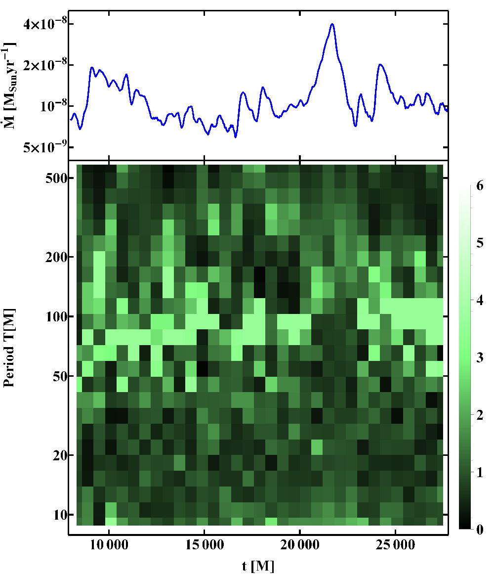
We characterize presence of the oscillations and stability of the oscillation period by a spectrogram in Figure 5. The spectrogram indicates that most of the time oscillations with a period $T=90-100M$ are present. However, no oscillations occur around time $t=22,000M$, when the accretion rate peaks due to weaker magnetic field.

Here we report the QPOs in the simulated SgrA* light curves for models based on the state-of-the-art 3D GRMHD simulations of the magnetically choked RIAFs. The minimization procedure produces a fit with $\chi^{2}/{\rm dof}=1.55$ for ${\rm dof}=9$ to the mean polarized sub-mm source spectrum. The correspondent simulated total flux light curve shows regular oscillations with the period $T\approx 100M\approx 35$ min and the amplitude $\Delta F\approx 0.15$ Jy at $230$ GHz. Less regular fluctuations with $\Delta F\approx 0.2$ Jy are seen at $857$ GHz. Weaker oscillations with $\Delta F\approx 0.05$ Jy are seen at $87$ GHz, which probes the optically thick emission from $\sim 10M$ radius. The LP fraction exhibits periodic modulations at $50\%$ relative level, but the absolute LP flux amplitude is only about $\Delta F_{LP}\approx 0.06$ Jy. The QPOs are significant above $3\sigma$ in the total flux light curves for all tested inclination angles $10^{\circ},$ $37^{\circ},$ and $80^{\circ}$ and frequencies $87$ GHz, $230$ GHz, and $857$ GHz, while the LP fraction shows less prominent QPOs at $87$ GHz and in a face-on case.

Our main $T\approx 35$ min period is longer than the claimed SgrA* observed period $17-20$ min, while the simulated periods $T=6-9$ min in Dolence et al. [11] are shorter. Their simulation has the same BH spin $a_{*}=0.9375$ as does our simulation, but the simulation by Dolence et al. [11] reaches a relatively weak BH horizon magnetic flux and produces a thinner disk with height-to-radius ratio of $H/R\sim 0.2$. The resultant MRI-dominated accretion flow has a Keplerian rotation and shorter QPO periods. They did not identify their QPO mechanism, although they noted their turbulence is unresolved [43] and this might lead to artificial QPOs [22]. Our MCAF model has a sub-Keplerian rotation and the QPOs driven by the interaction of the disk with the rotating BH magnetosphere [25] that leads to longer periods. Our relatively thick disk with $H/R\sim 0.6$ is expected for a RIAF, and our simulations resolve well the disk turbulence [30] suggesting the QPOs are robust. Based upon these works, SgrA* QPOs might be explained by $a_{*}=0.9375$ with an intermediate gas rotation rate, magnetization, or $H/R$.

Flow cooling, whose marginal importance for SgrA* was suggested by Drappeau et al. [12], can self-consistently choose the disk thickness $H/R$ in simulations. In MCAFs, the steady-state BH horizon magnetic flux has a positive correlation with $H/R$ [30], so cooling can lead to more Keplerian rotation and a weaker magnetosphere, and then the QPO period from MCAFs could be comparable to claimed for SgrA*.

We showed that the QPOs, though highly significant, have a maximum sub-mm amplitude of $5\%$ or $\Delta F\sim 0.15$ Jy. Low sensitivity and low sampling rate of current sub-mm instruments might prohibit observational detection of such oscillations [26]. The SMA achieves $5\%$ accuracy and samples every $10$ min at $1.3$ mm with a correspondent $20$ min Nyquist period [28]. A weak signal with $T\sim 30$ min period is readily masked by aliasing and noise in the SMA data. The total flux QPO amplitude $\Delta F\approx 0.15$ Jy is larger than the LP flux amplitude $\Delta F\approx 0.06$ Jy. However, the observational error of the total flux can also be larger. The SMA measures the LP flux to the leakage level of $\sim 0.3\%=9$ mJy, while the total flux is measured to $\sim 0.7\%=20$ mJy due to calibration uncertainties [27]. Then it is about equally difficult to detect the total flux oscillations and the LP flux oscillations.

The ALMA gives more hope in detecting SgrA* sub-mm QPOs. It covers a wide frequency range $84-720$ GHz, has a collecting area of $\sim 7\times 10^{3}{\rm m}^{2}$ about $30$ times that of the SMA, and can sample every few minutes [4]. The ALMA observations of SgrA* will have a flux error under $0.05$ Jy, which is enough to reveal the predicted oscillations were they present on an observation night. As our modeling indicates, the QPOs are absent when the magnetic field is weak due to destruction by magnetic field reversals. The future implementation of the Event Horizon Telescope may allow to measure the QPOs in the source size variations [8]. The anticipated brighter state of SgrA* [33] after the cloud infall may alter our predictions: at a constant $\nu$ the flux increase is compensated by the lower fractional level of the QPOs due to the higher optical depth.

References

- [1] Abramowicz, M. A., Karas, V., Kluzniak, W., Lee, W. H., & Rebusco, P. 2003, PASJ, 55, 467
- [2] Abramowicz, M. A., & Kluźniak, W. 2001, A&A, 374, L19
- [3] Blandford, R. D., & Znajek, R. L. 1977, MNRAS, 179, 433
- [4] Brown, R. L., Wild, W., & Cunningham, C. 2004, Advances in Space Research, 34, 555
- [5] Chan, C.-k., Liu, S., Fryer, C. L., Psaltis, D., Özel, F., Rockefeller, G., & Melia, F. 2009, ApJ, 701, 521
- [6] Dexter, J., Agol, E., Fragile, P. C., & McKinney, J. C. 2010, ApJ, 717, 1092
- [7] Do, T., Ghez, A. M., Morris, M. R., Yelda, S., Meyer, L., Lu, J. R., Hornstein, S. D., & Matthews, K. 2009, ApJ, 691, 1021
- [8] Doeleman, S. S., Fish, V. L., Broderick, A. E., Loeb, A., & Rogers, A. E. E. 2009, ApJ, 695, 59
- [9] Doeleman, S. S., et al. 2008, Nature, 455, 78
- [10] Dolence, J. C., Gammie, C. F., Mościbrodzka, M., & Leung, P. K. 2009, ApJS, 184, 387
- [11] Dolence, J. C., Gammie, C. F., Shiokawa, H., & Noble, S. C. 2012, ApJ, 746, L10
- [12] Drappeau, S., Dibi, S., Dexter, J., Markoff, S., & Fragile, P. C. 2013, MNRAS, 431, 2872
- [13] Falanga, M., Melia, F., Tagger, M., Goldwurm, A., & Bélanger, G. 2007, ApJ, 662, L15
- [14] Falcke, H., Körding, E., & Markoff, S. 2004, A&A, 414, 895
- [15] Gammie, C. F., McKinney, J. C., & Tóth, G. 2003, ApJ, 589, 444
- [16] Genzel, R., Schödel, R., Ott, T., Eckart, A., Alexander, T., Lacombe, F., Rouan, D., & Aschenbach, B. 2003, Nature, 425, 934
- [17] Ghez, A. M., et al. 2008, ApJ, 689, 1044
- [18] Gierliński, M., Middleton, M., Ward, M., & Done, C. 2008, Nature, 455, 369
- [19] Gillessen, S., Eisenhauer, F., Trippe, S., Alexander, T., Genzel, R., Martins, F., & Ott, T. 2009, ApJ, 692, 1075
- [20] Hamaus, N., Paumard, T., Müller, T., Gillessen, S., Eisenhauer, F., Trippe, S., & Genzel, R. 2009, ApJ, 692, 902
- [21] Henisey, K. B., Blaes, O. M., & Fragile, P. C. 2012, ApJ, 761, 18
- [22] Henisey, K. B., Blaes, O. M., Fragile, P. C., & Ferreira, B. T. 2009, ApJ, 706, 705
- [23] Kato, S. 2001, PASJ, 53, 1
- [24] Kato, Y. 2004, PASJ, 56, 931
- [25] Li, L.-X., & Narayan, R. 2004, ApJ, 601, 414
- [26] Marrone, D. P. 2006, PhD thesis, Harvard University
- [27] Marrone, D. P., Moran, J. M., Zhao, J.-H., & Rao, R. 2007, ApJ, 654, L57
- [28] Marrone, D. P., et al. 2008, ApJ, 682, 373
- [29] Mauerhan, J. C., Morris, M., Walter, F., & Baganoff, F. K. 2005, ApJ, 623, L25
- [30] McKinney, J. C., Tchekhovskoy, A., & Blandford, R. D. 2012, MNRAS, 423, 3083
- [31] Miyoshi, M., Shen, Z.-Q., Oyama, T., Takahashi, R., & Kato, Y. 2011, PASJ, 63, 1093
- [32] Mościbrodzka, M., Gammie, C. F., Dolence, J. C., Shiokawa, H., & Leung, P. K. 2009, ApJ, 706, 497
- [33] Mościbrodzka, M., Shiokawa, H., Gammie, C. F., & Dolence, J. C. 2012, ApJ, 752, L1
- [34] Nowak, M. A., & Wagoner, R. V. 1991, ApJ, 378, 656
- [35] Papadakis, I. E., & Lawrence, A. 1993, MNRAS, 261, 612
- [36] Penna, R. F., McKinney, J. C., Narayan, R., Tchekhovskoy, A., Shafee, R., & McClintock, J. E. 2010, MNRAS, 408, 752
- [37] Reis, R. C., Miller, J. M., Reynolds, M. T., Gültekin, K., Maitra, D., King, A. L., & Strohmayer, T. E. 2012, Science, 337, 949
- [38] Remillard, R. A., & McClintock, J. E. 2006, Ann. Rev. Astron. Astr., 44, 49
- [39] Schnittman, J. D., Krolik, J. H., & Hawley, J. F. 2006, ApJ, 651, 1031
- [40] Shcherbakov, R. V., & Baganoff, F. K. 2010, ApJ, 716, 504
- [41] Shcherbakov, R. V., & Huang, L. 2011, MNRAS, 410, 1052
- [42] Shcherbakov, R. V., Penna, R. F., & McKinney, J. C. 2012, ApJ, 755, 133
- [43] Shiokawa, H., Dolence, J. C., Gammie, C. F., & Noble, S. C. 2012, ApJ, 744, 187
- [44] Stone, J. M., & Gardiner, T. 2007, ApJ, 671, 1726
- [45] Tagger, M., & Melia, F. 2006, ApJ, 636, L33
- [46] Timmer, J., & Koenig, M. 1995, A&A, 300, 707
- [47] Trippe, S., Paumard, T., Ott, T., Gillessen, S., Eisenhauer, F., Martins, F., & Genzel, R. 2007, MNRAS, 375, 764
- [48] van der Klis, M. 2000, ARA&A, 38, 717
- [49] Wagoner, R. V. 2008, New Astronomy Reviews, 51, 828
- [50] Yusef-Zadeh, F., Wardle, M., Miller-Jones, J. C. A., Roberts, D. A., Grosso, N., & Porquet, D. 2011, ApJ, 729, 44