On the Minimax Capacity Loss
Under Sub-Nyquist Universal Sampling

In various scenarios, sampling above the Nyquist rate is not necessary for preserving signal information in the sense that it generates a discrete-time sufficient statistic, provided that certain signal structures are appropriately exploited [2, 3]. Take multiband signals for example, that reside within several subbands over a wide spectrum. If the spectral support is known, then the sampling rate necessary for perfect signal reconstruction is the spectral occupancy, termed the Landau rate [4]. Such signals admit perfect recovery when sampled at rates approaching the Landau rate, assuming appropriately chosen sampling sets (e.g. [5, 6]). Inspired by recent “compressed sensing” [7, 8, 9] ideas, spectrum-blind sub-Nyquist samplers have also been developed for multiband signals [10]. Two of the most widely used modules employed in the sampler designs are filter banks and periodic modulation [11, 12, 13, 10]. These sampling-theoretic works, however, were not based on capacity as a metric in the sampler design.

On the other hand, the Shannon-Nyquist sampling theorem has frequently been invoked to investigate the capacity of analog waveform channels (e.g. [14, 15]). The effects upon capacity of oversampling have been investigated as well in the presence of quantization [16, 17]. However, none of these works considered the effect of undersampling upon capacity. Another recent line of work [18] investigated the tradeoff between sparse coding and subsampling in AWGN channels, but did not consider capacity-achieving input distributions.

Our recent work [19, 1] established a new framework for investigating the capacity of LTI Gaussian channels under a broad class of sub-Nyquist sampling strategies, including filter-bank and modulation-bank sampling and, more generally, time-preserving sampling. We demonstrated that sampling with a filter bank is sufficient to approach maximum capacity, assuming that perfect channel state information (CSI) is available at both the receiver and the transmitter. In many practical scenarios, however, the active frequency set available for communications might be changing over time, like in cognitive radio networks where the spectral subbands available to cognitive users are varying over time. To the best of our knowledge, no prior work has investigated, from a capacity perspective, a channel-blind sub-Nyquist sampling paradigm in the absence of subband occupancy information.

Finally, the effect of undersampling has been explored from a source coding perspective as well. For instance, the fundamental rate-distortion function of Gaussian sources has been determined under sub-Nyquist sampling with filtering [20], revealing that the alias suppressing sampler design achieves the optimal rate distortion function. For the case where the input source signals are sparse, the recent work [21] characterized the rate-distortion function under independent and memoryless random sampling. The main results and techniques presented herein might potentially extend to these source coding settings to quantify the rate loss caused by spectral-blind sampling design.

We consider a frequency-flat multiband channel model and the class of sampling systems with filter banks and periodic modulation. For this model, our main contributions are summarized as follows.

• •

  We derive a lower bound (Theorem 2) on the minimax sampled information rate loss (defined in Section II) incurred due to the lack of channel occupancy information, under super-Nyquist universal sampling. This minimax lower limit depends almost only on the band sparsity factor and the undersampling factor, modulo some residual terms that vanish when SNR and $n$ increase.

• •

  We characterize in Theorem 3 the sampled information rate loss under a class of sampling systems with periodic modulation and low-pass filters with passband $\left[0,W/n\right]$, when the Fourier coefficients of the modulation waveforms are generated in an i.i.d. Gaussian fashion (termed Gaussian sampling). We demonstrate that with exponentially high probability, the resulting sampled information rate loss matches the lower bound given in Theorem 2 uniformly over all possible subband occupancy. This implies that random sampling strategies are minimax-optimal in terms of a universal sampling design.

• •

  The power of random sampling arises due to sharp concentration of spectral measures of large random matrices [23]. To establish Theorem 3, we derive measure concentration of several log-determinant functions for i.i.d. Gaussian ensembles, which might be of independent interest for other works involving log-determinant metrics.

The remainder of this paper is organized as follows. In Section II we introduce our system model of multiband Gaussian channels. A metric called sampled information rate loss, and a minimax sampler, are defined with respect to sampled channel capacity. We then determine in Section III the minimax information rate loss. Specifically, we develop lower bounds on the minimax information rate loss in Section III-A. The achievability is treated in Section III-B. Besides, we derive measure concentration of several log-determinant functions in Section IV-C. Section V-A summarizes the key observation and implications from our results. Section VI closes the paper with a short summary of our findings and potential future directions.

Denote by $\mathcal{H}(\beta):=-\beta\log\beta-(1-\beta)\log(1-\beta)$ the binary entropy function. The standard notation $f(n)=\mathcal{O}\left(g(n)\right)$ means there exists a constant $c>0$ such that $\left|f(n)\right|\leq c|g(n)|$, $f(n)=\Theta\left(g(n)\right)$ means there exist constants $c_{1},c_{2}>0$ such that $c_{1}|g(n)|\leq|f(n)|\leq c_{2}|g(n)|$, $f(n)=\omega\left(g(n)\right)$ means that $\lim_{n\rightarrow\infty}\frac{g(n)}{f(n)}=0$, and $f(n)=o\left(g(n)\right)$ indicates that $\lim_{n\rightarrow\infty}\frac{f(n)}{g(n)}=0$. For a matrix $\boldsymbol{A}$, we use $\boldsymbol{A}_{i*}$ and $\boldsymbol{A}_{*i}$ to denote the $i$th row and $i$th column of $\boldsymbol{A}$, respectively. We let $[n]$ denote the set $\left\{1,2,\cdots,n\right\}$, and write ${[n]\choose k}$ for the set of all $k$-element subsets of $\left\{1,2,\cdots,n\right\}$. We also use $\text{card}\left(\mathcal{A}\right)$ to denote the cardinality of a set $\mathcal{A}$. Let $\boldsymbol{W}$ be a $p\times p$ random matrix that can be expressed as $\boldsymbol{W}=\Sigma_{i=1}^{n}\boldsymbol{Z}_{i}\boldsymbol{Z}_{i}^{\top}$, where $\boldsymbol{Z}_{i}\sim\mathcal{N}\left(0,\boldsymbol{\Sigma}\right)$ are jointly independent Gaussian vectors. Then $\boldsymbol{W}$ is said to have a central Wishart distribution with $n$ degrees of freedom and scale matrix $\boldsymbol{\Sigma}$, denoted by $\boldsymbol{W}\sim\mathcal{W}_{p}(n,\boldsymbol{\Sigma})$. Our notation is summarized in Table I.

We consider a multiband Gaussian channel of total bandwidth $W$, and it is divided into $n$ continuous subbands¹¹ 1 Note that in practice, $n$ is typically a large number. For instance, the number of subcarriers ranges from 128 to 2048 in LTE [24, 25]. each of bandwidth $W/n$. A state $\boldsymbol{s}\in{[n]\choose k}$ is generated, which dictates the channel support. For ease of presentation, the present work focuses on the frequency-flat channel model, which suffices to capture the essence of our findings. Specifically, given a state $\boldsymbol{s}$, the channel is assumed to be an LTI filter with impulse response $h_{\boldsymbol{s}}(t)$ and frequency response

A transmit signal $x(t)$ with a power constraint $P$ is passed through this multiband channel, yielding a channel output

where $\eta(t)$ is stationary zero-mean Gaussian noise with power spectral density $\mathcal{S}_{\eta}\left(f\right)\equiv 1$. It is assumed throughout that the knowledge of $H$ and $\mathcal{S}_{\eta}$ are available at both the transmitter and the receiver, while the state $\boldsymbol{s}$ is known only at the transmitter. The results derived herein can be extended to more general frequency selective channels with optimal power control. These extensions are described in more details in Section V-B and derived in [26].

We aim to design a sampler that operates below the Nyquist rate (i.e. the channel bandwidth $W$). In particular, the present work focuses on the class of filter-bank and modulation-bank sampling systems, which subsumes the most widely used sampling mechanisms in practice.

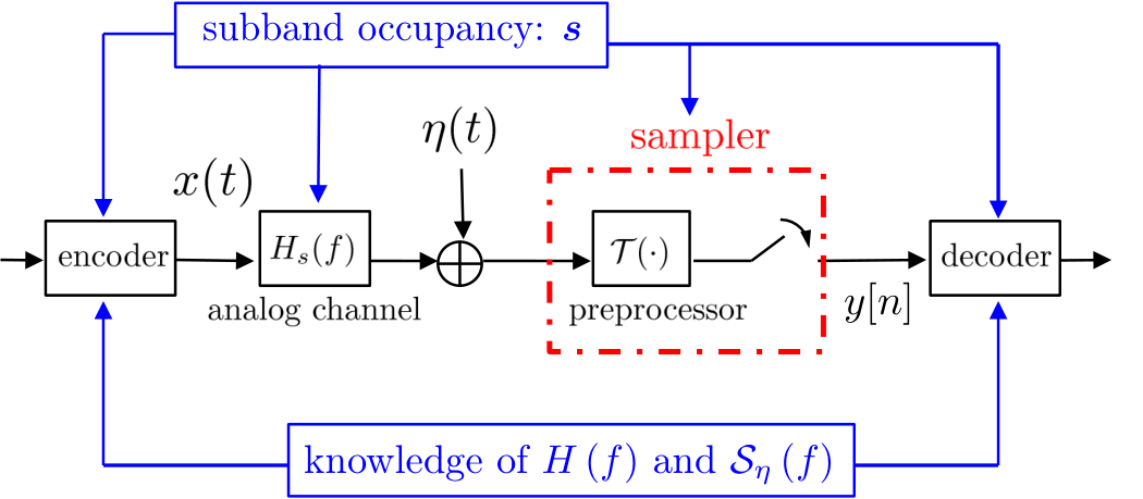
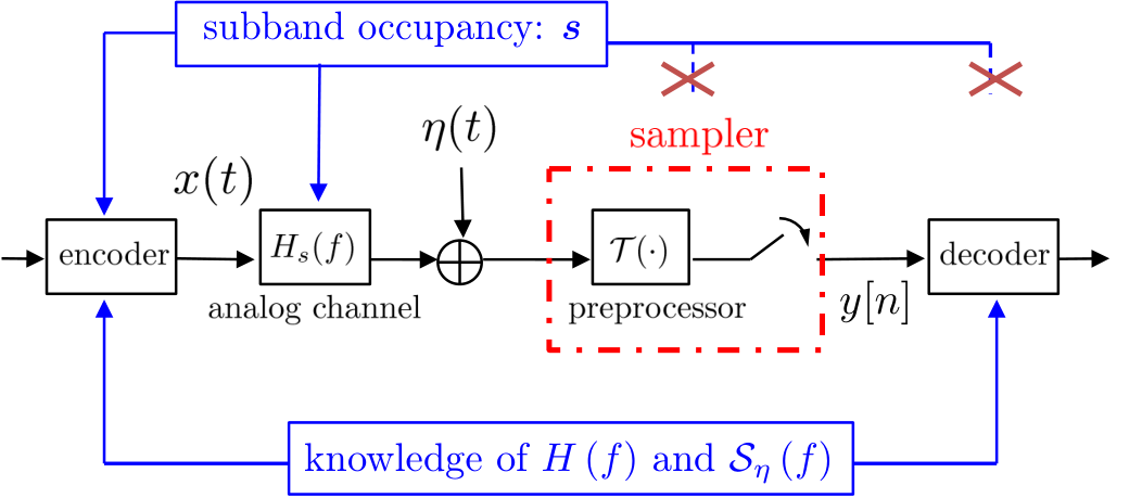
As was shown in [1], the optimal sampling mechanism for a given LTI channel with perfect CSI extracts out the frequency set with the highest SNR and hence suppresses aliasing. Such an alias-suppressing sampler may result in a very low capacity for some channel support. In this paper, we desire a sampler that operates independent of the instantaneous subband occupancy, and our objective is to design a single linear sampling system that incurs minimal information rate loss across all possible channel occupancy. In particular, the information rate loss we consider is the gap between the capacity under sampling with and without spectral occupancy (i.e. Fig. 2(a) vs. Fig. 2(b)).

We need to demonstrate that the minimax sampled information rate loss under any channel-independent sampler cannot be lower than (17)-(19) in respective regimes. This is given by the theorem below.

For the entire sub-Nyquist regime, the lower bounds we derive are tantamount to some constants dependent only on $\alpha$ and $\beta$, except for some residual terms that vanish when the number $n$ of subbands and the SNR tend to infinity. More precisely, when $\alpha\neq\beta$, one has $\Lambda,\Psi=\mathcal{O}\left(\frac{1}{\small\mathsf{SNR}}\right)$, and hence these residuals are at most the order of $\mathcal{O}\left(\frac{1}{\small\mathsf{SNR}}+\frac{\log n}{n}\right)$. In contrast, in the Landau-rate regime ($\alpha=\beta$), the residual term is bounded in magnitude by $\frac{2}{\sqrt{\small\mathsf{SNR}}}+\frac{\log\left(n+1\right)}{n}$. In fact, the term $\mathcal{O}\left(\frac{\log n}{n}\right)$ arises when using the entropy function to approximate the rate of binomial coefficients, while an additional approximation loss $\mathcal{O}\left(\frac{1}{\small\mathsf{SNR}}\right)$ occurs when employing $\log\mathsf{SNR}$ to approximate $\log\left(1+\mathsf{SNR}\right)$.

In general, it is computationally intractable to find a deterministic solution to approach the minimax limits by solving a numerical optimization program. Fortunately, when $n$ and SNR are both large, simple random sampling strategies suffice in approaching the minimax information rate loss limits uniformly under all channel occupancy. The achievability result is formally stated in the following theorem.

Theorem 3 indicates that Gaussian sampling approaches the minimax information rate loss (which is about $\frac{1}{2}\mathcal{H}(\beta)-\frac{1}{2}\alpha\mathcal{H}\left(\frac{\beta}{\alpha}\right)$ per Hertz) to within a small gap. In fact, with exponentially high probability, the sampled information rate loss is almost equivalent to the minimax limit uniformly across all states $\boldsymbol{s}\in{[n]\choose k}$, as will be shown later.

Recall that $\boldsymbol{Q}^{\text{w}}\boldsymbol{Q}^{\text{w}*}=\boldsymbol{I}$, and that $\boldsymbol{B}_{\boldsymbol{s}}$ represents the $m\times k$ submatrix of $\boldsymbol{B}$ with columns coming from the index set $\boldsymbol{s}$. The following theorem investigates the properties of $\log\det\left(\epsilon\boldsymbol{I}_{k}+\boldsymbol{B}_{\boldsymbol{s}}^{*}\boldsymbol{B}_{\boldsymbol{s}}\right)$ for any $m\times n$ matrix $\boldsymbol{B}$ that has orthonormal rows.

Theorem 4 together with (27) suggests that

which completes the proof of Theorem 2.

One of the key ingredients in establishing Theorem 4 is to demonstrate that the sum

is a constant independent of the matrix $\boldsymbol{B}$, as long as $\boldsymbol{B}$ has orthonormal rows. Consequently, in order to maximize $\min_{\boldsymbol{s}}\det\left(\epsilon\boldsymbol{I}+\boldsymbol{B}_{\boldsymbol{s}}^{*}\boldsymbol{B}_{\boldsymbol{s}}\right)$, one would wish to find a matrix $\boldsymbol{B}$ such that $\det\left(\epsilon\boldsymbol{I}+\boldsymbol{B}_{\boldsymbol{s}}^{*}\boldsymbol{B}_{\boldsymbol{s}}\right)$ are almost identical over all $\boldsymbol{s}$. When translated to the language of channel capacity, this observation suggests that an ideal minimax sampling method should be able to achieve (almost) equivalent information rate loss uniformly over all states $\boldsymbol{s}$, for which random sampling becomes a natural candidate due to sharp concentration of measures.

When it comes to the achievability part, the major step is to quantify $\log\det(\epsilon\boldsymbol{I}+(\boldsymbol{M}\boldsymbol{M}^{\top})^{-1}\boldsymbol{M}_{\boldsymbol{s}}\boldsymbol{M}_{\boldsymbol{s}}^{\top})$ for every $\boldsymbol{s}\in{[n]\choose k}$. Interestingly, this quantity can be uniformly controlled due to the concentration of spectral measure of random matrices [23]. This is stated in the following theorem, which demonstrates the optimality of Gaussian sampling mechanisms.

Putting Theorem 5 and Equation (27) together implies that $\forall\boldsymbol{s}\in{[n]\choose k}$,

with exponentially high probability, which establishes Theorem 3. The above achievability bounds are established via the concentration of spectral measure of large random matrices.

As mentioned above, the key machinery in establishing the achievability bounds is to evaluate certain log-determinant functions. In fact, many limiting results for i.i.d. Gaussian ensembles have been derived when studying MIMO fading channels (e.g. [28, 29, 30, 31]), which focus on the first-order limits instead of the convergence rate. Furthermore, the second-order asymptotics and the large deviation for mutual information have also been studied (e.g. [32, 33]) in the asymptotic regime of large $n$. Most of these results focus on a special case of the log-determinant function (i.e. $\log\det(\epsilon\boldsymbol{I}+\frac{1}{n}\boldsymbol{M}\boldsymbol{M}^{\top})$) and suppose that $n$ scales independent of $\epsilon$. On the other hand, the concentration of some log-determinant functions has been studied in the random matrix literature as a key step in establishing universal laws for linear spectral statistics (e.g. [34, Proposition 48]). However, these bounds are only shown to hold with overwhelming probability (i.e. with probability $1-e^{-\omega\left(\log n\right)}$), which are not sharp enough for our purpose. As a result, we provide sharper measure concentration results of log-determinants in this subsection.

One important class of log-determinant functions takes the form of $\frac{1}{n}\log\det\left(\frac{1}{n}\boldsymbol{A}\boldsymbol{A}^{\top}\right)$. The concentration of such functions for i.i.d. rectangular Gaussian matrices is characterized in the following lemmas.

The last log-determinant function considered here takes the form of $\log\det\left(\epsilon\boldsymbol{I}+\boldsymbol{A}^{\top}\boldsymbol{B}^{-1}\boldsymbol{A}\right)$ for some independent random matrices $\boldsymbol{A}$ and $\boldsymbol{B}$, as stated in the following lemma.

As demonstrated in (27), the information rate loss is captured by some logarithmic function. The preceding concentration of measure results will prove useful in determining such a information rate loss metric.

In this subsection, we summarize several key insights from the main theorems.

• (1)

  For the whole sub-Nyquist regime, the minimax information rate loss is captured by several binary entropy functions. When the number of subbands and the SNR are sufficiently large and $\frac{\small\mathsf{SNR}}{n}=o\left(1\right)$, the minimax limits depend almost only on the undersampling factor and the sparsity factor rather than $\left(n,k,m\right)$, which are plotted in Fig. 4. It can be observed from the plot that when sampling above the Landau rate (but below the Nyquist rate), increasing the $\alpha/\beta$ ratio improves the capacity gap, and shrinks the locus. In contrast, when $\alpha<\beta$, increasing $\alpha/\beta$ results in a worse capacity gap. This implies that in the sub-Landau regime, the relative information rate loss is easier to control when $\alpha/\beta$ decreases, although the achievable channel capacity also shrinks. In fact, the information rate loss is the largest under Landau-rate sampling, as illustrated in Fig. 4. Since the capacity under channel-optimized sampling scales as $\Theta\left(W\log\mathsf{SNR}\right)$, our results indicate that the ratio of the minimax information rate loss to the maximum capacity vanishes at a rate $\Theta\left(1/\log\mathsf{SNR}\right)$.

• (2)

  Note that under Landau-rate sampling (i.e. $\alpha=\beta$), the minimax loss is $\frac{1}{2}\mathcal{H}\left(\beta\right)$ (or $\frac{1}{2}\mathcal{H}\left(\alpha\right)$) modulo some residual terms. As a result, if we fix the channel sparsity factor and increase the sampling rate above the Landau rate, then the capacity benefit per unit bandwidth is captured by the term $\frac{1}{2}\alpha\mathcal{H}\left(\beta/\alpha\right)$. On the other hand, if we fix the sampling rate but increase the channel occupancy, then the capacity gain per Hertz one can harvest amounts to $\frac{1}{2}\beta\mathcal{H}\left(\alpha/\beta\right)$. For either case, if $\alpha\rightarrow 1$, the information rate loss per Hertz reduces to

  $$\frac{1}{2}\mathcal{H}\left(\beta\right)-\frac{1}{2}\alpha\mathcal{H}\left(\frac{\beta}{\alpha}\right)=0,$$

  meaning that there is effectively no information rate loss under Nyquist-rate sampling. This agrees with the fact that Nyquist-rate sampling is information preserving.

• (3)

  The information rate loss incurred by Gaussian random sampling meets the minimax limit for Landau-rate sampling uniformly across all states $\boldsymbol{s}$, which reveals that with exponentially high probability, random sampling is optimal in terms of universal sampling design. This arises since the capacity achievable by random sampling exhibits very sharp measure concentration.

• •

  Universality of Random Sampling Schemes Beyond Gaussian Sampling. While the main theorems provided in the present paper focus on Gaussian sampling, we remark that a much broader class of random sampling strategies are also minimax-optimal. This subsumes the class of sampling coefficient matrices $\boldsymbol{M}$ such that its entries are independent sub-Gaussian random variables with matching moments up to the second order. The universality phenomenon that arises in large random matrices (e.g. [35]) suggests that the minimaxity of random sampling matrices does not depend on the particular distribution of the coefficients, although they might affect the convergence rate to some degree. Interested readers are referred to [26] for derivation of these results and associated insights.

• •

  Beyond Frequency-Flat Channels and Uniform Power Allocation. The present paper concentrates on the frequency-flat channel models for simplicity of presentation. Note, however, that the main results derived herein can be readily extended to more general frequency-varying channels. Specifically, suppose that the information rate loss metric is defined as the gap of achievable rates under universal sampling relative to channel-optimized sampling (both employing optimal power allocation). Then as long as the peak-to-average SNR

  $$\frac{\sup_{f\in\left[0,W\right]}\left|H\left(f\right)\right|^{2}/\mathcal{S}_{\eta}\left(f\right)}{\frac{1}{W}\int_{0}^{W}\left|H\left(f\right)\right|^{2}/\mathcal{S}_{\eta}\left(f\right)}$$

  is bounded, all results presented in this paper still hold, except for some additional gap on the order of $\mathcal{O}\left(\frac{1}{\small\mathsf{SNR}_{\min}}\right)$, where

  $$\mathsf{SNR}_{\min}:=\inf_{f\in\left[0,W\right]}\frac{P}{\min\left\{\alpha,\beta\right\}W}\frac{\left|H\left(f\right)\right|^{2}}{\mathcal{S}_{\eta}\left(f\right)}.$$

  A proof of this result and derivation of the optimal power allocation is provided in [26].

References

• [1] Y. Chen, Y. C. Eldar, and A. J. Goldsmith, “Channel capacity under sub-Nyquist nonuniform sampling,” IEEE Transactions on Information Theory, vol. 60, no. 8, pp. 4739 – 4756, August 2014.
• [2] P. L. Butzer and R. L. Stens, “Sampling theory for not necessarily band-limited functions: A historical overview,” SIAM Review, vol. 34, no. 1, pp. 40–53, 1992.
• [3] M. Mishali and Y. C. Eldar, “Sub-Nyquist sampling: Bridging theory and practice,” IEEE Signal Processing Magazine, vol. 28, no. 6, pp. 98–124, Nov. 2011.
• [4] H. Landau, “Necessary density conditions for sampling and interpolation of certain entire functions,” Acta Mathematica, vol. 117, pp. 37–52, 1967.
• [5] C. Herley and P. W. Wong, “Minimum rate sampling and reconstruction of signals with arbitrary frequency support,” IEEE Transactions on Information Theory, vol. 45, no. 5, pp. 1555 –1564, Jul. 1999.
• [6] R. Venkataramani and Y. Bresler, “Optimal sub-Nyquist nonuniform sampling and reconstruction for multiband signals,” IEEE Transactions on Signal Processing, vol. 49, no. 10, pp. 2301 –2313, Oct. 2001.
• [7] E. Candes, J. Romberg, and T. Tao, “Robust uncertainty principles: exact signal reconstruction from highly incomplete frequency information,” IEEE Transactions on Information Theory, vol. 52, no. 2, pp. 489–509, Feb. 2006.
• [8] D. L. Donoho, “Compressed sensing,” IEEE Transactions on Information Theory, vol. 52, no. 4, pp. 1289 –1306, April 2006.
• [9] Y. C. Eldar and G. Kutyniok, Compressed Sensing: Theory and Applications. Cambridge University Press Cambridge, 2012, vol. 95.
• [10] M. Mishali and Y. C. Eldar, “From theory to practice: Sub-Nyquist sampling of sparse wideband analog signals,” IEEE Journal of Selected Topics in Signal Processing, vol. 4, no. 2, pp. 375 –391, Apr. 2010.
• [11] A. Papoulis, “Generalized sampling expansion,” IEEE Transactions on Circuits and Systems, vol. 24, no. 11, pp. 652 – 654, Nov 1977.
• [12] Y.-P. Lin and P. Vaidyanathan, “Periodically nonuniform sampling of bandpass signals,” IEEE Transactions on Circuits and Systems II: Analog and Digital Signal Processing, vol. 45, no. 3, pp. 340 –351, Mar. 1998.
• [13] W. A. Gardner, “The spectral correlation theory of cyclostationary time-series,” Signal processing, vol. 11, no. 1, pp. 13–36, 1986.
• [14] M. Medard, “The effect upon channel capacity in wireless communications of perfect and imperfect knowledge of the channel,” IEEE Trans. on Info Theory, vol. 46, no. 3, pp. 933 –946, May. 2000.
• [15] P. Bello, “Characterization of randomly time-variant linear channels,” IEEE Transactions on Communications Systems, vol. 11, no. 4, pp. 360 –393, Dec. 1963.
• [16] S. Shamai, “Information rates by oversampling the sign of a bandlimited process,” IEEE Transactions on Information Theory, vol. 40, no. 4, pp. 1230 –1236, Jul. 1994.
• [17] T. Koch and A. Lapidoth, “Increased capacity per unit-cost by oversampling,” Sep. 2010. [Online]. Available: http://arxiv.org/abs/1008.5393
• [18] M. Peleg and S. Shamai, “On sparse sensing of coded signals at sub-Landau sampling rates,” IEEE 27th Convention of Electrical Electronics Engineers in Israel (IEEEI), pp. 1 –5, Nov. 2012.
• [19] Y. Chen, Y. C. Eldar, and A. J. Goldsmith, “Shannon meets Nyquist: Capacity of sampled Gaussian channels,” IEEE Transactions on Information Theory, vol. 59, no. 8, pp. 4889 – 4914, August 2013.
• [20] A. Kipnis, A. J. Goldsmith, T. Weissman, and Y. C. Eldar, “Distortion-rate function of sub-Nyquist sampled Gaussian sources,” arXiv preprint arXiv:1405.5329, 2014.
• [21] V. Boda and P. Narayan, “Sampling rate distortion,” in IEEE International Symposium on Information Theory (ISIT), June 2014, pp. 3057–3061.
• [22] Y. Chen, A. Goldsmith, and Y. Eldar, “Backing off from infinity: Performance bounds via concentration of spectral measure for random MIMO channels,” IEEE Transactions on Information Theory, vol. 61, no. 1, pp. 366–387, Jan 2015.
• [23] A. Guionnet and O. Zeitouni, “Concentration of the spectral measure for large matrices,” Electronic Communications in Probability, no. 5, pp. 119 –136, 2000.
• [24] A. Ghosh, J. Zhang, R. Muhamed, and J. G. Andrews, Fundamentals of LTE. Pearson Education, 2010.
• [25] “LTE in a nutshell: White paper on physical layer,” 2010.
• [26] Y. Chen, “Subsampling in information theory and data processing,” Ph.D. Thesis, Stanford University, January 2015. [Online]. Available: http://web.stanford.edu/~yxchen/publications/thesis_YChen.pdf
• [27] S. Sesia, I. Toufik, and M. Baker, LTE: the UMTS long term evolution. Wiley Online Library, 2009.
• [28] E. Telatar, “Capacity of multi-antenna Gaussian channels,” European Transactions on Telecommunications, vol. 10, no. 6, pp. 585 – 595, Nov. - Dec. 1999.
• [29] A. Lozano and A. M. Tulino, “Capacity of multiple-transmit multiple-receive antenna architectures,” IEEE Transactions on Information Theory, vol. 48, no. 12, pp. 3117–3128, 2002.
• [30] C.-N. Chuah, D. N. C. Tse, J. M. Kahn, and R. A. Valenzuela, “Capacity scaling in MIMO wireless systems under correlated fading,” IEEE Transactions on Information Theory, vol. 48, no. 3, pp. 637–650, 2002.
• [31] A. M. Tulino and S. Verdu, Random Matrix Theory and Wireless Communications, ser. Foundations and Trends in Communications and Information Theory. Hanover, MA: Now Publisher Inc., 2004.
• [32] W. Hachem, O. Khorunzhiy, P. Loubaton, J. Najim, and L. Pastur, “A new approach for mutual information analysis of large dimensional multi-antenna channels,” IEEE Transactions on Information Theory, vol. 54, no. 9, pp. 3987–4004, 2008.
• [33] P. Kazakopoulos, P. Mertikopoulos, A. L. Moustakas, and G. Caire, “Living at the edge: A large deviations approach to the outage MIMO capacity,” IEEE Transactions on Information Theory, vol. 57, no. 4, pp. 1984–2007, 2011.
• [34] T. Tao and V. Vu, “Random matrices: Universality of local spectral statistics of non-Hermitian matrices,” June 2012. [Online]. Available: arxiv.org/pdf/1206.1893.pdf
• [35] ——, “Random covariance matrices: Universality of local statistics of eigenvalues,” The Annals of Probability, vol. 40, no. 3, pp. 1285 – 1315, 2012.
• [36] A. E. Gamal and Y. H. Kim, Network Information theory. Cambridge University Press, 2011.
• [37] R. A. Horn and C. R. Johnson, Matrix analysis. Cambridge University Press, 1985.
• [38] T. M. Cover and J. A. Thomas, Elements of information theory. John Wiley & Sons, 2012.
• [39] T. Tao, Topics in Random Matrix Theory, ser. Graduate Studies in Mathematics. Providence, Rhode Island: American Mathematical Society, 2012.
• [40] A. Edelman, “The probability that a random real Gaussian matrix has kk real eigenvalues, related distributions, and the circular law,” Journal of Multivariate Analysis, vol. 60, no. 2, pp. 203–232, 1997.
• [41] Y. Fujikoshi, V. V. Ulyanov, and R. Shimizu, Multivariate Statistics: High-dimensional and Large-sample Approximations, ser. Wiley Series in Probability and Statistics. Hoboken, New Jersey: Wiley, 2010.
• [42] R. Vershynin, “Introduction to the non-asymptotic analysis of random matrices,” Compressed Sensing, Theory and Applications, pp. 210 – 268, 2012.
• [43] Z. Chen and J. J. Dongarra, “Condition numbers of Gaussian random matrices,” SIAM Journal on Matrix Analysis and Applications, vol. 27, no. 3, pp. 603–620, July 2005.
Yuxin Chen (S’09) received the B.S. in Microelectronics with High Distinction from Tsinghua University in 2008, the M.S. in Electrical and Computer Engineering from the University of Texas at Austin in 2010, the M.S. in Statistics from Stanford University in 2013, and the Ph.D. in Electrical Engineering from Stanford University in 2015. He joins the Department of Electrical Engineering at Princeton University as an assistant professor in February 2017. His research interests include mathematical optimization, information theory, high-dimensional statistics, and statistical learning.
Andrea J. Goldsmith (S’90-M’93-SM’99-F’05) is the Stephen Harris professor in the School of Engineering and a professor of Electrical Engineering at Stanford University. She was previously on the faculty of Electrical Engineering at Caltech. Her research interests are in information theory and communication theory, and their application to wireless communications and related fields. She co-founded and serves as Chief Scientist of Accelera, Inc., and previously co-founded and served as CTO of Quantenna Communications, Inc. She has also held industry positions at Maxim Technologies, Memorylink Corporation, and AT&T Bell Laboratories. Dr. Goldsmith is a Fellow of the IEEE and of Stanford, and she has received several awards for her work, including the IEEE Communications Society and Information Theory Society joint paper award, the IEEE Communications Society Best Tutorial Paper Award, the National Academy of Engineering Gilbreth Lecture Award, the IEEE ComSoc Communications Theory Technical Achievement Award, the IEEE ComSoc Wireless Communications Technical Achievement Award, the Alfred P. Sloan Fellowship, and the Silicon Valley/San Jose Business Journal’s Women of Influence Award. She is author of the book “Wireless Communications” and co-author of the books “MIMO Wireless Communications” and “Principles of Cognitive Radio,” all published by Cambridge University Press. She received the B.S., M.S. and Ph.D. degrees in Electrical Engineering from U.C. Berkeley. Dr. Goldsmith has served on the Steering Committee for the IEEE Transactions on Wireless Communications and as editor for the IEEE Transactions on Information Theory, the Journal on Foundations and Trends in Communications and Information Theory and in Networks, the IEEE Transactions on Communications, and the IEEE Wireless Communications Magazine. She participates actively in committees and conference organization for the IEEE Information Theory and Communications Societies and has served on the Board of Governors for both societies. She has also been a Distinguished Lecturer for both societies, served as President of the IEEE Information Theory Society in 2009, founded and chaired the student committee of the IEEE Information Theory society, and chaired the Emerging Technology Committee of the IEEE Communications Society. At Stanford she received the inaugural University Postdoc Mentoring Award, served as Chair of Stanfords Faculty Senate in 2009 and currently serves on its Faculty Senate and on its Budget Group.
Yonina C. Eldar (S’98-M’02-SM’07-F’12) received the B.Sc. degree in physics and the B.Sc. degree in electrical engineering both from Tel-Aviv University (TAU), Tel-Aviv, Israel, in 1995 and 1996, respectively, and the Ph.D. degree in electrical engineering and computer science from the Massachusetts Institute of Technology (MIT), Cambridge, in 2002. From January 2002 to July 2002, she was a Postdoctoral Fellow at the Digital Signal Processing Group at MIT. She is currently a Professor in the Department of Electrical Engineering at the Technion-Israel Institute of Technology, Haifa and holds the The Edwards Chair in Engineering. She is also a Research Affiliate with the Research Laboratory of Electronics at MIT and a Visiting Professor at Stanford University, Stanford, CA. Her research interests are in the broad areas of statistical signal processing, sampling theory and compressed sensing, optimization methods, and their applications to biology and optics. Dr. Eldar was in the program for outstanding students at TAU from 1992 to 1996. In 1998, she held the Rosenblith Fellowship for study in electrical engineering at MIT, and in 2000, she held an IBM Research Fellowship. From 2002 to 2005, she was a Horev Fellow of the Leaders in Science and Technology program at the Technion and an Alon Fellow. In 2004, she was awarded the Wolf Foundation Krill Prize for Excellence in Scientific Research, in 2005 the Andre and Bella Meyer Lectureship, in 2007 the Henry Taub Prize for Excellence in Research, in 2008 the Hershel Rich Innovation Award, the Award for Women with Distinguished Contributions, the Muriel & David Jacknow Award for Excellence in Teaching, and the Technion Outstanding Lecture Award, in 2009 the Technion’s Award for Excellence in Teaching, in 2010 the Michael Bruno Memorial Award from the Rothschild Foundation, and in 2011 the Weizmann Prize for Exact Sciences. In 2012 she was elected to the Young Israel Academy of Science and to the Israel Committee for Higher Education, and elected an IEEE Fellow. In 2013 she received the Technion’s Award for Excellence in Teaching, the Hershel Rich Innovation Award, and the IEEE Signal Processing Technical Achievement Award. She received several best paper awards together with her research students and colleagues. She received several best paper awards together with her research students and colleagues. She is the Editor in Chief of Foundations and Trends in Signal Processing. In the past, she was a Signal Processing Society Distinguished Lecturer, member of the IEEE Signal Processing Theory and Methods and Bio Imaging Signal Processing technical committees, and served as an associate editor for the IEEE Transactions On Signal Processing, the EURASIP Journal of Signal Processing, the SIAM Journal on Matrix Analysis and Applications, and the SIAM Journal on Imaging Sciences.