Testing the spin-cutoff parameterization with shell-model calculations
Abstract
The nuclear level density, an important input to Hauser-Feshbach calculations, depends not only on excitation energy but also on angular momentum . The -dependence of the level density at fixed excitation energy is usually parameterized via the spin-cutoff factor . We carefully test the statistical accuracy of this parameterization for a large number of spectra computed using semi-realistic interactions in the interacting shell model, with a nonlinear least-squares fit of and finding the error bar in . The spin-cutoff parameterization works well as long as there are enough states to be statistical. In turn, the spin-cutoff factor can be related to the average value of at a fixed excitation energy, and we briefly investigate extracting from a thermal calculation such as one might do via Monte Carlo.
pacs
21.10.Ma,21.60.CsI Introduction
An important input into compound nuclear reactions such as statistical neutron capture is the level density[1]. The level density is deceptively simple: the number of levels per unit of excitation energy. But when thousands or millions of states or more are involved, as in the statistical regime, experimental measurement becomes challenging and theoretical calculations are also difficult if not intractable. Because of this the level density is one of the most uncertain inputs into reaction calculations [2].
(Note: one should be careful to distinguish between the level density, which does not include the degeneracy in , and the state density which does include the degeneracy in .)
For calculation of statistical neutron capture rates one needs not only the density of levels as a function of excitation energy but also as a function of parity and angular momentum . While there are different parameterizations for the level density , such as the back-shifted Fermi-gas [3, 4, 5] or constant temperature [4], for the dependence on the parameterization [6]
| (1) |
is universally used, where is called the spin-cutoff factor. (This normalization is for the level density; for the state density the spin-cutoff parameterization has a different normalization, found below in Eq. (4).)
A number of other works have investigated the spin distribution of levels, both experimentally [7, 8, 9, 10] and theoretically [11, 12, 13, 14]. While these papers have compared the actual spin distribution against the spin-cutoff parameterization, in this paper we focus on quantifying the statistical goodness of the spin-cutoff parameterization by computing the error bars on the spin-cutoff factor.
Towards this end, we have generated a number of theoretical nuclear spectra, as described in more detail in Section II. We then put the data into energy bins and, in each energy bin, did a nonlinear least-squares fit for using Eq. (1), including deriving the error bars on . The fitting methodology and results we give in Section III.
In general we find the unsuprising but gratifying result that the spin-cutoff parameterization does a good job of describing the spin distribution, and that the error bars on decrease as the number of levels in a bin increase. If Eq. (1) were wrong, the error bars would not decrease systematically.
Because Eq. (1) has only the one parameter , it is tempting to try to extract the spin-cutoff factor directly rather than fitting it, for example relating to the average value of at a given excitation energy. This would be useful in particular for Monte Carlo calculations such as the so-called shell-model Monte Carlo (SMMC) [15, 16] from which state densities can be extracted [13, 14, 17, 18, 19, 20, 21, 22]; although a -projected versions of SMMC has been developed [13, 14], it is computationally very intensive. By contrast, it is relatively easy to compute thermally-averaged expectation values of operators such as in SMMC. Because one needs the average as a function of excitation energy and not temperature, one needs to extract the energy-averaged from thermally-weighted values, in the same way one inverts the Laplace transform to extract the state density from the thermal partition function. This we discuss in Section IV.
II Shell-model framework
We work in the framework of the configuration-interaction shell model [23, 24, 25]. Here one defines a finite single-particle space and has as input single-particle energies and two-body matrix elements. We use semi-realistic/semi-phenomenological matrix elements, meaning each interaction starts from realistic fits to scattering data, is then renormalized, and finally tuned to reproduce binding energies and spectra for a specified mass region (see [23, 26] for details of methodology).
All model spaces assume some inert core and valence particles. The three model spaces we work in and their interactions are:
sd, or the 1-- valence space, assuming an inert 16O core; the interaction is the universal -interaction ‘B,’ or USDB [26];
pf, or the --- valence space, assuming an inert 40Ca core; the interaction is the monopole-modified Kuo-Brown G-matrix interaction version 3G, or KB3G [27, 28];
and finally the ps-d5/2, or --- valence space, assuming an inert 4He core; the interaction is a hybrid of Cohen-Kurath (CK) matrix elements in the shell[29], the older universal interaction of Wildenthal [30] in the - space, and the Millener-Kurath (MK) - cross-shell matrix elements [31]. We leave out the orbit to make calculations tractable. Within the and spaces we use the original spacing of the single-particle energies for the CK and Wildenthal interactions, respectively, but then shift the single-particle energies relative to the -shell single particle energies to place the first state in 16O at approximately MeV above the ground state. The rest of the spectrum, in particular the first excited state, is not very good, but the idea is to have a non-trivial model, not exact reproduction of the spectrum. This model space and interaction allows us to consider model nuclei with both parities and to investigate parity-mixing in the HF state.
Finally, we computed the many-body spectra using the BIGSTICK configuration-interaction diagonalization code [32]. Table 1 lists the nuclides computed and the single-particle spaces used. In this paper we display a representative sample, but graphs for all nuclides in Table 1 are included in the supplemental material [33].
| sd | pf | p-sd5/2 |
|---|---|---|
| 22-27Na | 46-52Ca | 11-13C |
| 24-29Mg | 45-47,49Sc | 14N |
| 26-30Al | 44-47Ti | 16-17O |
| 28-32Si | 46V | 20Ne |
| 30-33P | ||
| 32-34S | ||
| 34-35Cl |
III Results
To analyze the spin distribution of shell-model spectra, we binned the data into 1 MeV bins (our results were insensitive to the size of the bins, as we discuss at the end of this section), and did a non-linear least-squares fit to the Ericson formula using the MPFIT code [35, 34], an implementation of the Levenberg-Marquardt algorithm [36]. The error bar on the least-squares-fit spin-cutoff parameter is just the standard square root of the diagonal of the covariance matrix, which in our case was a trivial matrix. For the purpose of the fit we estimate the error of each -projected density in an energy bin to be the standard counting statistical error, ; bins with are assigned an error of 1. Our initial per degree of freedom, or reduced ,
| (2) |
nearly always fell below 1 and frequently . Because we have only one parameter, overfitting is unlikely; instead we suspect the errors are non-Gaussian, asymmetric (for example, no density can be less than zero) and/or correlated. To obtain a reduced for a given energy bin we uniformly scaled the errors in an energy bin, in almost all cases making them smaller.
(To understand in detail the true nature of our errors is beyond the scope of this investigation. Inspired by our observation, however, that reducing the errors led to reduced , we tried a different model for errors, namely . The resulting reduced were scattered about 1, but the best-fit spin-cutoff factors and uncertainties in changed by less than . Therefore, although we have some ambiguities in understanding our uncertainties, we stand behind our conclusion, that the Ericson parameterization of is statistically a very good model.)
We analyzed spectra from a wide range of nuclides in three different model spaces, and considered even-even, odd-odd, and odd- nuclei. We will show representative plots from a number of different calculations; additional graphs can be found in the supplemental material [33].
We begin in the -shell, where we consider 26Al, 26Mg, and 33P in Figs. 1, 2, and 3, respectively, showing the distribution of states as a function of . Similar graphs for all nuclides listed in Table 1 can be found in [33]. Because we extract error bars on our spin-cutoff factors, we display not only the least-squares fit but also the one-standard-deviation envelope (the dark gray band in the figures). The points represent our binned CI shell-model data and the error bars represent the statistical error on the counts in a 1.0 MeV bin. Not only do the error bars on the CI data get smaller, as the number of counts in the bins increase, our error on decreases as well.
In Fig. 4 we show the evolution of the spin-cutoff factor as a function of excitation energy for these nuclides as well as several additional -shell nuclides. Fig. 5 shows the same for shell nuclides, while Fig. 6 show the evolution for both positive and negative parities in the - space. Additional graphs encompassing all nuclides listed in Table 1 can be found in [33]. The error bars are larger for the last case because the statistics are smaller, and the values of the level density in all cases are no doubt an underestimate because intruders are left out. We remind the reader our goal is not to determine the ‘true’ or experimental value of the spin-cutoff factor but to compare the statistical goodness derived from semi-realistic calculations.


Figures 4, 5, and 6 show that as excitation energy increases the distribution in angular momentum is better described by the spin cut-off parameterization, Eq. (1), consequently resulting in the reduction of the error on the extracted spin-cutoff factor. The pattern of improvement in the fit is observed in all analyzed nuclides, and can be seen by examining the root mean square error (RMSE) between the CI data and the fit:
| (3) |
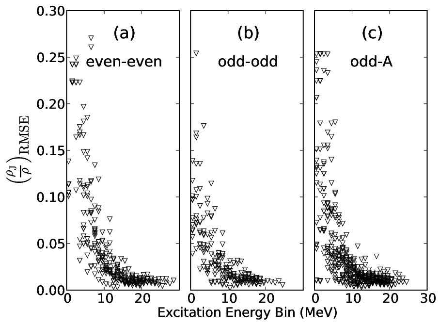
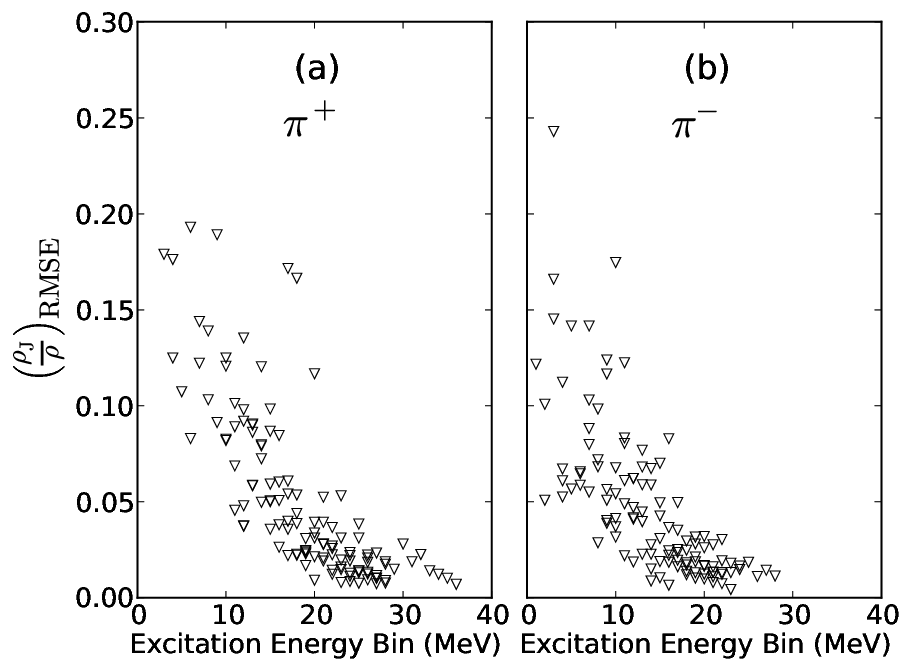
The degree of improvement in appears to be independent of any structural differences in the and shell nuclides, as illustrated in Fig. 7. The cross-shell nuclides in the - space, Fig. 8, exhibit a similar improvement in , though because the levels are split between parities the level density is lower than that of the and shell nuclides, and thus the improvement occurs at higher excitation energies than with the latter.
We also investigated the dependence upon the bin size. While the above results were for standard bin sizes of 1.0 MeV, we also used bins of 0.5 and 2.0 MeV. The best-fit values were insensitive to the bin size, as illustrated in Fig. 9, although the error bars depended upon the bin size, which is primarily an effect of the number of levels in a bin.
We therefore conclude that the spin-cutoff factor is a statistically effective parameterization of the -dependence of the level density, particularly at high energy.
As a final note, there is both experimental [9] and theoretical [13] evidence of an odd-even staggering relative to the Ericson parameterization, i.e. suppression of odd- densities and enhancement of even- densities in even-, even- nuclides. We found no consistent evidence for such odd-even staggering in our calculations, for while some select energy bins did appear to exhibit it (for example as in Fig. 2), neighboring energy bins showed the opposite trend. Our lack of odd-even staggering might be due in part to our modest model space, necessary for full-configuration diagonalization, compared to the larger model spaces used in [13].


IV Monte Carlo calculations
We attained our level densities above through laborious diagonalization of shell-model Hamiltonians, but such calculations are not practical for large model spaces. Therefore we consider other techniques to compute the level density and the spin-cutoff factor, in particular shell-model Monte Carlo (SMMC) [15, 16, 13, 14, 17, 18, 19, 20, 21, 22]. In this section, unlike the previous sections, we use the state density, which includes the degeneracy in , because it arises more naturally for SMMC. The normalized Ericson function for the state density is
| (4) |
Most theoretical calculations of the density of states start from thermodynamics, as the partition function is the Laplace transform of the density of states:
| (5) |
where the trace and the sum are over many-body states and one can interpret as inverse temperature. The density of states itself can be written as . The Laplace transform can be inverted with reasonable reliability through the saddle-point approximation [5], and so now one has the problem of computing the nuclear partition function.
One avenue to compute the many-body partition function is to use auxiliary-field path integrals to evaluate . While such an approach has been successful, it requires a nontrivial amount of computing time; furthermore because one must evaluate the resulting integrals through Monte Carlo sampling, one has to use a well-posed interaction that is free or mostly free of the sign problem [15, 16, 13].
The spin-cutoff factor can be related directly to the average value of in an energy bin. One can either assume the nucleon spins add together randomly [21] or simply replace the discrete Ericson function (4) by a continuous function of and integrate. Then one finds [21, 37]
| (6) |
where indicates an average over the state density, that is,
| (7) |
where refers to a sum over states in an energy bin . Using our densities, we found this approximation worked well, as illustrated in Fig. 10, although our fit tended to be a little higher than the found using (6). If we used the level density rather than the state density we got a better fit, but the state density is natural for SMMC calculations.


The authors of [21] relate the spin-cutoff factor to the moment of inertia by way of the spin response function in imaginary time. In fact, in the SMMC it is straightforward to compute the thermal average of the expectation value of the angular momentum,
| (8) |
This is just the Laplace transform of the sum of in an energy bin, that is if we define the average as
| (9) |
(we deliberately use the notation for the thermal average and for the energy average, to help distinguish the two notationally) then
| (10) |
In the same way one can invert the Laplace transform via the method of steepest descent, one can also extract , or rather, extract and then divide by the level density, as follows. First, find the saddle point, which yields the effective temperature for a given target excitation energy:
| (11) |
For a given effective temperature , the energy is different from that for the saddle point condition for the level density, because of the additional term.
One must also compute the second derivative:
| (12) |
The final result of the method of steepest descent is
| (13) |
The state density itself is computed using the exact same kind of inversion, only without the term in the derivatives. Although we did not carry out any Monte Carlo calculations, we modeled such a calculation by computing several exact and complete spectra, namely 22Na and 33S in the shell and 44Ti in the shell, each of which have dimensions of 4000-7000; from those spectra we constructed the partition function as well as the thermal average of . We then inverted using Eq. (13) and found the average value of in an energy bin is well-reconstructed, as shown in Fig. 11,12. (Note: although in nature one expects the average to increase with excitation energy, with finite model spaces it must turn over at some point, as seen here for 44Ti.)
Although a practical -projection scheme for level densities has been implemented [13], by computing an -projected density and taking , simply computing is significantly computationally cheaper, and appears to be effective in arriving at the spin-cutoff factor.


V Conclusions and acknowledgements
We have carried out a detailed investigation into the spin-cutoff parameterization Eq. (1) of the -dependence of the level density, with particular attention paid to the error bars in the fit to . We confirmed that the spin-cutoff parameterization is a good one, and that as the statistics improve the error bars on decrease. There was no qualitative difference in behavior for different nuclides, and the best fit values were insensitive to bin size.
We also showed that a simple energy average, gives a good value for the spin-cutoff parameter and that one can extract the energy average from a thermal average which one might get naturally out of a quantum Monte Carlo calculation. Such an approach would be computationally more efficient than directly calculating -projected densities, although the latter are achieveable.
The U.S. Department of Energy supported this investigation through grant DE-FG02-96ER40985.
References
- [1] W. Hauser and H. Feshbach, Phys. Rev. 87, 366 (1952).
- [2] T. Rauscher, F.-K. Thielemann, and K.-L. Kratz, Phys. Rev. C 56, 1613 (1997).
- [3] H.A. Bethe, Phys. Rev. 50, 332 (1936).
- [4] A. Gilbert and A.G.W. Cameron, Can. J. Phys. 43, 1446 (1965).
- [5] A. Bohr and B.R. Mottelson, Nuclear Structure vol. 1 (Benjamin, New York, 1969).
- [6] T. Ericson, Adv. Phys. 9, 425 (1960).
- [7] S. M. Grimes, J. D. Anderson, J. W. McClure , B. A. Pohl and C. Wong, Phys. Rev. C 10, 2373 (1974).
- [8] S. M. Grimes, C. H. Poppe, C. Wong, and B. J. Dalton , Phys. Rev. C 18, 1100 (1978)
- [9] T. von Egidy and D. Bucurescu, Phys. Rev. C 78, 051301(R) (2008).
- [10] T. von Egidy and D. Bucurescu, Phys. Rev. C 80, 054310 (2009).
- [11] S. M. Grimes, S. D. Bloom, H. K. Vonach, and R. F. Hausman, Jr. , Phys. Rev. C27, 2893 (1983)
- [12] Po-lin Huang, S. M. Grimes, and T. N. Massey, Phys. Rev C62, 024002(2000).
- [13] Y. Alhassid, S. Liu, and H. Nakada, Phys. Rev. Lett. 99, 162504 (2007).
- [14] K. VanHoucke, S. M. A. Rombouts, K. Heyde, and Y. Alhassid, Phys. Rev. C 79, 024302 (2009).
- [15] G. H. Lang, C. W. Johnson, S. E. Koonin, and W. E. Ormand, Phys. Rev. C 48, 1518 (1993).
- [16] S. E. Koonin, D. J. Dean, and K. Langanke, Phys. Rep. 278, 1 (1997).
- [17] W. E. Ormand, Phys. Rev. C 56, R1678 (1997).
- [18] H. Nakada and Y. Alhassid, Phys Rev. Lett. 79, 2939 (1997).
- [19] H. Nakada and Y. Alhassid, Phys. Lett. B 436, 231 (1998).
- [20] S. Liu and Y. Alhassid, Phys. Rev. Lett. 87, 022501 (2001).
- [21] Y. Alhassid, G. F. Bertsch, L. Fang, and S. Liu, Phys. Rev. C 72, 064326 (2005).
- [22] Y. Alhassid, L. Fang, and H. Nakada, Phys. Rev. Lett. 101, 082501 (2008).
- [23] P.J. Brussard and P.W.M. Glaudemans, Shell-model applications in nuclear spectroscopy (North-Holland Publishing Company, Amsterdam 1977).
- [24] B. A. Brown and B. H. Wildenthal, Annu. Rev. Nucl. Part. Sci. 38, 29 (1988).
- [25] E. Caurier, G. Martínez-Pinedo, F. Nowacki, A. Poves, and A. P. Zuker, Rev. Mod. Phys. 77, 427 (2005).
- [26] B. A. Brown and W. A. Richter, Phys. Rev. C 74, 034315 (2006).
- [27] T. T. S. Kuo and G. E. Brown, Nucl. Phys. A114, 235 (1968).
- [28] A. Poves, J. Sanchez-Solano, E. Caurier, and F. Nowacki, Nucl. Phys. A694, 157 (2001).
- [29] S. Cohen and D. Kurath, Nucl. Phys. 73, 1 (1965).
- [30] B.H. Wildenthal, Prog. Part. Nucl. Phys. 11, 5 (1984).
- [31] D. J. Millener and D. Kurath, Nucl. Phys A 255, 315 (1975).
- [32] C. W. Johnson. W. E. Ormand, and P. G. Krastev, Comp. Phys. Comm. 182, 2235 (2013).
- [33] See Supplmental Material at [URL will be inserted by publisher] for graphs for all nuclides listed in Table 1.
- [34] http://purl.com/net/mpfit
- [35] C. B. Markwardt, Astronomical Data Analysis Software and Systems XVIII, 411, 251 (2009).
- [36] J. Moré, Numerical Analysis 630, 105 ( Springer Berlin Heidelberg, 1978) .
- [37] S. I. Al-Quraishi, S. M. Grimes, T. N. Massey, and D. A. Resler Phys. Rev. C 67, 015803 (2003).