Semi-supervised Eigenvectors for
Large-scale
Locally-biased Learning
Abstract
In many applications, one has side information, e.g., labels that are provided in a semi-supervised manner, about a specific target region of a large data set, and one wants to perform machine learning and data analysis tasks “nearby” that prespecified target region. For example, one might be interested in the clustering structure of a data graph near a prespecified “seed set” of nodes, or one might be interested in finding partitions in an image that are near a prespecified “ground truth” set of pixels. Locally-biased problems of this sort are particularly challenging for popular eigenvector-based machine learning and data analysis tools. At root, the reason is that eigenvectors are inherently global quantities, thus limiting the applicability of eigenvector-based methods in situations where one is interested in very local properties of the data.
In this paper, we address this issue by providing a methodology to construct semi-supervised eigenvectors of a graph Laplacian, and we illustrate how these locally-biased eigenvectors can be used to perform locally-biased machine learning. These semi-supervised eigenvectors capture successively-orthogonalized directions of maximum variance, conditioned on being well-correlated with an input seed set of nodes that is assumed to be provided in a semi-supervised manner. We show that these semi-supervised eigenvectors can be computed quickly as the solution to a system of linear equations; and we also describe several variants of our basic method that have improved scaling properties. We provide several empirical examples demonstrating how these semi-supervised eigenvectors can be used to perform locally-biased learning; and we discuss the relationship between our results and recent machine learning algorithms that use global eigenvectors of the graph Laplacian.
1 Introduction
In many applications, one has information about a specific target region of a large data set, and one wants to perform common machine learning and data analysis tasks “nearby” the pre-specified target region. In such situations, eigenvector-based methods such as those that have been popular in machine learning in recent years tend to have serious difficulties. At root, the reason is that eigenvectors, e.g., of Laplacian matrices of data graphs, are inherently global quantities, and thus they might not be sensitive to very local information. Motivated by this, we consider the problem of finding a set of locally-biased vectors—we will call them semi-supervised eigenvectors—that inherit many of the “nice” properties that the leading nontrivial global eigenvectors of a graph Laplacian have—for example, that capture “slowly varying” modes in the data, that are fairly-efficiently computable, that can be used for common machine learning and data analysis tasks such as kernel-based and semi-supervised learning, etc.—so that we can perform what we will call locally-biased machine learning in a principled manner.
1.1 Locally-biased Learning
By locally-biased machine learning, we mean that we have a data set, e.g., represented as a graph, and that we have information, e.g., given in a semi-supervised manner, that certain “regions” of the data graph are of particular interest. In this case, we may want to focus predominantly on those regions and perform data analysis and machine learning, e.g., classification, clustering, ranking, etc., that is “biased toward” those pre-specified regions. Examples of this include the following.
- •
Locally-biased community identification. In social and information network analysis, one might have a small “seed set” of nodes that belong to a cluster or community of interest [2, 35]; in this case, one might want to perform link or edge prediction, or one might want to “refine” the seed set in order to find other nearby members.
- •
Locally-biased image segmentation. In computer vision, one might have a large corpus of images along with a “ground truth” set of pixels as provided by a face detection algorithm [18, 37, 38]; in this case, one might want to segment entire heads from the background for all the images in the corpus in an automated manner.
- •
Locally-biased neural connectivity analysis. In functional magnetic resonance imaging applications, one might have small sets of neurons that “fire” in response to some external experimental stimulus [42]; in this case, one might want to analyze the subsequent temporal dynamics of stimulation of neurons that are “nearby,” either in terms of connectivity topology or functional response, members of the original set.
In each of these examples, the data are modeled by a graph—which is either “given” from the application domain or is “constructed” from feature vectors obtained from the application domain—and one has information that can be viewed as semi-supervised in the sense that it consists of exogeneously-specified “labels” for the nodes of the graph. In addition, there are typically a relatively-small number of labels and one is interested in obtaining insight about the data graph nearby those labels.
These examples present considerable challenges for standard global spectral techniques and other traditional eigenvector-based methods. (Such eigenvector-based methods have received attention in a wide range of machine learning and data analysis applications in recent years. They have been useful, for example, in non-linear dimensionality reduction [3, 13]; in kernel-based machine learning [53]; in Nyström-based learning methods [65, 58]; spectral partitioning [50, 54, 41], and so on.) At root, the reason is that eigenvectors are inherently global quantities, thus limiting their applicability in situations where one is interested in very local properties of the data. That is, very local information can be “washed out” and essentially invisible to these globally-optimal vectors. For example, a sparse cut in a graph may be poorly correlated with the second eigenvector and thus invisible to a method based only on eigenvector analysis. Similarly, if one has semi-supervised information about a specific target region in the graph, as in the above examples, one might be interested in finding clusters near this prespecified local region in a semi-supervised manner; but this local region might be essentially invisible to a method that uses only global eigenvectors. Finally, one might be interested in using kernel-based methods to find “local correlations” or to regularize with respect to a “local dimensionality” in the data, but this local information might be destroyed in the process of constructing kernels with traditional kernel-based methods.
1.2 Semi-supervised Eigenvectors
In this paper, we provide a methodology to construct what we will call semi-supervised eigenvectors of a graph Laplacian; and we illustrate how these locally-biased eigenvectors (locally-biased in the sense that they will be well-correlated with the input seed set of nodes or that most of their “mass” will be on nodes that are “near” that seed set) inherit many of the properties that make the leading nontrivial global eigenvectors of the graph Laplacian so useful in applications. In order to make this method useful, there should ideally be a “knob” that allows us to interpolate between very local and the usual global eigenvectors, depending on the application at hand; we should be able to use these vectors in common machine learning pipelines to perform common machine learning tasks; and the intuitions that make the leading nontrivial global eigenvectors of the graph Laplacian useful should, to the extent possible, extend to the locally-biased setting. To achieve this, we will formulate an optimization ansatz that is a variant of the usual global spectral graph partitioning optimization problem that includes a natural locality constraint as well as an orthogonality constraint, and we will iteratively solve this problem.
In more detail, assume that we are given as input a (possibly weighted) data graph , an indicator vector of a small “seed set” of nodes, a correlation parameter , and a positive integer . Then, informally, we would like to construct vectors that satisfy the following bicriteria: first, each of these vectors is well-correlated with the input seed set; and second, those vectors describe successively-orthogonalized directions of maximum variance, in a manner analogous to the leading nontrivial global eigenvectors of the graph Laplacian. (We emphasize that the seed set of nodes, the integer , and the correlation parameter are part of the input; and thus they should be thought of as being available in a semi-supervised manner.) Somewhat more formally, our main algorithm, Algorithm 1 in Section 3, returns as output semi-supervised eigenvectors; each of these is the solution to an optimization problem of the form of Generalized LocalSpectral in Figure 1, and thus each “captures” (say) of the correlation with the seed set. Our main theoretical result, described in Section 3, states that these vectors define successively-orthogonalized directions of maximum variance, conditioned on being -well-correlated with an input seed set ; and that each of these semi-supervised eigenvectors can be computed quickly as the solution to a system of linear equations. To extend the practical applicability of this basic result, we will in Section 4 describe several heuristic extensions of our basic framework that will make it easier to apply the method of semi-supervised eigenvectors at larger size scales. These extensions involve using the so-called Nyström method, computing one locally-biased eigenvector and iteratively “peelling off” successive components of interest, as well as performing random walks that are “local” in a stronger sense than our basic method considers.
Finally, in order to illustrate how the method of semi-supervised eigenvectors performs in practice, we also provide a detailed empirical evaluation using a wide range of both small-scale as well as larger-scale data. In particular, we consider two small data sets, one consisting of graphs generated from a popular network generation model and the other data drawn from Congressional roll call voting patterns, in order to illustrate the basic method; we consider graphs constructed from the widely-studied MNIST digit data, in order to illustrate how the method performs on a data set that is widely-known in the machine learning community; and we consider two larger data sets, one consisting of Internet graphs and the other consisting of graphs constructed from fMRI medical imaging, in order to illustrate how the method performs in larger-scale applications.
1.3 Related Work
From a technical perspective, the work most closely related to ours is the recently-developed “local spectral method” of Mahoney et al. [37]. The original algorithm of Mahoney et al. [37] introduced a methodology to construct a locally-biased version of the leading nontrivial eigenvector of a graph Laplacian and also showed (theoretically and empirically in a social network analysis application) that that the resulting vector could be used to partition a graph in a locally-biased manner. From this perspective, our extension incorporates a natural orthogonality constraint that successive vectors need to be orthogonal to previous vectors. Subsequent to the work of [37], [38] applied the algorithm of [37] to to the problem of finding locally-biased cuts in a computer vision application. Similar ideas have also been applied somewhat differently. For example, [2] use locally-biased random walks, e.g., short random walks starting from a small seed set of nodes, to find clusters and communities in graphs arising in Internet advertising applications; [35] used locally-biased random walks to characterize the local and global clustering structure of a wide range of social and information networks; and [29] developed the Spectral Graph Transducer, which performs transductive learning via spectral graph partitioning.
The objectives in both [29] and [37] are constrained eigenvalue problems that can be solved by finding the smallest eigenvalue of an asymmetric generalized eigenvalue problem; but in practice this procedure can be highly unstable [20]. The algorithm of [29] reduces the instabilities by performing all calculations in a subspace spanned by the smallest eigenvectors of the graph Laplacian; whereas the algorithm of [37] performs a binary search, exploiting the monotonic relationship between a control parameter and the corresponding Lagrange multiplier. The form of our optimization problem also has similarities to other work in computer vision applications: e.g., [66] and [18] find good conductance clusters subject to a set of linear constraints.
In parallel, [3] and a large body of subsequent work including [13] used (the usual global) eigenvectors of the graph Laplacian to perform dimensionality reduction and data representation, in unsupervised and semi-supervised settings [59, 51, 67]. Typically, these methods construct some sort of local neighborhood structure around each data point, and they optimize some sort of global objective function to go “from local to global” [52]. In some cases, these methods can be understood in terms of data drawn from an hypothesized manifold [5], and more generally they have proven useful for denoising and learning in semi-supervised settings [4, 6]. These methods are based on spectral graph theory [12]; and thus many of these methods have a natural interpretation in terms of diffusions and kernel-based learning [53, 31, 57, 11, 23]. These interpretations are important for the usefulness of these global eigenvector methods in a wide range of applications. As we will see, many (but not all) of these interpretations can be ported to the “local” setting, an observation that was made previously in a different context [14].
Many of these diffusion-based spectral methods also have a natural interpretation in terms of spectral ranking [61]. “Topic sensitive” and “personalized” versions of these spectral ranking methods have also been studied [26, 28]; and these were the motivation for diffusion-based methods to find locally-biased clusters in large graphs [55, 1, 37]. Our optimization ansatz is a generalization of the linear equation formulation of the PageRank procedure [43, 37, 61]; and its solution involves Laplacian-based linear equation solving, which has been suggested as a primitive is of more general interest in large-scale data analysis [60].
1.4 Outline of the Paper
In the next section, Section 2, we will provide notation and some background and discuss related work. Then, in Section 3 we will present our main algorithm and our main theoretical result justifying the algorithm; and in Section 4 we will present several extensions of our basic method that will help for certain larger-scale applications of the method of semi-supervised eigenvectors. In Section 5, we present an empirical analysis, including both toy data to illustrate how the “knobs” of our method work, as well as applications to realistic machine learning and data analysis problems; and in Section 6 we present a brief discussion and conclustion.
2 Background and Notation
Let be a connected undirected graph with vertices and edges, in which edge has weight For a set of vertices in a graph, the volume of is , in which case the volume of the graph is . In the following, will denote the adjacency matrix of , while will denote the diagonal degree matrix of , i.e., , the weighted degree of vertex . The Laplacian of is defined as . (This is also called the combinatorial Laplacian, in which case the normalized Laplacian of is .)
The Laplacian is the symmetric matrix having quadratic form , for . This implies that is positive semidefinite and that the all-one vector is the eigenvector corresponding to the smallest eigenvalue . The generalized eigenvalues of are . We will use to denote smallest non-trivial eigenvector, i.e., the eigenvector corresponding to ; to denote the next eigenvector; and so on. We will overload notation to use to denote the smallest non-zero generalized eigenvalue of with respect to . Finally, for a matrix let denote its (uniquely defined) Moore-Penrose pseudoinverse. For two vectors , and the degree matrix for a graph , we define the degree-weighted inner product as . In particular, if a vector has unit norm, then . Given a subset of vertices , we denote by the indicator vector of in and by the vector in having all entries set equal to .
3 Optimization Approach to Semi-supervised Eigenvectors
In this section, we provide our main technical results: a motivation and statement of our optimization ansatz; our main algorithm for computing semi-supervised eigenvectors; and an analysis that our algorithm computes solutions of our optimization ansatz.
3.1 Motivation for the Program
Recall the optimization perspective on how one computes the leading nontrivial global eigenvectors of the normalized Laplacian or, equivalently, of the leading nontrivial generalized eigenvectors of . The first nontrivial eigenvector is the solution to the problem GlobalSpectral that is presented on the left of Figure 1. Equivalently, although GlobalSpectral is a non-convex optimization problem, strong duality holds for it and it’s solution may be computed as , the leading nontrivial generalized eigenvector of . (In this case, the value of the objective is , and global spectral partitioning involves then doing a “sweep cut” over this vector and appealing to Cheeger’s inequality.) The next eigenvector is the solution to GlobalSpectral, augmented with the constraint that ; and in general the generalized eigenvector of is the solution to GlobalSpectral, augmented with the constraints that , for . Clearly, this set of constraints and the constraint can be written as , where is a -dimensional all-zeros vector, and where is an orthogonal matrix whose column equals (where , the all-ones vector, is the first column of ).
GlobalSpectral
| minimize | |||
| s.t | |||
LocalSpectral
| minimize | |||
| s.t | |||
Generalized LocalSpectral
| minimize | |||
| s.t | |||
Also presented in Figure 1 is LocalSpectral, which includes a constraint that the solution be well-correlated with an input seed set. This LocalSpectral optimization problem was introduced in [37], where it was shown that the solution to LocalSpectral may be interpreted as a locally-biased version of the second eigenvector of the Laplacian.11 1 In [37], the locality constraint was actually a quadratic constraint, and thus a somewhat involved analysis was required. In retrospect, given the form of the solution, and in light of the discussion below, it is clear that the quadratic part was not “real,” and thus we present this simpler form of LocalSpectral here. This should make the connections with our Generalized LocalSpectral objective more immediate. In particular, although LocalSpectral is not convex, it’s solution can be computed efficiently as the solution to a set of linear equations that generalize the popular Personalized PageRank procedure; in addition, by performing a sweep cut and appealing to a variant of Cheeger’s inequality, this locally-biased eigenvector can be used to perform locally-biased spectral graph partitioning [37].
3.2 Our Main Algorithm
We will formulate the problem of computing semi-supervised vectors in terms of a primitive optimization problem of independent interest. Consider the Generalized LocalSpectral optimization problem, as shown in Figure 1. For this problem, we are given a graph , with associated Laplacian matrix and diagonal degree matrix ; an indicator vector of a small “seed set” of nodes; a correlation parameter ; and an constraint matrix that may be assumed to be an orthogonal matrix. We will assume (without loss of generality) that is properly normalized and orthogonalized so that and . While can be a general unit vector orthogonal to , it may be helpful to think of as the indicator vector of one or more vertices in , corresponding to the target region of the graph.
In words, the problem Generalized LocalSpectral asks us to find a vector that minimizes the variance subject to several constraints: that is unit length; that is orthogonal to the span of ; and that is -well-correlated with the input seed set vector . In our application of Generalized LocalSpectral to the computation of semi-supervised eigenvectors, we will iteratively compute the solution to Generalized LocalSpectral, updating to contain the already-computed semi-supervised eigenvectors. That is, to compute the first semi-supervised eigenvector, we let , i.e., the -dimensional all-ones vector, which is the trivial eigenvector , in which case is an matrix; and to compute each subsequent semi-supervised eigenvector, we let the columns of consist of and the other semi-supervised eigenvectors found in each of the previous iterations.
To show that Generalized LocalSpectral is efficiently-solvable, note that it is a quadratic program with only one quadratic constraint and one linear equality constraint.22 2 Alternatively, note that it is an example of an constrained eigenvalue problem [20]. We thank the numerous individuals who pointed this out to us subsequent to our dissemination of the original version of this paper. In order to remove the equality constraint, which will simplify the problem, let’s change variables by defining the matrix as
That is, is a span for the null space of ; and we will take to be an orthogonal matrix. In particular, this implies that is an Identity and is an Projection. Then, with respect to the variable, Generalized LocalSpectral becomes
| (1) | ||||||
In terms of the variable , the solution to this optimization problem is of the form
| (2) | |||||
for a normalization constant and for some that depends on . The second line follows from the first since is an orthogonal matrix. This so-called “S-proceudre” is described in greater detail in Chapter 5 and Appendix B of [10]. The significance of this is that, although it is a non-convex optimization problem, the Generalized LocalSpectral problem can be solved by solving a linear equation, in the form given in Eqn. (2).
Returning to our problem of computing semi-supervised eigenvectors, recall that, in addition to the input for the Generalized LocalSpectral problem, we need to specify a positive integer that indicates the number of vectors to be computed. In the simplest case, we would assume that we would like the correlation to be “evenly distributed” across all vectors, in which case we will require that each vector is -well-correlated with the input seed set vector ; but this assumption can easily be relaxed, and thus Algorithm 1 is formulated more generally as taking a -dimensional vector of correlation coefficients as input.
To compute the first semi-supervised eigenvector, we will let , the all-ones vector, in which case the first nontrivial semi-supervised eigenvector is
| (3) |
where is chosen to saturate the part of the correlation constraint along the first direction. (Note that the projections from Eqn. (2) are not present in Eqn. (3) since by design .) That is, to find the correct setting of , it suffices to perform a binary search over the possible values of in the interval until the correlation constraint is satisfied, that is, until is sufficiently close to .
To compute subsequent semi-supervised eigenvectors, i.e., at steps if one ultimately wants a total of semi-supervised eigenvectors, then one lets be the matrix of the form
| (4) |
where are successive semi-supervised eigenvectors; and the projection matrix is of the form
due to the the degree-weighted inner norm.
Then, by Eqn. (2), the semi-supervised eigenvector takes the form
In more detail, Algorithm 1 presents pseudo-code for our main algorithm for computing semi-supervised eigenvectors. The algorithm takes as input a graph , a seed set (which could be a general vector , subject for simplicity to the normalization constraints and , but which is most easily thought of as an indicator vector for the local “seed set” of nodes), a number of vectors we want to compute, and a vector of locality parameters , where and (where, in the simplest case, one could choose , , for some ). Several things should be noted about our implementation of our main algorithm. First, as we will discuss in more detail below, we compute the projection matrix only implicitly. Second, a naïve approach to Eqn. (2) does not immediately lead to an efficient solution, since will not be in the span of , thus leading to a large residual. By changing variables so that , the solution becomes
Since is a projection matrix, this expression is equivalent to
| (5) |
Third, regarding the solution , we exploit that is an SPSD matrix, and we apply the conjugate gradient method, rather than computing the explicit pseudoinverse. That is, in the implementation we never explicitly represent the dense matrix , but instead we treat it as an operator and we simply evaluate the result of applying a vector to it on either side. Fourth, we use that can never decrease (here we refer to as the smallest non-zero eigenvalue of the modified matrix), so we only recalculate the upper bound for the binary search when an iteration saturates without satisfying . Estimating the bound is critical for the semi-supervised eigenvectors to be able to interpolate all the way to the global eigenvectors of the graph, so in Section 3.4 we return to a discussion on efficient strategies for computing the leading nontrivial eigenvalue of projected down onto the space perpendicular to the previously computed solutions.
3.3 Discussion of Our Main Algorithm
There is a natural “regularization” interpretation underlying our construction of semi-supervised eigenvectors. To see this, recall that the first step of our algorithm can be computed as the solution of a set of linear equations
| (6) |
for some normalization constant and some that can be determined by a binary search over ; and that subsequent steps compute the analogous quantity, subject to additional constraints that the solution be orthogonal to the previously-computed vectors. The quantity can be interpreted as a “regularized” version of the pseudoinverse of , where serves as the regularization parameter. This interpretation has recently been made precise: [36] show that running a PageRank computation—as well as running other diffusion-based procedures—exactly optimizes a regularized version of the GlobalSpectral (or LocalSpectral, depending on the input seed vector) problem; and [47] provide a precise statistical framework justifying this.
The usual interpretation of PageRank involves “random walkers” who uniformly (or non-uniformly, in the case of Personalized PageRank) “teleport” with a probability . As described in [37], choosing corresponds to choosing . By rearranging Eqn. (6) as
we recognize as the standard random walk matrix, and it becomes immediate that the solution based on random walkers,
is divergent for . Since corresponds to no regularization and corresponds to heavy regularization, viewing this problem in terms of solving a linear equation is formally more powerful than viewing it in terms of random walkers. That is, while all possible values of the regularization parameter—and in particular the (positive) value —are achievable algorithmically by solving a linear equation, only values in are achievable by running a PageRank diffusion. In particular, if the optimal value of that saturates the -dependent locality constraint is negative, then running the PageRank diffusion could find it; otherwise, the “best” one could do will still not saturate the locality constraint, in which case some of the intended correlation is “unused.”
An important technical and practical point has to do with the precise manner in which the vector is well-correlated with the seed set . In our formulation, this is captured by a locality parameter that is chosen (via a binary search) to “saturate” the correlation condition, i.e., so that the vector is -well-correlated with the input seed set. As a general rule, successive s need to be chosen that successive vectors are less well-localized around the input seed set. (Alternatively, depending on the application, one could choose this parameter so that successive s are equal; but this will involve “sacrificing” some amount of the correlation, which will lead to the last or last few eigenvectors being very poorly-correlated with the input seed set. These tradeoffs will be described in more detail below.) Informally, if is a seed set consisting of a small number of nodes that are “nearby” each other, then to maintain a given amount of correlation, we must “view” the graph over larger and larger size scales as we compute more and more semi-supervised eigenvectors. More formally, we need to let the value of the regularization parameter at the round, we call it , vary for each . That is, is not pre-specified, but it is chosen via a binary search over the region , where is the leading nontrivial eigenvalue of projected down onto the space perpendicular to the previously-computed vectors (which is in general larger than ). In this sense, our semi-supervised eigenvectors are both “locally-biased”, in a manner that depends on the input seed vector and correlation parameter, and “regularized”, in a manner that depends on the local graph structure.
To illustrate the previous discussion, Figure 2 considers the two-dimensional grid. In each subfigure, the blue curve shows the correlation with a single seed node as a function of for the leading semi-supervised eigenvector, and the black dot illustrates the value of for three different values of the locality parameter . This relationship between and is in general non-convex, but it is monotonic for . The red curve in each subfigure shows the decay for the second semi-supervised eigenvector. Recall that it is perpendicular to the first semi-supervised eigenvector, that the decay is monotonic for , and that . In Figure 2(a), the first semi-supervised eigenvector is not “too” close to , and so (i.e., the second eigenvalue of the next semi-supervised eigenvector) increases just slightly. In Figure 2(b), we consider a locality parameter that leads to a value of that is closer to , thereby increasing the value of . Finally, in Figure 2(c), the locality parameter is such that the leading semi-supervised eigenvector almost coincides with ; this results in , as required if we were to compute the global eigenvectors.
3.4 Bounding the Binary Search
For the following derivations it is more convenient to consider the normalized graph Laplacian, in which case we define the first solution as
| (7) |
where . This approach is convenient since the projection operator with null space defined by previous solutions can be expressed as , assuming that . That is, is of the form
where are successive solutions to Eqn. (7). In the following the type of projection operator will be implicit from the context, i.e., when working with the combinatorial graph Laplacian , whereas for the normalized graph Laplacian .
For the normalized graph Laplacian , the eigenvalues of equal the eigenvalues of the generalized eigenvalue problem . The binary search employed in Algorithm 1 uses a monotonic relationship between the parameter and the correlation with the seed , that can be deduced from the KKT-conditions [37]. Note, that if the upper bound for the binary search is not determined with sufficient precision, the search will (if we underestimate ) fail to satisfy the constraint, or (if we overestimate ) fail to converge because the monotonic relationship no longer hold.
By Lemma 1 in Appendix A it follows that when . Since the latter term is a sum of two PSD matrices, the value of the upper bound can only increase as stated by Lemma 2 in Appendix A. This is an important property, because if we do not recalculate , the previous value is guaranteed to be an underestimate, meaning that the objective will remain convex. Thus, it may be more efficient to first recompute when the binary search fails to satisfy , meaning that must be recomputed to increase the search range.
We compute the value for the upper bound of the binary search by transforming the problem in such a way that we can determine the greatest eigenvalue of a new system (fast and robust), and from that, deduce the new value of . We do so by expanding the expression as
Since all columns of will be eigenvectors of with zero eigenvalue, these will all be eigenvectors of with eigenvalue . Hence, the largest algebraic eigenvalue can be used to compute the upper bound for the binary search as
| (8) |
The reason for not considering the largest magnitude eigenvalue, is that may be indefinite. Finally, with respect to our implementation we emphasize that is used as a projection operator, and not represented explicitly.
4 Extension of Our Main Algorithm and Implementation Details
In this section, we present two variants of our main algorithm that are more well-suited for very large-scale applications; the first uses a column-based low-rank approximation, and the second uses random walk ideas. In Section 4.1, we describe how to use the Nyström method, which constructs a low-rank approximation to the kernel matrix by sampling columns, to construct a general solution for semi-supervised eigenvectors, where the low-rankness is exploited for very efficient computation. Then, in Section 4.2, we describe a “Push-peeling heuristic,” based on the efficient Push algorithm by [1]. The basic idea is that if, rather than iteratively computing locally-biased semi-supervised eigenvectors using the procedure described in Algorithm 1, we instead compute solutions to LocalSpectral and then construct the semi-supervised eigenvectors by “projecting away” pieces of these solutions, then we can take advantage of local random walks that have improved algorithmic properties.
4.1 A Nyström-based Low-rank Approach
Here we describe the use of the recently-popular Nyström method to speed up the computation of semi-supervised eigenvectors. We do so by considering how a low-rank decomposition can be exploited to yield solutions to the Generalized LocalSpectral objective in Figure 1, where the running time largely depends on a matrix-vector product. These methods are most appropriate when the kernel matrix is reasonably well-approximated by a low-rank matrix [15, 22, 64].
Given some low-rank approximation , we apply the Woodbury matrix identity, and we derive an explicit solution for the leading semi-supervised eigenvector
where . In order to compute efficiently the subsequent semi-supervised eigenvectors we must accommodate for the projection operator , while yet exploiting the explicit closed-form inverse . However, the projection operator complicates the expression, since the previous solution can be spanned by multiple global eigenvectors, so leveraging from the low-rank decomposition is more difficult for the inverse .
Conveniently, we can decouple the projection operator by treating the orthogonality constraint using a Lagrangian approach, such that the solution can be expressed as
where denotes the associated Lagrange multiplier, and where the sign is deduced from the KKT conditions. Applying the Woodbury matrix identity is now straightforward
| where for notational convenience we have introduced . By decomposing with an eigendecomposition the equation simplifies as follows | ||||
| where . Note how this result gives a well defined way of controlling the amount of “orthogonality”, and by Lemma 1 in Appendix A, we get exact orthogonality in the limit of , in which case the expression simplifies to | ||||
| Using the explicit expression for , the solution now only involves matrix-vector products and the inverse of a small matrix | ||||
| (9) | ||||
To conclude this section, let us also consider how we can optimize the efficiency of the calculation of used for bounding the binary search in Algorithm 1. According to Eqn. (8) the bound can be calculated efficiently as . However, by substituting with , we can exploit low-rankness since
where the latter is a much smaller system.
4.2 A Push-peeling Heuristic
Here we present a variant of our main algorithm that exploits the connections between diffusion-based procedures and eigenvectors, allowing semi-supervised eigenvectors to be efficiently computed for large networks. This is most well-known for the leading nontrivial eigenvectors of the graph Laplacian [12]; but recent work has exploited these connections in the context of performing locally-biased spectral graph partitioning [55, 1, 37]. In particular, we can compute the locally-biased vector using the first step of Algorithm 1, or alternatively we can compute it using a locally-biased random walk of the form used in [55, 1]. Here we present a heuristic that works by peeling off components from a solution to the PageRank problem, and by exploiting the regularization interpretation of , we can from these components obtain the subsequent semi-supervised eigenvectors.
Specifically, we focus on the Push algorithm by [1]. This algorithm approximates the solution to PageRank very efficiently, by exploiting the local modifications that occur when the seed is highly concentrated. This makes our algorithm very scalable and applicable for large-scale data, since only the local neighborhood near the seed set will be touched by the algorithm. In comparison, by solving the linear system of equations we explicitly touch all nodes in the graph, even though most spectral rankings will be below the computational precision [8].
We adapt a similar notation as in [1] and start by defining the usual PageRank vector as the unique solution of the linear system
| (10) | ||||
| where is the teleportation parameter, and is the sparse starting vector. For comparison, the push algorithm by [1] computes an approximate PageRank vector for a slightly different system | ||||
where and not the usual random walk matrix as used in Eqn. (10). However, these equations are only superficially different, and equivalent up to a change of the respective teleportation parameter. Thus, it is straightforward to verify that these teleportation parameters and the parameter of Eqn. (6) are related as
and that the leading semi-supervised eigenvector for can be approximated as
To generalize subsequent semi-supervised eigenvectors to this diffusion based framework, we need to accommodate for the projection operator such that subsequent solutions can be expressed in terms of graph diffusions. By requiring distinct values of for all semi-supervised eigenvectors, we may use the solution for the leading semi-supervised eigenvector and then systematically “peel off” components, thereby obtaining the solution of one of the consecutive semi-supervised eigenvectors. By Lemma 5, in Appendix A the general solution in Eqn. (5) can be approximated by
| (11) |
under the assumption that all for are sufficiently apart. If we think about as being distinct eigenvalues of the generalized eigenvalue problem , then it is clear that Eqn. (11), correctly computes the sequence of generalized eigenvectors. This is explained by the fact that can be interpreted as the first step of the Rayleigh quotient iteration, where is the estimate of the eigenvalue, and is the estimate of the eigenvector. Given that the estimate of the eigenvalue is right, this algorithm will in the initial step compute the corresponding eigenvector, and the operator will be superfluous, as the global eigenvectors are already orthogonal in the degree-weighted norm. To quantify the failure modes of the approximation, let us consider what happens when starts to approach . What constitutes the second solution for a particular value of is the perpendicular component with respect to the projection onto the solution given by . As approaches , this perpendicular part diminishes and the solution becomes ill-posed. Fortunately, we can easily detect such issues during the binary search in Algorithm 1, and in general the approximation has turned out to work very well in practice as our experimental results in Section 5 show.
In terms of the approximate PageRank vector , the general approximate solution takes the following form
| (12) |
As already stated in Section 3.3, the impact of using a diffusion based procedure is that we cannot interpolate all the way to the global eigenvectors, and that the main challenge is that the solutions do not become too localized. The parameter of the Push algorithm controls the threshold for propagating mass away from the seed set and into the adjacent nodes in the graph. If the threshold is too high, the solution will be very localized and make it difficult to find more than a few semi-supervised eigenvectors, as characterized by Lemma 3 in Appendix A, because the leading ones will then span the entire space of the seed set. As the choice of is important for the applicability of our algorithm, we will in Section 5 investigate the influence of this parameter on large data graphs.
To conclude this section, we consider an important implementation detail that have been omitted so far. In the work of [37] the seed vector was defined to be perpendicular to the all-ones vector, and for the sake of consistency we have chosen to define it in the same way. The impact of projecting the seed set to a space that is perpendicular to the all-ones vector is that the resulting seed vector is no longer sparse, making the use of the Push algorithm in Eqn. (12) inefficient. The seed vector can, however, without loss of generality, be defined as where is the sparse seed, and is the leading eigenvector of the normalized graph Laplacian (corresponding to the all-ones vector of the combinatorial graph Laplacian). If we substitute with this expression for the seed in Eqn. (12), it follows by plain algebra (see Appendix B) that
| (13) |
Now the Push algorithm is only defined on the sparse seed set making the the expression very scalable. Finally, the Push algorithm maintains a queue of high residual nodes that are yet to be processed. The order in which nodes are processed influences the overall running time, and in [8] preliminary experiments showed that a FIFO queue resulted in the best performance for large values of , as compared to a priority queue that scales logarithmically. For this reason we have chosen to use a FIFO queue in our implementation.
5 Empirical Results
In this section, we provide a detailed empirical evaluation of the method of semi-supervised eigenvectors and how it can be used for locally-biased machine learning. Our goal is two-fold: first, to illustrate how the “knobs” of the method work; and second, to illustrate the usefulness of the method in real applications. To do this, we consider several classes of data.
- •
Toy data. In Section 5.1, we consider one-dimensional examples of the popular “small world” model [62]. This is a parameterized family of models that interpolates between low-dimensional grids and random graphs; and, as such, it allows us to illustrate the behavior of the method and its various parameters in a controlled setting.
- •
Congressional voting data. In Section 5.2, we consider roll call voting data from the United States Congress that are based on [49]. This is an example of realistic data set that has relatively-simple global structure but nontrivial local structure that varies with time [14]; and thus it allows us to illustrate the method in a realistic but relatively-clean setting.
- •
Handwritten image data. In Section 5.3, we consider data from the MNIST digit data set [34]. These data have been widely-studied in machine learning and related areas and they have substantial “local heterogeneity.” Thus, these data allow us to illustrate how the method may be used to perform locally-biased versions of common machine learning tasks such as smoothing, clustering, and kernel construction.
- •
Functional brain imaging data. In Section 5.4, we consider functional magnetic resonance imaging (fMRI) data. Single subject fMRI data is characterized by high dimensionality and relatively few samples, in contrast to the MNIST data that consist of many samples and a relatively low dimensionality. We demonstrate how our semi-supervised eigenvectors can be applied to construct a data-driven spatially-biased basis by incorporating a priori knowledge from a functional brain atlas [17].
- •
Large-scale network data. In Section 5.5, we consider large-scale network data, and demonstrate significant performance improvements of the push-peeling heuristic compared to solving the same equations using a conjugate gradient solver. These improvements are demonstrated on datasets from the DIMACS implementation challenge, as well as on large web-crawls with more then 3 billion non-zeros in the adjacency matrix [44, 45, 46].
5.1 Small-world Data
The first data sets we consider are networks constructed from the so-called small-world model. This model can be used to demonstrate how semi-supervised eigenvectors focus on specific target regions of a large data graph to capture slowest modes of local variation; and it can also be used to illustrate how the “knobs” of the method work, e.g., how and interplay, in a practical setting. In Figure 3, we plot the usual global eigenvectors, as well as locally-biased semi-supervised eigenvectors, around illustrations of non-rewired and rewired realizations of the small-world graph, i.e., for different values of the rewiring probability and for different values of the locality parameter .
,
,
,
,
.

,
,
,
,
.

, ,
,
,
,
.

, ,
,
,
,
.

To start, in Figure 3(a) that we show a graph with no randomly-rewired edges () and a parameter such that the global eigenvectors are obtained. This yields a symmetric graph with eigenvectors corresponding to orthogonal sinusoids, i.e., the first two capture the slowest mode of variation and correspond to a sine and cosine with equal random phase-shift (up to a rotational ambiguity). In Figure 3(b), random edges have been added with probability and the parameter is still chosen such that the global eigenvectors—now of the rewired graph—are obtained. Note the many small kinks in the eigenvectors at the location of the randomly added edges. Note also the slow mode of variation in the interval on the top left; a normalized-cut based on the leading global eigenvector would extract this region, since the remainder of the ring is more well-connected due to the random rewiring.
In Figure 3(c), we see the same graph realization as in Figure 3(b), except that the semi-supervised eigenvectors have a seed node at the top of the circle, i.e., at “12 o-clock,” and the locality parameter , which corresponds to moderately well-localized eigenvectors. As with the global eigenvectors, the locally-biased semi-supervised eigenvectors are of successively-increasing (but still localized) variation. Note also that the neighborhood around “11 o-clock” contains more mass, e.g., when compared with the same parts of the circle in Figure 3(b) or with other parts of the circle in Figure 3(c), even though it is not very near the seed node in the original graph geometry. The reason for this is that this region is well-connected with the seed via a randomly added edge, and thus it is close in the modified graph topology. Above this visualization, we also show the value of that saturates , i.e., is the Lagrange multiplier that defines the effective locality . Not shown is that if we kept reducing , then would tend towards , and the respective semi-supervised eigenvectors would tend towards the global eigenvectors that are illustrated in Figure 3(b). Finally, in Figure 3(d), the desired locality is increased to (which has the effect of decreasing the value of ), making the semi-supervised eigenvectors more localized in the neighborhood of the seed. It should be clear that, in addition to being determined by the locality parameter, we can think of as a regularizer biasing the global eigenvectors towards the region near the seed set. That is, variation in eigenvectors that are near the initial seed (in the modified graph topology) are most important, while variation that is far away from the initial seed matters much less.
5.2 Congressional Voting Data
The next data set we consider is a network constructed from a time series of roll call voting patterns from the United States Congress that are based on [49]. This is a particularly well-structured social network for which there is a great deal of meta-information, and it has been studied recently with graph-based methods [40, 63, 14]. Thus, it permits a good illustration of the method of semi-supervised eigenvectors in a real application [48]. This data set is known to have nontrivial time-varying structure at different time steps, and we will illustrate how the method of semi-supervised eigenvectors can perform locally-biased classification with a traditional kernel-based algorithm.
In more detail, we evaluate our method by considering the known Congress data-set containing the roll call voting patterns in the U.S Senate across time. We considered Senates in the Congress through the Congress, thus covering the years to . During this time, the U.S went from to states, hence the number of senators in each of these Congresses was roughly the same. We constructed an adjacency matrix, with ( Congresses each with Senators) where represents the extent of voting agreement between legislators and , and where identical senators in adjacent Congresses are connected with an inter-Congress connection strength. We then considered the Laplacian matrix of this graph, constructed in the usual way [14].

Figure 4 visualizes the adjacency matrix, along with four of the individual Congresses, color coded by party. This illustrates that these data should be viewed—informally—as a structure (depending on the specific voting patterns of each Congress) evolving along a one-dimensional temporal axis, confirming the results of [14]. Note that the latter two Congresses are significantly better described by a simple two-clustering than the former two Congresses, and an examination of the clustering properties of each of the Congresses reveals significant variation in the local structure of individual Congresses, in a manner broadly consistent with [48] and [49]. In particular, the more recent Congresses are significantly more polarized.
The first vertical column of Figure 5 illustrates the first three global eigenvectors of the full data set, illustrating fluctuations that are sinusoidal and consistent with the one-dimensional temporal scaffolding. Also shown in the first column are the values of that eigenfunction for the members of the Congress, illustrating that there is not a good separation based on party affiliations. The next three vertical columns of Figure 5 illustrate various localized eigenvectors computed by starting with a seed node in the Congress. For the second column, we visualize the semi-supervised eigenvectors for a very low correlation (), which corresponds to only a weak localization—in this case one sees eigenvectors that look very similar to the global eigenvectors, and the elements of the eigenvector on that Congress do not reveal partitions based on the party cuts.
The third and fourth column of Figure 5 illustrate the semi-supervised eigenvectors for a much higher correlation (), meaning a much stronger amount of locality. In particular, the third column starts with the seed node marked in Figure 4, which is at the articulation point between the two parties, while the fourth column starts with the seed node marked , which is located well within the cluster of Republicans. In both cases the eigenvectors are much more strongly localized on the Congress near the seed node, and in both cases one observes the partition into two parties based on the elements of the localized eigenvectors. Note, however, that when the initial seed is at the articulation point between two parties then the situation is much noisier: in this case, this “partitionability” is seen only on the third semi-supervised eigenvector, while when the initial seed is well within one party then this is seen on all three eigenvectors. Intuitively, when the seed set is strongly within a good cluster, then that cluster tends to be found with semi-supervised eigenvectors (and we will observe this again below). This is consistent with the diffusion interpretation of eigenvectors. This is also consistent with [14], who observed that the properties of eigenvector localization depended on the local structure of the data around the seed node, as well as the larger scale structure around that local cluster.
To illustrate how these structural properties manifest themselves in a more traditional machine learning task, we also consider the classification task of discriminating between Democrats and Republicans in single Congresses, i.e., we measure to what extent we can extract local discriminative features. To do so, we apply -regularized -loss support vector classification with a linear kernel, where features are extracted using the global eigenvectors of the entire data set, global eigenvectors from a single Congress (best case measure), and our semi-supervised eigenvectors. Figure 6 illustrates the classification accuracy for , , and eigenvectors. As reported by [14], locations that exhibit discriminative information are best found on low-order eigenvectors of this data, explaining why the classifier based global eigenvectors performs poorly. In the classifier based on global eigenvectors in the single Congress we exploit a priori knowledge to extract the relevant data, that in a usual situation would be impossible. Hence, this is simply to define a baseline point of reference for the best case classification accuracy. The classifier based on semi-supervised eigenvectors is seeded using a few training samples and performs in-between the two other approaches. Compared to our point of reference, Congresses in the range to do worse with the semi-supervised eigenvectors; whereas for Congresses after the semi-supervised approach almost performs on par, even for a single single eigenvector. This is consistent with the visualization in Figure 4 illustrating that earlier Congresses are less cleanly separable, as well as with empirical evidence indicating heterogeneity due to Southern Democrats in earlier Congresses and the recent increase in party polarization in more recent Congresses, as described in [48] and [49].
5.3 MNIST Digit Data
The next data set we consider is the well-studied MNIST data set containing training digits and test digits ranging from to ; and, with these data, we demonstrate the use of semi-supervised eigenvectors as a feature extraction preprocessing step in a traditional machine learning setting. We construct the full -NN graph, with and with edge weights given by , where is the Euclidian distance of the node to it’s nearest neighbor; and from this we define the graph Laplacian in the usual way. We then evaluate the semi-supervised eigenvectors in a transductive learning setting by disregarding the majority of labels in the entire training data. We use a few samples from each class to seed our semi-supervised eigenvectors as well as a few others to train a downstream classification algorithm. For this evaluation, we use the Spectral Graph Transducer (SGT) of [29]; and we choose to use it for two main reasons. First, the transductive classifier is inherently designed to work on a subset of global eigenvectors of the graph Laplacian, making it ideal for validating that the localized basis constructed by the semi-supervised eigenvectors can be more informative when we are solely interested in the “local heterogeneity” near a seed set. Second, using the SGT based on global eigenvectors is a good point of comparison, because we are only interested in the effect of our subspace representation. (If we used one type of classifier in the local setting, and another in the global, the classification accuracy that we measure would obviously be confounded.) As in [29], we normalize the spectrum of both global and semi-supervised eigenvectors by replacing the eigenvalues with some monotonically increasing function. We use , i.e., focusing on ranking among smallest cuts; see [11]. Furthermore, we fix the regularization parameter of the SGT to , and for simplicity we fix for all semi-supervised eigenvectors, implicitly defining the effective . Clearly, other correlation distributions and other values of parameter may yield subspaces with even better discriminative properties (which is an issue to which we will return in Section 5.3.2 in greater detail).
| #Semi-supervised eigenvectors for SGT | #Global eigenvectors for SGT | ||||||||||||
| Labeled points | 1 | 2 | 4 | 6 | 8 | 10 | 1 | 5 | 10 | 15 | 20 | 25 | |
| 0.39 | 0.39 | 0.38 | 0.38 | 0.38 | 0.36 | 0.50 | 0.48 | 0.36 | 0.27 | 0.27 | 0.19 | ||
| 0.30 | 0.31 | 0.25 | 0.23 | 0.19 | 0.15 | 0.49 | 0.36 | 0.09 | 0.08 | 0.06 | 0.06 | ||
| 0.12 | 0.15 | 0.09 | 0.08 | 0.07 | 0.06 | 0.49 | 0.09 | 0.08 | 0.07 | 0.05 | 0.04 | ||
| 0.09 | 0.10 | 0.07 | 0.06 | 0.05 | 0.05 | 0.49 | 0.08 | 0.07 | 0.06 | 0.04 | 0.04 | ||
| 0.03 | 0.03 | 0.03 | 0.03 | 0.03 | 0.03 | 0.49 | 0.10 | 0.07 | 0.06 | 0.04 | 0.04 | ||
5.3.1 Discriminating between pairs of digits
Here, we consider the task of discriminating between two digits; and, in order to address a particularly challenging task, we work with s and s. (This is particularly challenging since these two classes tend to overlap more than other combinations since, e.g., a closed can resemble a more than an open .) Hence, we expect that the class separation axis will not be evident in the leading global eigenvector, but instead it will be “buried” further down the spectrum; and we hope to find a “locally-biased class separation axis” with locally-biased semi-supervised eigenvectors. Thus, this example will illustrate how semi-supervised eigenvectors can represent relevant heterogeneities in a local subspace of low dimensionality. See Table 1, which summarizes our classification results based on, respectively, semi-supervised eigenvectors and global eigenvectors, when we use the SGT. See also Figure 7 and Figure 8, which illustrate two realizations for the 1:10 configuration. In these two figures, the training samples are fixed; and, to demonstrate the influence of the seed, we have varied the seed nodes. In particular, in Figure 7 the seed nodes and are located well-within the respective classes; while in Figure 8, they are located much closer to the boudary between the two classes. As intuitively expected, when the seed nodes fall well within the classes to be differentiated, the classification is much better than when the seed nodes are located closer to the boundary between the two classes. See the caption in these figures for further details.


5.3.2 Effect of choosing the correlation/locality parameter
Here, we discuss the effect of the choice of the correlation/locality parameter at different steps of Algorithm 1, e.g., how should be distributed among the components. For example, will the downstream classifier benefit the most from a uniform distribution or will there exist some other nonuniform distribution that is better? Although this will be highly problem specific, one might hope that in realistic applications the classification performance is not too sensitive to the actual choice of distribution. To investigate the effect in our example of discriminating between s and s, we consider semi-supervised eigenvectors for various distributions. Our results are summarized in Figure 9.
Figures 9(a), 9(b), and 9(c) show, for the global eigenvectors and for semi-supervised eigenvectors, where the vector has been chosed to be very nonuniform and very uniform, the top three (global or semi-supervised) eigenvectors plotted against each other as well as the ROC curve for the SGT classifier discriminating between s and s; and Figure 9(d) shows the test error as the vector is varied over the unit simplex. In more detail, red (respectively, blue) corresponds to s (respectively, s), and green points are the remaining digits; and, for Figures 9(b) and 9(c), the semi-supervised eigenvectors are seeded using 50 samples from each target class (s vs. s) and having a non-uniform distribution of , as specified. As seen from the visualization of the semi-supervised eigenvectors in Figures 9(b) and 9(c), the classes are much better separated than by using the global eigenvectors, which are shown in Figure 9(a). For example, this is supported by the Area Under the Curve (AUC) and Error Rate (ERR), being the point on the Receiver Operating Characteristic (ROC) curve that corresponds to having an equal probability of miss-classifying a positive or negative sample, which is a fair estimate as the classes in the MNIST data set is fairly balanced. For Figure 9(c), where we use a uniform distribution of , the classifier performs slightly better than in Figure 9(b), which uses the non-uniform distribution (but both semi-supervised approaches are significantly better than the using the global eigenvectors). For Figure 9(d), we see the test error on the simplex defined by . To obtain this plot we sampled 500 different distributions according to a uniform Dirichlet distribution. With the exception of one extreme very nonuiform corner, the classification accuracy is not too sensitive to the choice of distribution. Thus, if we think of the semi-supervised eigenvectors as a locally-regularized version of the global eigenvectors, the desired discriminative properties are not too sensitive to the details of the locally-biased regularization.


5.3.3 Effect of approximately computing semi-supervised eigenvectors
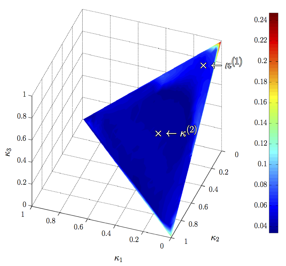
Here, we discuss of the push-peeling procedure from Section 4 that is designed to compute efficient approximations to the semi-supervised eigenvectors by using local random walks to compute an approximation to personalized PageRank vectors. Consider Figure 10, which shows results for two values of the parameter (i.e., the parameter in the push algorithm that implicitly determines how many nodes will be touched). Again we construct the full -NN graph, with and with edge weights given by , where is the Euclidian distance of the node to it’s nearest neighbor; and from this we define the graph Laplacian in the usual way. Using this representation we compute semi-supervised eigenvectors seeding using 50 samples from each class (s vs. s). However, in this case, we fix the regularization parameter vector as ; and note that choosing these specific values correspond to the solutions visualized in Figure 9(c) when the equations are solved exactly. Figure 10(a) shows the results for . This approximation gives us sparse solutions, and the histogram in the second row illustrates the digits that are assigned a nonzero value in the respective semi-supervised eigenvector. In particular, note that most of the mass of the eigenvector is distributed on s and s; but, for this choose of , only few digits of interest (, meaning, in particular, that not all of the s and s) have been touched by the algorithm. This results in the lack of a clean separation between the two classes as one sweeps along the leading semi-supervised eigenvector, as illustrated in the first row; the very uniform correlation distribution ; and the high classification error, as shown in the ROC curve in the bottom panel.
Consider, next, Figure 10(b), which shows the results for , i.e., where the locality parameter has been reduced by an order of magnitude. In this case, the algorithm reproduces the solution by touching only of the nodes in the graph, i.e., basically all of the s and s and only a few other digits. This leads to a much cleaner separation between the two classes as one sweeps over the leading semi-supervised eigenvector; a much more uniform distribution over ; and a classification accuracy that is much better and is similar to what we saw in Figure 9(c). This example illustrates that this push-peeling approximation provides a principled manner to generalize the concept of semi-supervised eigenvectors to large-scale settings, where it will be infeasible to touch all nodes of the graph.
Test data sorted along .
Touched of nodes.

Test data sorted along .
Touched of nodes.

5.3.4 Effect of low-rank Nyström approximation
Here we discuss the use of the low-rank Nyström approximation which is commonly used in large-scale kernel-based machine learning. The memory requirements for representing the explicit kernel matrix, that we here take to be our graph, scales with , whereas inverting the matrix scales with , which, in large-scale settings, is infeasible. The Nyström technique subsamples the dataset to approximate the kernel matrix, and the memory requirements scales with and runs in , where is size of the subsample. For completeness we include the derivation of the Nyström approximation for the normalized graph Laplacian in Appendix C.
In the beginning of Section 5.3 we constructed the -nearest neighbor graph, with and with edge weights given by . Such a sparse construction reduces the effect of “hubs”, as well as being fairly insensitive to the choice of kernel parameter, as the 10 nearest neighbors are likely to be very close in the Euclidian norm. Because the Nyström method will approximate the dense kernel matrix, the choice of kernel parameter is more important, so in the following we will consider the interplay between this parameter, as well as the rank parameter of the Nyström approximation. Moreover, to allow us to compare a rank- Nyström approximation with the full rank- kernel matrix, we choose to subsample the dataset for all of the following experiments, due to the memory requirements. Thus, to provide a baseline, Figure 11 shows results based on a -nearest neighbor graph constructed from and percent of the training data, where in both cases we used for the test data. For both cases, when compared with the results of Figure 9(c), the classification quality is degraded, and so we emphasize that the goal of the following results are not to outperform the results reported in Figure 9(c), but to be comparable with this baseline.


In light of this baseline, Figure 12 provides a thorough analysis for the choices of that we used. Figures 12(a) and 12(b) show the classification error when using the global eigenvectors, for various rank approximations based on the Nyström method as well as the exact method (corresponding to ). Interestingly, these two plots are very dissimilar in terms of their behavior as a function of the number of components. In particular, the plot in Figure 12(b) shows that the low rank approximations for a given set of components outperform the high rank approximations, and the exact representation fails to reduce the error beyond for any of the considered set of components. This may seem counterintuitive, but the reason for this type of behavior is that the relevant global eigenvectors, for , are located far from the end of the spectrum (if we visualized more components for the classification error would eventually drop). For the same reason, the low rank approximations improve more rapidly than the high rank approximations, as the latter approximate the lower part of the spectrum better, and these turn out to have poor discriminative properties. In contrast, the results shown in Figure 12(a) provide good class separation in the lower part of the spectrum, resulting in the high rank approximations to reduce the error most rapidly.
Finally, Figures 12(c) and 12(d) show the classification error for the SGT trained using the semi-supervised eigenvectors. (Note that the scale of the x-axis is much smaller in these subfigures.) For both kernel widths (in both Figures 12(c) and 12(d)), the ordering of the approximations are similar, i.e., the semi-supervised eigenvectors constructed from the approximation performs the best. Moreover, the gap between the and is largest for , again suggesting this approximation is of insufficient rank to model the relevant local heterogeneities deep down in the spectrum; whereas for , the the approximation comes very close to the exact representation, suggesting that local structures are well modeled near the end of the spectrum.
To summarize these results, the method of semi-supervised eigenvectors successfully extracts relevant local structures to perform locally-biased classification, even when they are located far from the end of the spectrum. Moreover, in both cases we considered, the classification error is reduced significantly by using only a few locally-biased components. This contrasts with the global eigenvectors, where for at least eigenvectors are needed in order to obtain similar performance; and for , the classification error remains high even for eigenvectors in case of .
5.3.5 Implementation issues and running time considerations
Here, we discuss implementation details and investigate the advantage of using the Graphics Processing Unit (GPU) for computing semi-supervised eigenvectors. Although the computations underlying the construction of semi-supervised eigenvectors could be performed in many computational environments, the GPU architecture fits well with the dense semi-supervised eigenvector computation in Eqn. (9); for each component, this expression will be executed times within the binary search of Algorithm 1.
Compared to a Central Processing Unit (CPU), which is well-suited for processing code with a complex control flow, a GPU is much better suited for addressing problems that can be expressed as data-parallel computations with a high arithmetic intensity [33, 9, 25]. A GPU consists of a set of Multi Processors (MPs), each containing multiple Scalar Processors (SPs), as well as different types of local memories that the SPs may access. All MPs have also access to a large global memory that, compared to their internal memories, is much slower to access. A computation task to be executed on such a device is usually setup in a grid, where each element in the grid gets assigned to a thread. The grid is then decomposed into blocks that are scheduled onto the MPs with available resources, and the assigned MP will schedule the elements of the block onto its SPs in warps with 32 threads. The best performance is obtained when all threads in a warp execute the same instruction and when the total number of threads in the grid is large, as this allows various latencies to be overlapped with arithmetic operations.
We compare most recent CPU and GPU devices in computing the solution to Eqn. (9). In terms of the GPUs we test both consumer devices (GeForce) and professional devices (Tesla), where the latter provides enhanced performance for double-precision floating point arithmetic. For a fair comparison, we decided to rely on the BLAS33 3 The BLAS implementation uses all physical CPU cores. and CUBLAS implementations as used in Matlab 2012b, i.e., avoiding to favor specific architecturally dependent implementation optimizations, since BLAS and CUBLAS should be optimal in terms of the underlying architecture. Figure 13 shows performance measures (wall-clock-time as a function of the rank parameter) of CPU and GPU experiments. For single precision arithmetic the GTX 680 scales very well, and it ends up being more than three times faster than the i7-3820, as well as noticeably faster than the previous generation high-end Tesla C2070, and it even outperforms the latest generation Tesla K20c, as seen in Figure13(a). As seen in Figure 13(a) and 13(b), the GPUs perform poorly in the low-rank regime, and this is explained by the overhead of transferring data back and forth from the main memory and to the device. However, for the high-rank matrices the arithmetic intensity increases and the overhead is less dominant. Also evident is the performance improvement of the latest CPU generation (i7-3820), that for the considered operation ends up being more than twice as fast as a previous generation E5620, that primarily is due to the higher clock frequency. For double precision arithmetic, the GTX 680 and GTX 590 are due to memory constraints stopped prematurely in the experiments, as they respectively are equipped with 2048MB and 1536MB (per GPU). Note that even though the GTX 590 is a dual GPU card, it is from the GPU computing perspective setup as two individual devices, and only one of these are used for the experiments. Interestingly the older GTX 590 outperforms the recent GTX 680, which may be explained by a higher memory bandwidth. In Figure 13(d) the Tesla K20c outperforms all other devices by a fair margin, being times as fast as the Tesla C2070, and four times faster than the i7-3820.
Using GPU computing we are able to reduce the computation time considerably. Depending on the application of the semi-supervised eigenvectors, the advantage may be significant, for example if applied in time critical applications such as online and real-time applications or large-scale simulations.
5.4 Functional Magnetic Resonance Imaging Data
The next dataset we consider is from functional Magnetic Resonance Imaging (fMRI). Here data analysis usually considers the characterization of relations between cognitive variables and individual brain voxels, for instance using the mass-univariate General Linear Model (GLM), where statistical parametric maps are used to identify regions of gray matter that are significantly related to particular effects under study [19]. Even though such a voxel-wise univariate approach has been tremendously productive, there are obvious limits on what can be learned about cognitive states by only examining isolated voxels [42]. Multivariate methods have therefore paved the way for more advanced paradigms involving complex cognition, where the latent brain state cannot solely be determined from looking at individual voxel time series [16, 30, 7]. However, an immediate challenge for multivariate approaches is that weak signals carried by a sparse set of voxels can be very hard to detect, and for this reason multivariate approaches are often accompanied by spatial priors, to improve on the signal-to-noise ratio (SNR).


Searchlight is an algorithm that scans through the whole brain by running multiple multivariate region-of-interest (ROI) analyses, measuring the respective generalization performance, and outputs a brain map showing which regions exhibit the best discriminative properties, for example measured by classification accuracy for a particular subject task [32]. This approach was for instance applied by [27], who used it to find regions in the brain that are predictive with respect to human intentions. Compared to a univariate approach, searchlight takes advantage of the power of multivariate techniques, with the caveat that it only performs well if the target signal is available within the area covered by the ROI. This limitation is indeed shared by the univariate approaches, but with searchlight we have the freedom to increase or decrease the ROI, depending on the structure of the considered problem. If the ROI is small we approach a univariate analysis, whereas if the ROI is large, the information localization becomes less specific. Thus, if the multivariate signal is spatially distributed the searchlight approach will fall short, and simply increasing the ROI may not be a solution as irrelevant time series will decrease the SNR.
The semi-supervised eigenvectors can be used to construct a spatially-guided basis that naturally allows for spatially distributed signal representations. This strategy shares many similarities with there searchlight approach, but it is not tied to a particular ROI, and it can span distributed voxel time series that are similar in terms of our graph representation. Using the semi-supervised eigenvectors on the similarity graph in this way will yield a low dimensional representation that we can project the fMRI voxel time series onto, and in that projected space we can apply any suitable classification algorithm.
We tested the method on Blood Oxygenation Level Dependent (BOLD) sensitive fMRI data acquired on a 3 Tesla MR scanner (Siemens Magnetom Verio). Additional sequence parameter were as follows: 25 interleaved echo planar imaging gradient echo slices, echo time 30 ms, repetition time 1390 ms, flip angle 90 degrees. During the scanning session (1300 volumes) the subject was engaged in a simple motor paradigm in which the subject was asked to respond with key-presses when a visual cue was presented, and the classification task is to detect such key-presses. Pre-processing steps included: rigid body realignment, spatial smoothing (6 mm full width at half maximum isotropic Gaussian kernel), and high-pass filtering (cut-off frequency 1/128 Hz). See [56] for more details.
We construct a -nearest neighbor graph using the nonlinear affinity . Figure 14 shows the 4 leading non-trivial global eigenvectors projected onto a sliced brain. Note that the first slice (top left) in such an image corresponds to the bottom of the brain, whereas the last slice (bottom right) corresponds to the top of the brain. The non-trivial global eigenvectors aim to span the most dominant sources of variation in the data, which in this particular dataset appears to stem mainly from the primary visual cortex (V1), and a frontal/posterior contrast apparent in the second global eigenvector. Importantly, the global eigenvectors are typically not associated with the interesting features of the task but rather general signal variation, which may be due to visual presentation of the stimuli (visual cortex) and often physiological noise sources typically dominant in the lower slices of the brain near large arteries.
Using a probabilistic functional atlas created by averaging across multiple subjects [17], we carry out two experiments based on semi-supervised eigenvectors. Specifically, we construct semi-supervised eigenvectors seeded in Primary Motor Cortex (PMC), known to be highly involved in the subject task [21], as well as semi-supervised eigenvectors seeded in Primary Auditory Cortex (PAC), that is not expected to carry much signal with respect to our target variable [39]. The seed regions are highlighted in Figure 15(a) and 15(b).
Figure 16 and 17 shows respectively the leading 4 semi-supervised eigenvectors, each having a correlation of with the seed, and respectively seeded in PMC and PAC. As expected the semi-supervised eigenvectors are dominant near the seed region but are able to spread to related regions which carry information about important signal variation. For the PAC seed the first eigenvector appears to capture the general pattern of signal variation in part of the cortex that focus on auditory processing. The remaining three eigenvectors appear to span specific signal variations in the PAC that are more specific to subregions with the auditory cortex.
Likewise the first semi-supervised eigenvector from the seed in the PMC reveals other dominant parts of the motor network including the remaining parts of the PMC (posterior part of Brodmann area 4), somatosensory cortex (Brodmann areas 1,2 and 3) and the premotor cortex (Brodmann area 5). The remaining semi-supervised eigenvectors again focus on more localized sources of signal within these areas as well as signal variation in the primary visual cortex (Brodmann area 17), which is to be expected as the visual presentation of stimuli is related to motor function in the present task.
For comparison in our classification task, we consider the leading global eigenvectors of the graph Laplacian, as well as simply extracting the time series as specified by the seed regions. For all of the considered feature extraction approaches we use either the projected or extracted time series as data for a linear SVM that is responsible for the downstream classification task. Figure 15(c) summarizes the classification accuracies obtained by performing leave-one-out cross validation as a function of the number of components. For each semi-supervised eigenvector we fix where is the number of components. Hence, for two components, each correlates with the seed, and so forth. In the same plot, the dashed blue line corresponds to classifying the brain state using only voxel time series in the region as defined by PAC. Unsurprisingly, for the dashed green line, corresponding to PMC, it is evident that the primary motor cortex is a much better proxy for predicting motor responses. Due to inter-subject variability there is no guarantee that the rigid body realignment will align the seed perfectly with the physical region, which explains why the data-driven global eigenvectors are able to yield an even higher accuracy than the PAC time series. Also seen is the “bump” in classification accuracy for the global eigenvectors, when we reach 4-5 components. Thus, for this particular dataset, relevant parts of the are signal are captured in this regime.
In the regime of few semi-supervised eigenvectors, the solutions are too localized to explain relevant local heterogeneities both near and within the seed set. As we increase the number of components they become less localized, and the semi-supervised eigenvectors seeded in PMC eventually surpasses the accuracy of global approach. As we consider more and more components, while distributing the correlation evenly across the semi-supervised eigenvectors, they will eventually converge to the global eigenvectors. Complementary, in the limit of a single component, the projection onto the leading trivial global eigenvector will simply correspond to the average time series, whereas for a leading semi-supervised eigenvector the solution is simply the seed itself, i.e., the projection onto this corresponds to a weighted average in the region defined by the seed. Hence, as seen in Figure 15(c) there exists a regime in which the semi-supervised approach performs better as we are able to pickup the relevant local heterogeneities at that particular scale, given that the seed is relevant with respect to the subject task.
5.5 Large-scale Network Data
The final datasets we consider are from a collection of large sparse networks [44, 45, 46]. On these data, we demonstrate that the Push-peeling Heuristic introduced in Section 4.2 is attractive due to an improved running time, as compared to solving a system of linear equations. Moreover, we also show that the ability to obtain multiple semi-supervised eigenvectors depends on the degree heterogeneity near the seed. Finally, we empirically evaluate the influence of the parameter of the Push algorithm that implicitly determines how many nodes the algorithm will touch. This parameter can be interpreted as a regularization parameter (different from parameter), and setting it too large means we fail to distribute mass in the network, so that a few semi-supervised eigenvectors will consume all of the correlation. In particular, this behavior was investigated on the MNIST digits in Section 5.3.3. The basic properties for the networks considered in this section are shown in Table 2.
We start by considering the moderately sized networks from the DIMACS implementation challenge, as these networks are commonly used for the purpose of measuring realistic algorithm performance. Figure 18 shows analysis results for 6 networks from this collection, where we evaluate the performance and feasibility of the Push algorithm for approximating the leading semi-supervised eigenvector.
| Network name | Number of nodes | Number of edges |
|---|---|---|
| DIMACS10/de2010 | 24,115 | 116,056 |
| DIMACS10/ct2010 | 67,578 | 336,352 |
| DIMACS10/il2010 | 451,554 | 2,164,464 |
| DIMACS10/smallworld | 100,000 | 999,996 |
| DIMACS10/333SP | 3,712,815 | 22,217,266 |
| DIMACS10/AS365 | 3,799,275 | 22,736,152 |
| LAW/arabic-2005 | 22,744,080 | 1,107,806,146 |
| LAW/indochina-2004 | 7,414,866 | 301,969,638 |
| LAW/it-2004 | 41,291,594 | 2,054,949,894 |
| LAW/sk-2005 | 50,636,154 | 3,620,126,660 |
| LAW/uk-2002 | 18,520,486 | 523,574,516 |
| LAW/uk-2005 | 39,459,925 | 1,566,054,250 |
As stated in Section 3.3, diffusion based procedures such as the Push algorithm can be used to solve our objective for . The impact of the reduced search range is that such procedures may not be able to produce a uniform correlation distribution for a set of semi-supervised eigenvectors. Hence, the leading solution(s) will instead pickup too much correlation, because sufficient mass cannot to diffuse away from the seed set. However, the effect of a non-uniform correlation distribution was analyzed on the MNIST data in Section 5.3, where we found that the performance of a downstream classifier is fairly robust to such non-uniformities, as seen by the simplex in Figure 9. Consequently, we emphasize that in a large-scale setting such side effects of diffusion based procedures is offset by the advantage of a greatly improved time complexity as compared to solving the system of linear equations, that implicitly touch every node.
For each of the 6 analyzed networks in Figure 18, we run two experiments considering different seeds, using respectively a high degree and low degree single seed node. Figure 18-18 considers census block networks characterized by heavy-tailed degree distributions, whereas Figure 18-18 considers more densely connected synthetic networks. For each of these 6 networks the speedup is measured by comparing with a standard conjugate gradient implementation using a tolerance of , and we stress that this tolerance cannot be directly compared with in the Push algorithm. Moreover, we test three different settings of the parameter, and we emphasize that for , the Push algorithm produces a similar result as the conjugate gradient algorithm. In Figure 18 this can be seen by the red curve () in the correlation decay plots (see the figure caption) being on top of the black curve (conjugate gradient).
Common for Figure 18-18 are that low degree seed nodes yield very localized solutions for the entire range of , opposed to the high degree nodes that all succeed in gradually reducing the correlation when is reduced. Also, the choice of is obviously very important, i.e., choosing it too large results in a solution that correlates too much with the seed, whereas choosing it too small means that we will be touching more nodes than necessary, resulting in a performance penalty. In general the networks analyzed in Figure 18-18 are too small to yield significant performance improvements over the conjugate gradient algorithm, and the Push algorithm is only competitive for large values of .
For the network in Figure 18, we see similar performance characteristics as the networks analyzed in Figure 18-18 due to its small size. However, the two final networks analyzed in Figure 18-18 share similar characteristics in terms of the degree distribution, but due to a much larger size they show significant performance improvements over the conjugate gradient algorithm. Interestingly, the Push algorithm instantiated with yields a greater speedup in some settings, which may be explained by faster convergence, caused by a reduced threshold for distributing mass. Hence, the running time of the Push algorithm may not always decrease monotonically as increases.
In general it seems that seeding in a sparsely connected region of a network results in a solution having a large correlation with the seed for most values of . This is obviously a limiting factor if we are interested in using the peeling procedure to find multiple semi-supervised eigenvectors in that particular region. However, for large networks and more densely connected regions the benefit of the Push algorithm is immediate.
Finally, we scale up to demonstrate that we can adapt the notion of semi-supervised eigenvectors to large datasets, and we do so by analyzing 6 large web-crawl networks. These networks are large enough that touching all nodes is infeasible, i.e., conjugate gradient is not a feasible option, so in Figure 19 we resort to absolute timings. For the analysis results shown in Figure 19, we are solely interested in giving the reader some intuition about the running time in a large-scale setting, as well as an idea on how the parameters interplay. Hence, we only consider experiments where we seed in a high degree node, as these are likely yield the worst running times, but also succeed in reducing the correlation the most. This will make the peeling procedure described in Section 4.2 applicable, allowing us to obtain multiple semi-supervised eigenvectors. As seen for all networks analyzed in Figure 19-19 the solution is highly sensitive to the choice of , but for all networks we are able to reduce the correlation when tends towards in case of . We emphasize that the reason for being smaller for these experiments, as compared to the previous is that the seed is normalized to have unit norm, implicitly requiring a lower when the network increases in size.
For diffusion based procedures to be useful with respect to the computation of semi-supervised eigenvectors, mass must be able “bleed” away from the seed set and into the surrounding network. Otherwise only few semi-supervised eigenvectors can be found as the leading solution(s) become too correlated with the seed set. For moderately sized problems conjugate gradient performs very well, but in a large-scale setting, as considered here, the presented approach proves very efficient, allowing us to compute approximations to semi-supervised eigenvectors in networks consuming more than 30GB of working memory. Obtaining an improved understanding of how the method of semi-supervised eigenvectors can be used to perform common machine learning tasks on graphs of that size is an obvious direction raised by our work.
6 Conclusion
We have introduced the concept of semi-supervised eigenvectors as local analogues of the global eigenvectors of a graph Laplacian that have proven so useful in a wide range of machine learning and data analysis applications. These vectors are biased toward prespecified local regions of interest in a large data graph; and we have shown that since they inherit many of the nice properties of the usual global eigenvectors, except in a locally-biased context, they can be used to perform locally-biased machine learning. The basic method is conceptually simple and involves solving a sequence of linear equation problems; we have also presented several extensions of the basic method that have improved scaling properties; and we have illustrated the behavior of the method. Due to the speed, simplicity, stability, and intuitive appeal of the method, as well as the range of applications in which local regions of a large data set are of interest, we expect that the method of semi-supervised eigenvectors can prove useful in a wide range of machine learning and data analysis applications.
Ackowledgements
We acknowledge Kristoffer H. Madsen, researcher at the Danish Research Centre for Magnetic Resonance at the University Hospital in Hvidovre, for providing the analyzed fMRI data.
References
- [1] R. Andersen, F.R.K. Chung, and K. Lang. Local graph partitioning using PageRank vectors. In FOCS ’06: Proceedings of the 47th Annual IEEE Symposium on Foundations of Computer Science, pages 475–486, 2006.
- [2] R. Andersen and K. Lang. Communities from seed sets. In WWW ’06: Proceedings of the 15th International Conference on World Wide Web, pages 223–232, 2006.
- [3] M. Belkin and P. Niyogi. Laplacian eigenmaps for dimensionality reduction and data representation. Neural Computation, 15(6):1373–1396, 2003.
- [4] M. Belkin and P. Niyogi. Semi-supervised learning on Riemannian manifolds. Machine Learning, 56:209–239, 2004.
- [5] M. Belkin and P. Niyogi. Towards a theoretical foundation for Laplacian-based manifold methods. Journal of Computer and System Sciences, 74(8):1289–1308, 2008.
- [6] M. Belkin, P. Niyogi, and V. Sindhwani. Manifold regularization: A geometric framework for learning from labeled and unlabeled examples. Journal of Machine Learning Research, 7:2399–2434, 2006.
- [7] S. Bode and J. D. Haynes. Decoding sequential stages of task preparation in the human brain. NeuroImage, 45(2):606–13, 2009.
- [8] P. Boldi and S. Vigna. The push algorithm for spectral ranking. Technical report. Preprint: arXiv:1109.4680 (2011).
- [9] J. Bolz, I. Farmer, E. Grinspun, and P. Schröoder. Sparse matrix solvers on the GPU: conjugate gradients and multigrid. In ACM Transactions on Graphics (TOG), volume 22, pages 917–924. ACM, 2003.
- [10] S. Boyd and L. Vandenberghe. Convex Optimization. Cambridge University Press, Cambridge, UK, 2004.
- [11] O. Chapelle, J. Weston, and B. Schölkopf. Cluster kernels for semi-supervised learning. In Annual Advances in Neural Information Processing Systems 15: Proceedings of the 2002 Conference, pages 585–592, 2003.
- [12] F.R.K. Chung. Spectral graph theory, volume 92 of CBMS Regional Conference Series in Mathematics. American Mathematical Society, 1997.
- [13] R.R. Coifman, S. Lafon, A.B. Lee, M. Maggioni, B. Nadler, F. Warner, and S.W. Zucker. Geometric diffusions as a tool for harmonic analysis and structure definition in data: Diffusion maps. Proc. Natl. Acad. Sci. USA, 102(21):7426–7431, 2005.
- [14] M. Cucuringu and M. W. Mahoney. Localization on low-order eigenvectors of data matrices. Technical report. Preprint: arXiv:1109.1355 (2011).
- [15] P. Drineas and M. W. Mahoney. On the Nyström method for approximating a Gram matrix for improved kernel-based learning. Journal of Machine Learning Research, 6:2153–2175, 2005.
- [16] E. Eger, J. Ashburner, J. D. Haynes, R. J. Dolan, and G. Rees. fMRI activity patterns in human LOC carry information about object exemplars within category. Journal of Cognitive Neuroscience, 20(2):356–370, February 2008.
- [17] S. B. Eickhoff, K. E. Stephan, H. Mohlberg, C. Grefkes, G. R. Fink, K. Amunts, and K. Zilles. A new SPM toolbox for combining probabilistic cytoarchitectonic maps and functional imaging data. NeuroImage, 25(4):1325–35, May 2005.
- [18] A. P. Eriksson, C. Olsson, and F. Kahl. Normalized cuts revisited: A reformulation for segmentation with linear grouping constraints. In Proceedings of the 11th International Conference on Computer Vision, pages 1–8, 2007.
- [19] K. J. Friston, a. P. Holmes, K. J. Worsley, J.-P. Poline, C. D. Frith, and R. S. J. Frackowiak. Statistical parametric maps in functional imaging: A general linear approach. Human Brain Mapping, 2(4):189–210, 1994.
- [20] W. Gander, G. H. Golub, and U. von Matt. A constrained eigenvalue problem. Linear Algebra and its Applications, 114/115:815–839, 1989.
- [21] S. Geyer, A. Ledberg, A. Schleicher, S. Kinomura, T. Schormann, U. Bürgel, T. Klingberg, J. Larsson, K. Zilles, and P. E. Roland. Two different areas within the primary motor cortex of man. Nature, 1996.
- [22] A. Gittens and M. W. Mahoney. Revisiting the Nyström method for improved large-scale machine learning. Technical report. Preprint arXiv:1303.1849 (2012).
- [23] J. Ham, D.D. Lee, S. Mika, and B. Schölkopf. A kernel view of the dimensionality reduction of manifolds. In Proceedings of the 21st International Conference on Machine Learning, pages 000–000, 2004.
- [24] T. J. Hansen and M. W. Mahoney. Semi-supervised eigenvectors for locally-biased learning. In Annual Advances in Neural Information Processing Systems 25: Proceedings of the 2012 Conference, 2012.
- [25] T. J. Hansen, M. Morup, and L. K. Hansen. Non-parametric co-clustering of large scale sparse bipartite networks on the GPU. In Machine Learning for Signal Processing (MLSP), 2011 IEEE International Workshop on, pages 1–6. IEEE, 2011.
- [26] T.H. Haveliwala. Topic-sensitive PageRank: A context-sensitive ranking algorithm for web search. IEEE Transactions on Knowledge and Data Engineering, 15(4):784–796, 2003.
- [27] J. D. Haynes, K. Sakai, G. Rees, S. Gilbert, C. Frith, and R. E. Passingham. Reading hidden intentions in the human brain. Current biology : CB, 17(4):323–8, 2007.
- [28] G. Jeh and J. Widom. Scaling personalized web search. In WWW ’03: Proceedings of the 12th International Conference on World Wide Web, pages 271–279, 2003.
- [29] T. Joachims. Transductive learning via spectral graph partitioning. In Proceedings of the 20th International Conference on Machine Learning, pages 290–297, 2003.
- [30] Y. Kamitani and F. Tong. Decoding the visual and subjective contents of the human brain. Nature neuroscience, 8(5):679–85, 2005.
- [31] R. I. Kondor and J. Lafferty. Diffusion kernels on graphs and other discrete structures. In Proceedings of the 19th International Conference on Machine Learning, pages 315–322, 2002.
- [32] N. Kriegeskorte, R. Goebel, and P. Bandettini. Information-based functional brain mapping. Proceedings of the National Academy of Sciences of the United States of America, 103(10):3863–8, March 2006.
- [33] J .Krüger and R. Westermann. Linear algebra operators for GPU implementation of numerical algorithms. In ACM Transactions on Graphics (TOG), volume 22, pages 908–916. ACM, 2003.
- [34] Y. Lecun and C. Cortes. The MNIST database of handwritten digits. http://yann.lecun.com/exdb/mnist/.
- [35] J. Leskovec, K.J. Lang, A. Dasgupta, and M.W. Mahoney. Statistical properties of community structure in large social and information networks. In WWW ’08: Proceedings of the 17th International Conference on World Wide Web, pages 695–704, 2008.
- [36] M. W. Mahoney and L. Orecchia. Implementing regularization implicitly via approximate eigenvector computation. In Proceedings of the 28th International Conference on Machine Learning, pages 121–128, 2011.
- [37] M. W. Mahoney, L. Orecchia, and N. K. Vishnoi. A local spectral method for graphs: with applications to improving graph partitions and exploring data graphs locally. Journal of Machine Learning Research, 13:2339–2365, 2012.
- [38] S. Maji, N. K. Vishnoi, and J. Malik. Biased normalized cuts. In Proceedings of the IEEE Conference on Computer Vision and Pattern Recognition, pages 2057–2064, 2011.
- [39] P. Morosan, J. Rademacher, A. Schleicher, K. Amunts, T. Schormann, and K. Zilles. Human primary auditory cortex: cytoarchitectonic subdivisions and mapping into a spatial reference system. NeuroImage, 13(4):684–701, 2001.
- [40] P.J. Mucha, T. Richardson, K. Macon, M.A. Porter, and J.P. Onnela. Community structure in time-dependent, multiscale, and multiplex networks. Science, 328(5980):876–878, 2010.
- [41] A.Y. Ng, M.I. Jordan, and Y. Weiss. On spectral clustering: Analysis and an algorithm. In NIPS ’01: Proceedings of the 15th Annual Conference on Advances in Neural Information Processing Systems, 2001.
- [42] K. A. Norman, S. M. Polyn, G. J. Detre, and J. V. Haxby. Beyond mind-reading: multi-voxel pattern analysis of fMRI data. Trends in Cognitive Sciences, 10(9):424–430, 2006.
- [43] L. Page, S. Brin, R. Motwani, and T. Winograd. The PageRank citation ranking: Bringing order to the web. Technical report, Stanford InfoLab, 1999.
- [44] B. Paolo, C. Bruno, S. Massimo, and V. Sebastiano. Ubicrawler: A scalable fully distributed web crawler. Software: Practice & Experience, 34(8):711–726, 2004.
- [45] B. Paolo, R. Marco, S. Massimo, and V. Sebastiano. Layered label propagation: A multiresolution coordinate-free ordering for compressing social networks. In Proceedings of the 20th international conference on World Wide Web. ACM Press, 2011.
- [46] B. Paolo and V. Sebastiano. The WebGraph framework I: Compression techniques. In Proc. of the Thirteenth International World Wide Web Conference (WWW 2004), pages 595–601, Manhattan, USA, 2004. ACM Press.
- [47] P. O. Perry and M. W. Mahoney. Regularized Laplacian estimation and fast eigenvector approximation. In Annual Advances in Neural Information Processing Systems 25: Proceedings of the 2011 Conference, 2011.
- [48] K.T. Poole. The decline and rise of party polarization in congress during the twentieth century. Extensions: A Journal of the Carl Albert Congressional Research and Studies Center, Fall 2005.
- [49] K.T. Poole and H. Rosenthal. Patterns of congressional voting. American Journal of Political Science, 35:228–278, 1991.
- [50] A. Pothen, H.D. Simon, and K.-P. Liou. Partitioning sparse matrices with eigenvectors of graphs. SIAM Journal on Matrix Analysis and Applications, 11(3):430–452, 1990.
- [51] S.T. Roweis and L.K. Saul. Nonlinear dimensionality reduction by local linear embedding. Science, 290:2323–2326, 2000.
- [52] L. K. Saul, K. Q. Weinberger, J. H. Ham, F. Sha, and D. D. Lee. Spectral methods for dimensionality reduction. In O. Chapelle, B. Schoelkopf, and A. Zien, editors, Semisupervised Learning, pages 293–308. MIT Press, 2006.
- [53] B. Schölkopf and A. J. Smola. Learning with Kernels: Support Vector Machines, Regularization, Optimization, and Beyond. MIT Press, Cambridge, MA, USA, 2001.
- [54] J. Shi and J. Malik. Normalized cuts and image segmentation. IEEE Transcations of Pattern Analysis and Machine Intelligence, 22(8):888–905, 2000.
- [55] D.A. Spielman and S.-H. Teng. Nearly-linear time algorithms for graph partitioning, graph sparsification, and solving linear systems. In STOC ’04: Proceedings of the 36th annual ACM Symposium on Theory of Computing, pages 81–90, 2004.
- [56] S. C. Strother. Evaluating fMRI preprocessing pipelines. Engineering in Medicine and Biology Magazine, IEEE, 25(2):27–41, 2006.
- [57] M. Szummer and T. Jaakkola. Partially labeled classification with Markov random walks. In Annual Advances in Neural Information Processing Systems 14: Proceedings of the 2001 Conference, pages 945–952, 2002.
- [58] A. Talwalkar and A. Rostamizadeh. Matrix coherence and the Nyström method. In Proceedings of the 26th Conference in Uncertainty in Artificial Intelligence, 2010.
- [59] J.B. Tenenbaum, V. de Silva, and J.C. Langford. A global geometric framework for nonlinear dimensionality reduction. Science, 290:2319–2323, 2000.
- [60] S.-H. Teng. The Laplacian paradigm: Emerging algorithms for massive graphs. In Proceedings of the 7th Annual Conference on Theory and Applications of Models of Computation, pages 2–14, 2010.
- [61] S. Vigna. Spectral ranking. Technical report. Preprint: arXiv:0912.0238 (2009).
- [62] D.J. Watts and S.H. Strogatz. Collective dynamics of small-world networks. Nature, 393:440–442, 1998.
- [63] A. S. Waugh, L. Pei, J. H. Fowler, P. J. Mucha, and M. A. Porter. Party polarization in congress: A network science approach. Technical report. Preprint: arXiv:0907.3509 (2009).
- [64] C.K.I. Williams and M. Seeger. The effect of the input density distribution on kernel-based classifiers. In Proceedings of the 17th International Conference on Machine Learning, pages 1159–1166, 2000.
- [65] C.K.I. Williams and M. Seeger. Using the Nyström method to speed up kernel machines. In Annual Advances in Neural Information Processing Systems 13: Proceedings of the 2000 Conference, pages 682–688, 2001.
- [66] S. X. Yu and J. Shi. Grouping with bias. In Annual Advances in Neural Information Processing Systems 14: Proceedings of the 2001 Conference, pages 1327–1334, 2002.
- [67] D. Zhou, O. Bousquet, T. N. Lal, J. Weston, and B. Schölkopf. Learning with local and global consistency. In Annual Advances in Neural Information Processing Systems 16: Proceedings of the 2003 Conference, pages 321–328, 2004.
Appendix A Supplementary Proofs
Lemma 1
Given an SPSD matrix and some vector where , it holds that
| (14) |
Proof: Prior to applying the pseudo inverse, is clearly an eigenvector with eigenvalue on the right hand side, and for left hand side is an eigenvector with eigenvalue . Hence, without loss of generalizability we can decompose , where is a diagonal matrix, such that . First we consider the expansion of the left hand side of Eqn. (14)
| Similar, by expanding the right hand side we get | ||||
Lemma 2
For where it holds that .
Proof: All eigenvalues of the sum of rank-1 perturbations are non-negative
Lemma 3
Given an orthonormal basis, , i.e., , and unit length seed . Then, any unit length vector , perpendicular to the subspace , will have a correlation with the seed bounded by
Proof: The proof follows directly from the Pythagorean theorem. Let be the orthonormal basis of , i.e., spanning . Then
Lemma 4
For the matrix it holds that
| (15) |
given that neither nor coincides with an eigenvalue of .
Proof: The proof follows directly by plain algebra. Simply substitute the SVD , where is a diagonal matrix with the eigenvalues shifted by , into Eqn. (15)
| The system is decoupled so it will be sufficient to consider a single eigenvalue | ||||
Also, this trivially holds for the rank deficient case, i.e., .
Lemma 5
As pointed out in Section 3.3, it is already immediate that the initial semi-supervised eigenvector can be computed using a diffusion-based procedure, such as the Push algorithm. However, from that discussion it remains unclear how the approach can be generalized for the consecutive semi-supervised eigenvectors. It turns out that the solution is approximated by
| (16) |
given that is linearly independent with respect to the previous solutions contained in .
Proof: By Eqn. (9) the solution for the second semi-supervised eigenvector can be expressed as
| where is a constant. For notational convenience we start by substituting together with the explicit solution | ||||
| and for the same reason we also introduce | ||||
| We can approximate this expression by exploiting the structural result of Lemma 4, namely that | ||||
| We emphasize that this approximation is exact whenever is well-conditioned, and singular for . Then, substitute | ||||
| By resubstituting for the auxiliary variables we obtain the desired result | ||||
| and by applying this procedure recursively it follows that | ||||
| Finally, we can relate this result to the combinatorial graph Laplacian as follows | ||||
| and due to the relationship it follows that | ||||
Appendix B Derivation of sparse graph diffusions.
To allow efficient computation of semi-supervised eigenvectors by graph diffusions, we must make the relationship with the sparse seed vector explicit. Here we specifically consider the derivation of Eqn. (13). Given a sparse seed indicator , we can write the seed vector as , where is the leading eigenvector of the normalized graph Laplacian (corresponding to the all-one vector of the combinatorial graph Laplacian). Using this explicit form of we can rewrite the leading solution as
| Since simply shifts the eigenvalues of by , the latter term simplifies to | ||||
Finally, by exploiting the peeling result in Eqn. (16), we can use the Push algorithm to approximate the sequence of semi-supervised eigenvectors in an extremely efficient manner
as the Push algorithm is only applied on the sparse seed set.
Appendix C Nyström Approximation for the Normalized Graph Laplacian
The vanilla procedure is as follows; we choose samples at random from the full data set, and for notational simplicity we reorder the samples so that these samples are followed by the remaining samples, i.e., we can partition the adjacency matrix as
where , , and , with and . The Nyström extension then approximates the huge matrix in terms of and , so the resulting approximation to weight matrix becomes
Hence, rather than encoding only each nodes k-nearest-neighbors into the weight matrix, the Nyström methods provides a low-rank approximation to the entire dense weight matrix. Since the leading eigenvectors of correspond to the smallest of , our goal is to diagonalize . At the risk of washing out the local hetrogeneties the Nyström procedure approximates the largest eigenvectors of using the normalized matrices and
Finally, let be the SVD of , then the leading eigenvectors are approximated by
and the normalized graph Laplacian by .