Limits of pluri–tangent planes to quartic surfaces

Ciro Ciliberto Thomas Dedieu

Abstract

We describe, for various degenerations $S\to\Delta$ of quartic $K3$ surfaces over the complex unit disk (e.g., to the union of four general planes, and to a general Kummer surface), the limits as $t\in\Delta^{*}$ tends to $0$ of the Severi varieties $V_{\delta}(S_{t})$ , parametrizing irreducible $\delta$ -nodal plane sections of $S_{t}$ . We give applications of this to

(i) the counting of plane nodal curves through base points in special position, (ii) the irreducibility of Severi varieties of a general quartic surface, and (iii) the monodromy of the universal family of rational curves on quartic

K3

surfaces.

Contents

Introduction

Our objective in this paper is to study the following:

Question A

Let $f:S\to\Delta$ be a projective family of surfaces of degree $d$ in $\mathbf{P}^{3}$ , with $S$ a smooth threefold, and $\Delta$ the complex unit disc (usually called a degeneration of the general $S_{t}:=f^{-1}(t)$ , for $t\neq 0$ , which is a smooth surface, to the central fibre $S_{0}$ , which is in general supposed to be singular). What are the limits of tangent, bitangent, and tritangent planes to $S_{t}$ , for $t\neq 0$ , as $t$ tends to $0$ ?

Similar questions make sense also for degenerations of plane curves, and we refer to [25, pp. 134–135] for a glimpse on this subject. For surfaces, our contribution is based on foundational investigations by Caporaso and Harris [9, 10], and independently by Ran [31, 32, 33], which were both aimed at the study of the so-called Severi varieties, i.e. the families of irreducible plane nodal curves of a given degree. We have the same kind of motivation for our study; the link with Question A resides in the fact that nodal plane sections of a surface $S_{t}$ in $\mathbf{P}^{3}$ are cut out by those planes that are tangent to $S_{t}$ .

Ultimately, our interest resides in the study of Severi varieties of nodal curves on $K3$ surfaces. The first interesting instance of this is the one of plane sections of smooth quartics in $\mathbf{P}^{3}$ , the latter being primitive $K3$ surfaces of genus $3$ . For this reason, we concentrate here on the case $d=4$ . We consider a couple of interesting degenerations of such surfaces to quite singular degree 4 surfaces, and we answer Question A in these cases.

The present paper is of an explorative nature, and hopefully shows, in a way we believe to be useful and instructive, how to apply some general techniques for answering some specific questions. On the way, a few related problems will be raised, which we feel can be attacked with the same techniques. Some of them we solve (see below), and the other ones we plan to make the object of future research.

Coming to the technical core of the paper, we start from the following key observation due to Caporaso and Harris, and Ran (see §2.4 for a complete statement). Assume the central fibre $S_{0}$ is the transverse union of two smooth surfaces, intersecting along a smooth curve $R$ . Then the limiting plane of a family of tangent planes to the general fibre $S_{t}$ , for $t\neq 0$ , is:

(i) either a plane that is tangent to

S_{0}

at a smooth point, or (ii) a tangent plane to

R

Furthermore, the limit has to be counted with multiplicity 2 in case (ii).

Obviously, this is not enough to deal directly with all possible degenerations of surfaces. Typically, one overcomes this by applying a series of base changes and blow–ups to $S\to\Delta$ , thus producing a semistable model $\tilde{S}\to\Delta$ of the initial family, such that it is possible to provide a complete answer to Question A for $S\to\Delta$ by applying a suitable extended version of the above observation to $\tilde{S}\to\Delta$ . We say that $S\to\Delta$ is well behaved when it is possible to do so, and $\tilde{S}\to\Delta$ is then said to be a good model of $S\to\Delta$ .

We give in §2.4 a rather restrictive criterion to ensure that a given semistable model is a good model, which nevertheless provides the inspiration for constructing a good model for a given family. We conjecture that there are suitable assumptions, under which a family is well behaved. We do not seek such a general statement here, but rather prove various incarnations of this principle, thus providing a complete answer to Question A for the degenerations we consider. Specifically, we obtain:

Theorem B

Let $f:S\to\Delta$ be a family of general quartic surfaces in $\mathbf{P}^{3}$ degenerating to a tetrahedron $S_{0}$ , i.e. the union of four independent planes. The singularities of $S$ consist in four ordinary double points on each edge of $S_{0}$ . The limits in $|\mathcal{O}_{S_{0}}(1)|$ of $\delta$ -tangent planes to $S_{t}$ , for $t\neq 0$ , are:

(

\delta=

1) the

24

webs of planes passing through a singular point of

S

, plus the

4

webs of planes passing through a vertex of

S_{0}

, the latter counted with multiplicity

3

;
(

\delta=

2) the

240

pencils of planes passing through two double points of the total space

S

that do not belong to an edge of

S_{0}

, plus the

48

pencils of planes passing through a vertex of

S_{0}

and a double point of

S

that do not belong to a common edge of

S_{0}

(with multiplicity

3

), plus the

6

pencils of planes containing an edge of

S_{0}

(with multiplicity

16

);
(

\delta=

3) the

1024

planes containing three double points of

S

but no edge of

S_{0}

, plus the

192

planes containing a vertex of

S_{0}

and two double points of

S

, but no edge of

S_{0}

(with multiplicity

3

), plus the

24

planes containing an edge of

S_{0}

and a double point of

S

not on this edge (with multiplicity

16

), plus the

4

faces of

S_{0}

(with multiplicity

304

Theorem C

Let $f:S\to\Delta$ be a family of general quartic surfaces degenerating to a general Kummer surface $S_{0}$ . The limits in $|\mathcal{O}_{S_{0}}(1)|$ of $\delta$ -tangent planes to $S_{t}$ , for $t\neq 0$ , are:

(

\delta=

1) the dual surface

\check{S}_{0}

to the Kummer (which is itself a Kummer surface), plus the

16

webs of planes containing a node of

S_{0}

(with multiplicity

2

);
(

\delta=

2) the

120

pencils of planes containing two nodes of

S_{0}

, each counted with multiplicity

4

;
(

\delta=

3) the

16

planes tangent to

S_{0}

along a contact conic (with multiplicity

80

), plus the

240

planes containing exactly three nodes of

S_{0}

(with multiplicity

8

We could also answer Question A for degenerations to a general union of two smooth quadrics, as well as to a general union of a smooth cubic and a plane; once the much more involved degeneration to a tetrahedron is understood, this is an exercise. We do not dwell on this here, and we encourage the interested reader to treat these cases on his own, and to look for the relations between these various degenerations. However, a mention to the degeneration to a double quadric is needed, and we treat this in §5.

Apparent in the statements of Theorems B and C is the strong enumerative flavour of Question A, and actually we need information of this kind (see Proposition 3.1) to prove that the two families under consideration are well behaved. Still, we hope to find a direct proof in the future.

As a matter of fact, Caporaso and Harris’ main goal in [9, 10] is the computation of the degrees of Severi varieties of irreducible nodal plane curves of a given degree, which they achieve by providing a recursive formula. Applying the same strategy, we are able to derive the following statement (see §8):

Theorem D

Let $a,b,c$ be three independent lines in the projective plane, and consider a degree $12$ divisor $Z$ cut out on $a+b+c$ by a general quartic curve. The sub–linear system $\mathcal{V}$ of $|\mathcal{O}_{\mathbf{P}^{2}}(4)|$ parametrizing curves containing $Z$ has dimension $3$ .

For $1\leqslant\delta\leqslant 3$ , we let $\mathcal{V}_{\delta}$ be the Zariski closure in $\mathcal{V}$ of the locally closed subset parametrizing irreducible $\delta$ -nodal curves. Then $\mathcal{V}_{\delta}$ has codimension $\delta$ in $\mathcal{V}$ , and degree $21$ for $\delta=1$ , degree $132$ for $\delta=2$ , degree $304$ for $\delta=3$ .

Remarkably, one first proves a weaker version of this (in §8), which is required for the proof of Theorem B, given in §4. Then, Theorem D is a corollary of Theorem B.

It has to be noted that Theorems B and C display a rather coarse picture of the situation. Indeed, in describing the good models of the degenerations, we interpret all limits of nodal curves as elements of the limit $\mathfrak{O}(1)$ of $|\mathcal{O}_{S_{t}}(1)|$ , for $t\neq 0$ , inside the relative Hilbert scheme of curves in $S$ . We call $\mathfrak{O}(1)$ the limit linear system of $|\mathcal{O}_{S_{t}}(1)|$ , for $t\neq 0$ (see §2.2), which in general is no longer a $\mathbf{P}^{3}$ , but rather a degeneration of it. While in $|\mathcal{O}_{S_{0}}(1)|$ , which is also a limit of $|\mathcal{O}_{S_{t}}(1)|$ , for $t\neq 0$ , there are in general elements which do not correspond to curves (think of the plane section of the tetrahedron with one of its faces), all elements in $\mathfrak{O}(1)$ do correspond to curves, and this is the right ambient to locate the limits of nodal curves. So, for instance, each face appearing with multiplicity $304$ in Theorem B is much better understood once interpreted as the contribution given by the $304$ curves in $\mathcal{V}_{3}$ appearing in Theorem D.

It should also be stressed that the analysis of a semistable model of $S\to\Delta$ encodes information about several flat limits of the $S_{t}$ ’s in $\mathbf{P}^{3}$ , as $t\in\Delta^{*}$ tends to $0$ (each flat limit corresponds to an irreducible component of the limit linear system $\mathfrak{O}(1)$ ), and an answer to Question A for such a semistable model would provide answers for all these flat limits at the same time. Thus, in studying Question A for degenerations of quartic surfaces to a tetrahedron, we study simultaneously degenerations to certain rational quartic surfaces, e.g., to certain monoid quartic surfaces that are projective models of the faces of the tetrahedron, and to sums of a self–dual cubic surface plus a suitable plane. For degenerations to a Kummer, we see simultaneously degenerations to double quadratic cones, to sums of a smooth quadric and a double plane (the latter corresponding to the projection of the Kummer from one of its nodes), etc.

Though we apply the general theory (introduced in §2) to the specific case of degenerations of singular plane sections of general quartics, it is clear that, with some more work, the same ideas can be applied to attack similar problems for different situations, e.g., degenerations of singular plane sections of general surfaces of degree $d>4$ , or even singular higher degree sections of (general or not) surfaces of higher degree. For example, we obtain Theorem D thinking of the curves in $\mathcal{V}$ as cut out by quartic surfaces on a plane embedded in $\mathbf{P}^{3}$ , and letting this plane degenerate. By the way, this is the first of a series of results regarding no longer triangles, but general configurations of lines, which can be proved, we think, by using the ideas in this paper. On the other hand, for general primitive $K3$ surfaces of any genus $g\geqslant 2$ , there is a whole series of known enumerative results [36, 3, 6, 30], yet leaving some open space for further questions, which also can be attacked in the same way.

Another application of our analysis of Question A is to the irreducibility of families of singular curves on a given surface. This was indeed Ran’s main motivation in [31, 32, 33], since he applied these ideas to give an alternative proof to Harris’ one [23, 25] of the irreducibility of Severi varieties of plane curves. The analogous question for the family of irreducible $\delta$ –nodal curves in $|\mathcal{O}_{S}(n)|$ , for $S$ a general primitive $K3$ surface of genus $g\geqslant 3$ is widely open.

In [11] one proves that for any non negative $\delta\leqslant g$ , with $3\leqslant g\leqslant 11$ and $g\neq 10$ , the universal Severi variety $\mathscr{V}_{g}^{n,\delta}$ , parametrizing $\delta$ –nodal members of $|\mathcal{O}_{S}(n)|$ , with $S$ varying in the moduli space $\mathscr{B}_{g}$ of primitive $K3$ surfaces of genus $g$ in $\mathbf{P}^{g}$ , is irreducible for $n=1$ . One may conjecture that all universal Severi varieties $\mathscr{V}_{g}^{n,\delta}$ are irreducible (see [13]), and we believe it is possible to obtain further results in this direction using the general techniques presented in this paper. For instance, the irreducibility of $\mathscr{V}_{3}^{1,\delta}$ , $0<\delta\leqslant 3$ , which is well known and easy to prove (see Proposition 9.1), could also be deduced with the degeneration arguments developed here.

Note the obvious surjective morphism $p:\mathscr{V}_{g}^{n,\delta}\to\mathscr{B}_{g}$ . For $S\in\mathscr{B}_{g}$ general, one can consider $V_{g}^{n,\delta}(S)$ the Severi variety of $\delta$ –nodal curves in $|\mathcal{O}_{S}(n)|$ (i.e. the fibre of $p$ over $S\in\mathscr{B}_{g}$ ), which has dimension $g-\delta$ (see [11, 15]). Note that the irreducibility of $\mathscr{V}_{g}^{n,\delta}$ does not imply the one of the Severi varieties $V^{n,\delta}(S)$ for a general $S\in\mathscr{B}_{g}$ ; by the way, this is certainly not true for $\delta=g$ , since $V^{n,g}(S)$ has dimension 0 and degree bigger than 1, see [3, 36]. Of course, $V^{1,1}(S)$ is isomorphic to the dual variety $\check{S}\subset\check{\mathbf{P}}^{g}$ , hence it is irreducible. Generally speaking, the smaller $\delta$ is with respect to $g$ , the easier it is to prove the irreducibility of $V^{n,\delta}(S)$ : partial results along this line can be found in [27] and [28, Appendix A]. To the other extreme, the curve $V^{1,g-1}(S)$ is not known to be irreducible for $S\in\mathscr{B}_{g}$ general. In the simplest case $g=3$ , this amounts to proving the irreducibility of $V^{1,2}(S)$ for a general quartic $S$ in $\mathbf{P}^{3}$ , which is the nodal locus of $\check{S}$ . This has been commonly accepted as a known fact, but we have not been able to find any proof of this in the current literature. We give one with our methods (see Theorem 9.2).

Finally, in §9.2, we give some information about the monodromy group of the finite covering $\mathscr{V}^{1,3}_{3}\to\mathscr{B}_{3}$ , by showing that it contains some geometrically interesting sugbroups. Note that a remarkable open question is whether the monodromy group of $\mathscr{V}^{1,g}_{g}\to\mathscr{B}_{g}$ is the full symmetric group for all $g\geqslant 2$ .

The paper is organized as follows. In §2, we set up the machinery: we give general definitions, introduce limit linear systems, state our refined versions of Caporaso and Harris’ and Ran’s results, introduce limit Severi varieties. In §3, we state some known results for proper reference, mostly about the degrees of the singular loci of the dual to a projective variety. In §§4 and 7, we give a complete description of limit Severi varieties relative to general degenerations of quartic surfaces to tetrahedra and Kummer surfaces respectively; Theorems B and C are proved in §4.8 and §7.4 respectively. In §5 we briefly treat other degenerations of quartics. Section 6 contains some classical material concerning Kummer quartic surfaces, as well as a few results on the monodromy action on their nodes (probably known to the experts but for which we could not find any proper reference): they are required for our proof of Theorem 9.2 and of the results in §9.2. Section 8 contains the proof of a preliminary version of Theorem D; it is useful for §4, and required for §9. Section 9 contains Theorem 9.2 and the aforementioned results on the monodromy.

Acknowledgements

We thank Erwan Brugallé (who, together with G. Mikhalkin, was able to provide the enumerative numbers of Theorems B and D using tropical methods), and Concettina Galati for numerous discussions, both enlightening and motivating.

This project profited of various visits of the second author to the first, which have been made possible by the research group GRIFGA, in collaboration between CNRS and INdAM.

The first author is a member of GNSAGA of INdAM and was partly supported by the project “Geometry of Algebraic varieties” funded by the Italian MIUR. The second author is a member of projects CLASS and MACK of the French ANR.

Conventions

We will work over the field $\mathbf{C}$ of complex numbers. We denote the linear equivalence on a variety $X$ by $\sim_{X}$ , or simply by $\sim$ when no confusion is likely. Let $G$ be a group; we write $H\leq G$ when $H$ is a subgroup of $G$ .

We use the classical notation for projective spaces: if $V$ is a vector space, then $\mathbf{P}V$ is the space of lines in $V$ , and if $\cal E$ is a locally free sheaf on some variety $X$ , we let $\mathbf{P}(\mathcal{E})$ be $\mathbf{Proj}\,(\mathrm{Sym}\,\mathcal{E}^{\vee})$ . We denote by $\check{\mathbf{P}}^{n}$ the projective space dual to $\mathbf{P}^{n}$ , and if $X$ is a closed subvariety of $\mathbf{P}^{n}$ , we let $\check{X}$ be its dual variety, i.e. the Zariski closure in $\check{\mathbf{P}}^{n}$ of the set of those hyperplanes in $\mathbf{P}^{n}$ that are tangent to the smooth locus of $X$ .

By a node, we always mean an ordinary double point. Let $\delta\geqslant 0$ be an integer. A nodal (resp. $\delta$ -nodal) variety is a variety having nodes as its only possible singularities (resp. precisely $\delta$ nodes and otherwise smooth). Given a smooth surface $S$ together with an effective line bundle $L$ on it, we define the Severi variety ${V}_{\delta}(S,L)$ as the Zariski closure in the linear system $|L|$ of the locally closed subscheme parametrizing irreducible $\delta$ -nodal curves.

We usually let $H$ be the line divisor class on $\mathbf{P}^{2}$ ; when $\mathbf{F}_{n}=\mathbf{P}(\mathcal{O}_{\mathbf{P}^{1}}\oplus\mathcal{O}_{\mathbf{P}^{1}}(n))$ is a Hirzebruch surface, we let $F$ be the divisor class of its ruling over $\mathbf{P}^{1}$ , we let $E$ be an irreducible effective divisor with self-intersection $-n$ (which is unique if $n>0$ ), and we let $H$ be the divisor class of $F+nE$ .

When convenient (and if there is no danger of confusion), we will adopt the following abuse of notation: let $\varepsilon:Y\to X$ be a birational morphism, and $C$ (resp. $D$ ) a divisor (resp. a divisor class) on $X$ ; we use the same symbol $C$ (resp. $D$ ) to denote the proper transform $(\varepsilon_{*})^{-1}(C)$ (resp. the pull-back $\varepsilon^{*}(D)$ ) on $Y$ .

For example, let $L$ be a line in $\mathbf{P}^{2}$ , and $H$ the divisor class of $L$ . We consider the blow-up $\varepsilon_{1}:X_{1}\to\mathbf{P}^{2}$ at a point on $L$ , and call $E_{1}$ the exceptional divisor. The divisor class $H$ on $X_{1}$ is $\varepsilon_{1}^{*}(H)$ , and $L$ on $X_{1}$ is linearly equivalent to $H-E_{1}$ . Let then $\varepsilon_{2}:X_{2}\to X_{1}$ be the blow-up of $X_{1}$ at the point $L\cap E_{1}$ , and $E_{2}$ be the exceptional divisor. The divisor $E_{1}$ (resp. $L$ ) on $X_{2}$ is linearly equivalent to $\varepsilon_{2}^{*}(E_{1})-E_{2}$ (resp. to $H-2E_{1}-E_{2}$ ).

In figures depicting series of blow–ups, we indicate with a big black dot those points that have been blown up.

Limit linear systems and limit Severi varieties

In this section we explain the general theory upon which this paper relies. We build on foundational work by Caporaso and Harris [9, 10] and Ran [31, 32, 33], as reinvestigated by Galati [17, 18] (see also the detailed discussion in [19]).

Setting

In this paper we will consider flat, proper families of surfaces $f:S\to\Delta$ , where $\Delta\subset\mathbf{C}$ is a disc centered at the origin. We will denote by $S_{t}$ the (schematic) fibre of $f$ over $t\in\Delta$ . We will usually consider the case in which the total space $S$ is a smooth threefold, $f$ is smooth over $\Delta^{*}=\Delta-\{0\}$ , and $S_{t}$ is irreducible for $t\in\Delta^{*}$ . The central fibre $S_{0}$ may be singular, but we will usually consider the case in which $S_{0}$ is reduced and with local normal crossing singularities. In this case the family is called semistable.

Another family of surfaces $f^{\prime}:S^{\prime}\to\Delta$ as above is said to be a model of $f:S\to\Delta$ if there is a commutative diagram

where the two squares marked with a ’ $\Box$ ’ are Cartesian, and $p$ is a birational map, which is an isomorphism over $\Delta^{*}$ . The family $f^{\prime}:S^{\prime}\to\Delta$ , if semistable, is a semistable model of $f:S\to\Delta$ if in addition $d^{\prime}=1$ and $p$ is a morphism. The semistable reduction theorem of [29] asserts that $f:S\to\Delta$ always has a semistable model.

Example 2.1 (Families of surfaces in $\mathbf{P}^{3}$ )

Consider a linear pencil of degree $k$ surfaces in $\mathbf{P}^{3}$ , generated by a general surface $S_{\infty}$ and a special one $S_{0}$ . This pencil gives rise to a flat, proper family $\varphi:\cal S\to$ $\mathbf{P}^{1}$ , with $\cal S$ a hypersurface of type $(k,1)$ in $\mathbf{P}^{3}\times\mathbf{P}^{1}$ , isomorphic to the blow–up of $\mathbf{P}^{3}$ along the base locus $S_{0}\cap S_{\infty}$ of the pencil, and $S_{0},S_{\infty}$ as fibres over $0,\infty\in\mathbf{P}^{1}$ , respectively.

We will usually consider the case in which $S_{0}$ is reduced, its various components may have isolated singularities, but meet transversely along smooth curves contained in their respective smooth loci. Thus $S_{0}$ has local normal crossing singularities, except for finitely many isolated extra singularities belonging to one, and only one, component of $S_{0}$ .

We shall study the family $f:S\to\Delta$ obtained by restricting $\cal S$ to a disk ${\Delta}\subset\mathbf{P}^{1}$ centered at $0$ , such that $\mathcal{S}_{t}$ is smooth for all $t\in{\Delta}^{*}$ , and we will consider a semistable model of $f:S\to\Delta$ . To do so, we resolve the singularities of $S$ which occur in the central fibre of $f$ , at the points mapped by $\mathcal{S}_{0}\to S_{0}\subset\mathbf{P}^{3}$ to the intersection points of $S_{\infty}$ with the double curves of $S_{0}$ (they are the singular points of the curve $S_{0}\cap S_{\infty}$ ). These are ordinary double points of $S$ , i.e. singularities analytically equivalent to the one at the origin of the hypersurface $xy=zt$ in $\mathbf{A}^{4}$ . Such a singularity is resolved by a single blow–up, which produces an exceptional divisor $F\cong\mathbf{P}^{1}\times\mathbf{P}^{1}$ , and then it is possible to contract $F$ in the direction of either one of its rulings without introducing any singularity: the result is called a small resolution of the ordinary double point. If $S_{0}$ has no extra singularities, the small resolution process provides a semistable model. Otherwise we will have to deal with the extra singularities, which are in any case smooth points of the total space. We will do this when needed.

Let $\tilde{f}:\tilde{S}\to\Delta$ be the semistable model thus obtained. One has $\tilde{S}_{t}\cong S_{t}$ for $t\in\Delta^{*}$ . If $S_{0}$ has irreducible components $Q_{1},\ldots,Q_{r}$ , then $\tilde{S}_{0}$ consists of irreducible components $\tilde{Q}_{1},\ldots,\tilde{Q}_{r}$ which are suitable blow–ups of $Q_{1},\ldots,Q_{r}$ , respectively. If $q$ is the number of ordinary double points of the original total space $S$ , we will denote by $E_{1},\ldots,E_{q}$ the exceptional curves on $\tilde{Q}_{1},\ldots,\tilde{Q}_{r}$ arising from the small resolution process.

Going back to the general case, we will say that $f:S\to\Delta$ is quasi–semistable if $S_{0}$ is reduced, with local normal crossing singularities, except for finitely many isolated extra singularities belonging to one, and only one, component of $S_{0}$ , as in Example 2.1.

Assume then that $S_{0}$ has irreducible components $Q_{1},\ldots,Q_{r}$ , intersecting transversally along the double curves $R_{1},\ldots,R_{p}$ , which are Cartier divisors on the corresponding components.

Lemma 2.2 (Triple Point Formula, [7, 16])

Assume $f:S\to\Delta$ is quasi–semistable. Let $Q,Q^{\prime}$ be irreducible components of $S_{0}$ intersecting along the double curve $R$ . Then

\deg(N_{R|Q})+\deg(N_{R|Q^{\prime}})+\mathrm{Card}\left\{\begin{array}[]{c}\text{triple points of $S_{0}$}\\ \text{along}\ R_{s}\end{array}\right\}=0,

where a triple point is the intersection $R\cap Q^{\prime\prime}$ with a component $Q^{\prime\prime}$ of $S_{0}$ different from $Q,Q^{\prime}$ .

Remark 2.3 (See [7, 16])

There is a version of the Triple Point Formula for the case in which the central fibre is not reduced, but its support has local normal crossings. Then, if the multiplicities of $Q,Q^{\prime}$ are $m,m^{\prime}$ respectively, one has

m^{\prime}\deg(N_{R|Q})+m\deg(N_{R|Q^{\prime}})+\mathrm{Card}\left\{\begin{array}[]{c}\text{triple points of $S_{0}$}\\ \text{along}\ R_{s}\end{array}\right\}=0,

where each triple point $R\cap Q^{\prime\prime}$ has to be counted with the multiplicity $m^{\prime\prime}$ of $Q^{\prime\prime}$ in $S_{0}$ .

Limit linear systems

Let us consider a quasi–semistable family $f:S\to\Delta$ as in §2.1. Suppose there is a fixed component free line bundle $\mathcal{L}$ on the total space $S$ , restricting to a line bundle $\mathcal{L}_{t}$ on each fibre $S_{t}$ , $t\in\Delta$ . We assume $\mathcal{L}$ to be ample, with $\mathrm{h}^{0}(S_{t},\mathcal{L}_{t})$ constant for $t\in\Delta$ . If $W$ is an effective divisor supported on the central fibre $S_{0}$ , we may consider the line bundle $\mathcal{L}(-W)$ , which is said to be obtained from $\mathcal{L}$ by twisting by $W$ . For $t\in\Delta^{*}$ , its restriction to $S_{t}$ is the same as $\mathcal{L}_{t}$ , but in general this is not the case for $S_{0}$ ; any such a line bundle $\left.\mathcal{L}(-W)\right|_{S_{0}}$ is called a limit line bundle of $\mathcal{L}_{t}$ for $t\in\Delta^{*}$ .

Remark 2.4

Since $\mathrm{Pic}(\Delta)$ is trivial, the divisor $S_{0}\subset S$ is linearly equivalent to $0$ . So if $W$ is a divisor supported on $S_{0}$ , one has $\mathcal{L}(-W)\cong\mathcal{L}(mS_{0}-W)$ for all integers $m$ . In particular if $W+W^{\prime}=S_{0}$ then $\mathcal{L}(-W)\cong\mathcal{L}(W^{\prime})$ .

Consider the subscheme ${\rm Hilb}(\mathcal{L})$ of the relative Hilbert scheme of curves of $S$ over $\Delta$ , which is the Zariski closure of the set of all curves $C\in|\mathcal{L}_{t}|$ , for $t\in\Delta^{*}$ . We assume that ${\rm Hilb}(\mathcal{L})$ is a component of the relative Hilbert scheme, a condition satisfied if $\mathrm{Pic}(S_{t})$ has no torsion, which will always be the case in our applications. One has a natural projection morphism $\varphi:{\rm Hilb}(\mathcal{L})\to\Delta$ , which is a projective bundle over $\Delta^{*}$ ; actually ${\rm Hilb}(\mathcal{L})$ is isomorphic to $\mathfrak{P}:=\mathbf{P}(f_{*}(\mathcal{L}))$ over $\Delta^{*}$ . We call the fibre of $\varphi$ over $0$ the limit linear system of $|\mathcal{L}_{t}|$ as $t\in\Delta^{*}$ tends to $0$ , and we denote it by $\mathfrak{L}$ .

Remark 2.5

In general, the limit linear system is not a linear system. One would be tempted to say that $\mathfrak{L}$ is nothing but $|\mathcal{L}_{0}|$ ; this is the case if $S_{0}$ is irreducible, but it is in general no longer true when $S_{0}$ is reducible. In the latter case, there may be non–zero sections of $\mathcal{L}_{0}$ whose zero–locus contains some irreducible component of $S_{0}$ , and accordingly points of $|\mathcal{L}_{0}|$ which do not correspond to points in the Hilbert scheme of curves (see, e.g., Example 2.8 below).

In any event, ${\rm Hilb}(\mathcal{L})$ is a birational modification of $\mathfrak{P}$ , and $\mathfrak{L}$ is a suitable degeneration of the projective space $|\mathcal{L}_{t}|$ , $t\in\Delta^{*}$ . One has:

Lemma 2.6

Let $\mathfrak{P}^{\prime}\to\Delta$ be a flat and proper morphism, isomorphic to $\mathbf{P}(f_{*}(\mathcal{L}))$ over $\Delta^{*}$ , and such that $\mathfrak{P}^{\prime}$ is a Zariski closed subset of the relative Hilbert scheme of curves of $S$ over $\Delta$ . Then $\mathfrak{P}^{\prime}=\mathrm{Hilb}(\mathcal{L})$ .

Proof.

The two Zariski closed subsets $\mathfrak{P}^{\prime}$ and $\mathrm{Hilb}(\mathcal{L})$ are irreducible, and coincide over $\Delta^{*}$ . ∎

In passing from $\mathbf{P}(f_{*}(\mathcal{L}))$ to ${\rm Hilb}(\mathcal{L})$ , one has to perform a series of blow–ups along smooth centres contained in the central fibre, which correspond to spaces of non–trivial sections of some (twisted) line bundles which vanish on divisors contained in the central fibre. The exceptional divisors one gets in this way give rise to components of $\mathfrak{L}$ , and may be identified with birational modifications of sublinear systems of twisted linear systems restricted to $S_{0}$ , as follows from Lemma 2.7 below. We will see examples of this later (the first one in Example 2.8).

Lemma 2.7

(i) Let

X

be a connected variety,

\mathcal{L}

a line bundle on

X

, and

\sigma

a non zero global section of

\mathcal{L}

defining a subscheme

Z

X

. Then the projectivized tangent space to

\mathbf{P}\mathrm{H}^{0}(X,\mathcal{L})

\left<\sigma\right>

canonically identifies with the restricted linear system

\mathbf{P}\hskip 1.42271pt\mathrm{Im}\big(\mathrm{H}^{0}(X,\mathcal{L})\to\mathrm{H}^{0}(Z,\left.\mathcal{L}\right|_{Z})\big),

also called the trace of

|\mathcal{L}|

Z

(which in general is not the complete linear system

|\mathcal{L}\otimes\mathcal{O}_{Z}|

). (ii) More generally, let

\mathfrak{l}

be a linear subspace of

\mathbf{P}\mathrm{H}^{0}(X,\mathcal{L})

with fixed locus scheme

F

defined by the system of equations

\{\sigma=0\}_{\left<\sigma\right>\in\mathfrak{l}}

. Then the projectivized normal bundle of

\mathfrak{l}

\mathbf{P}\mathrm{H}^{0}(X,\mathcal{L})

canonically identifies with

\mathfrak{l}\times\mathbf{P}\hskip 1.42271pt\mathrm{Im}\big(\mathrm{H}^{0}(X,\mathcal{L})\to\mathrm{H}^{0}(F,\left.\mathcal{L}\right|_{F})\big).

Proof.

Assertion (i) comes from the identification of the tangent space of $\mathbf{P}\mathrm{H}^{0}(X,\mathcal{L})$ at $\left<\sigma\right>$ with the cokernel of the injection $\mathrm{H}^{0}(X,\mathcal{O}_{X})\to\mathrm{H}^{0}(X,\mathcal{L})$ , given by the multiplication by $\sigma$ . As for (ii), note that the normal bundle of $\mathfrak{l}$ in $\mathbf{P}\mathrm{H}^{0}(X,\mathcal{L})$ splits as a direct sum of copies of $\mathcal{O}_{\mathfrak{l}}(1)$ , hence the associated projective bundle is trivial. Then the proof is similar to that of (i). ∎

Example 2.8 (See [21])

Consider a family of degree $k$ surfaces $f:S\to\Delta$ arising, as in Example 2.1, from a pencil generated by a general surface $S_{\infty}$ and by $S_{0}=F\cup P$ , where $P$ is a plane and $F$ a general surface of degree $k-1$ . One has a semistable model $\tilde{f}:\tilde{S}\to\Delta$ of this family, as described in Example 2.1, with $\tilde{S}_{0}=F\cup\tilde{P}$ , where $\tilde{P}\to P$ is the blow–up of $P$ at the $k(k-1)$ intersection points of $S_{\infty}$ with the smooth degree $k-1$ plane curve $R:=F\cap P$ (with exceptional divisors $E_{i}$ , for $1\leqslant i\leqslant k(k-1)$ ).

We let $\mathcal{L}:=\mathcal{O}_{\tilde{S}}(1)$ be the pull–back by $\tilde{S}\to S$ of $\mathcal{O}_{S}(1)$ , obtained by pulling back $\mathcal{O}_{\mathbf{P}^{3}}(1)$ via the map $S\to\mathbf{P}^{3}$ . The component $\mathrm{Hilb}(\mathcal{L})$ of the Hilbert scheme is gotten from the projective bundle $\mathbf{P}(f_{*}(\mathcal{O}_{\tilde{S}}(1)))$ , by blowing up the point of the central fibre $|\mathcal{O}_{S_{0}}(1)|$ corresponding to the 1–dimensional space of non–zero sections vanishing on the plane $P$ . The limit linear system $\mathfrak{L}$ is the union of $\mathfrak{L}_{1}$ , the blown–up $|\mathcal{O}_{S_{0}}(1)|$ , and of the exceptional divisor $\mathfrak{L}_{2}\cong\mathbf{P}^{3}$ , identified as the twisted linear system $|\mathcal{O}_{S_{0}}(1)\otimes\mathcal{O}_{S_{0}}(-P)|$ . The corresponding twisted line bundle restricts to the trivial linear system on $F$ , and to $|\mathcal{O}_{\tilde{P}}(k)\otimes\mathcal{O}_{\tilde{P}}(-\sum_{i=1}^{k(k-1)}E_{i})|$ on $\tilde{P}$ .

The components $\mathfrak{L}_{1}$ and $\mathfrak{L}_{2}$ of $\mathfrak{L}$ meet along the exceptional divisor $\mathfrak{E}\cong\mathbf{P}^{2}$ of the morphism $\mathfrak{L}_{1}\to|\mathcal{O}_{S_{0}}(1)|$ . Lemma 2.7 shows that the elements of $\mathfrak{E}\subset\mathfrak{L}_{1}$ identify as the points of $|\mathcal{O}_{R}(1)|\cong|\mathcal{O}_{P}(1)|$ , whereas the plane $\mathfrak{E}\subset\mathfrak{L}_{2}$ is the set of elements $\Gamma\in|\mathcal{O}_{\tilde{P}}(k)\otimes\mathcal{O}_{\tilde{P}}(-\sum_{i=1}^{k(k-1)}E_{i})|$ containing the proper transform $\hat{R}\cong R$ of $R$ on $\tilde{P}$ . The corresponding element of $|\mathcal{O}_{R}(1)|$ is cut out on $\hat{R}$ by the further component of $\Gamma$ , which is the pull–back to $\tilde{P}$ of a line in $P$ .

Severi varieties and their limits

Let $f:S\to\Delta$ be a semistable family as in §2.1, and $\mathcal{L}$ be a line bundle on $S$ as in §2.2. We fix a non–negative integer $\delta$ , and consider the locally closed subset $\mathring{V}_{\delta}(S,\mathcal{L})$ of ${\rm Hilb}(\mathcal{L})$ formed by all curves $D\in|\mathcal{L}_{t}|$ , for $t\in\Delta^{*}$ , such that $D$ is irreducible, nodal, and has exactly $\delta$ nodes. We define ${V}_{\delta}(S,\mathcal{L})$ (resp. $V^{\mathrm{cr}}_{\delta}(S,\mathcal{L})$ ) as the Zariski closure of $\mathring{V}_{\delta}(S,\mathcal{L})$ in ${\rm Hilb}(\mathcal{L})$ (resp. in $\mathbf{P}(f_{*}(\mathcal{L}))$ ). This is the relative Severi variety (resp. the crude relative Severi variety). We may write $\mathring{V}_{\delta}$ , ${V}_{\delta}$ , and $V^{\mathrm{cr}}_{\delta}$ , rather than $\mathring{V}_{\delta}(S,\mathcal{L})$ , ${V}_{\delta}(S,\mathcal{L})$ , and $V^{\mathrm{cr}}_{\delta}(S,\mathcal{L})$ , respectively.

We have a natural map $f_{\delta}:{V}_{\delta}\to\Delta$ . If $t\in\Delta^{*}$ , the fibre $V_{\delta,t}$ of $f_{\delta}$ over $t$ is the Severi variety ${V}_{\delta}(S_{t},\mathcal{L}_{t})$ of $\delta$ –nodal curves in the linear system $|\mathcal{L}_{t}|$ on $S_{t}$ , whose degree, independent on $t\in\Delta^{*}$ , we denote by $d_{\delta}(\mathcal{L})$ (or simply by $d_{\delta}$ ). We let ${\mathfrak{V}}_{\delta}(S,\mathcal{L})$ (or simply $\mathfrak{V}_{\delta}$ ) be the central fibre of $f_{\delta}:{V}_{\delta}\to\Delta$ ; it is the limit Severi variety of ${V}_{\delta}(S_{t},\mathcal{L}_{t})$ as $t\in\Delta^{*}$ tends to $0$ . This is a subscheme of the limit linear system $\mathfrak{L}$ , which, as we said, has been studied by various authors. In particular, one can describe in a number of situations its various irreducible components, with their multiplicities (see §2.4 below). This is what we will do for several families of quartic surfaces in $\mathbf{P}^{3}$ .

In a similar way, one defines the crude limit Severi variety $\mathfrak{V}^{\mathrm{cr}}_{\delta}(S,\mathcal{L})$ (or $\mathfrak{V}^{\mathrm{cr}}_{\delta}$ ), sitting in $|\mathcal{L}_{0}|$ .

Remark 2.9

For $t\in\Delta^{*}$ , the expected dimension of the Severi variety ${V}_{\delta}(S_{t},\mathcal{L}_{t})$ is $\dim(|L_{t}|)-\delta$ . We will always assume that the dimension of (all components of) ${V}_{\delta}(S_{t},\mathcal{L}_{t})$ equals the expected one for all $t\in\Delta^{*}$ . This is a strong assumption, which will be satisfied in all our applications.

Notation 2.10

Let $f:S\to\Delta$ be a family of degree $k$ surfaces in $\mathbf{P}^{3}$ as in Example 2.1, and let $\tilde{f}:\tilde{S}\to\Delta$ be a semistable model of $f:S\to\Delta$ . We consider the line bundle $\mathcal{O}_{S}(1)$ , defined as the pull–back of $\mathcal{O}_{\mathbf{P}^{3}}(1)$ via the natural map $S\to\mathbf{P}^{3}$ , and let $\mathcal{O}_{\tilde{S}}(1)$ be its pull–back on $\tilde{S}$ . We denote by $\mathfrak{V}_{n,\delta}(\tilde{S})$ (resp. $\mathfrak{V}_{n,\delta}(S)$ ), or simply $\mathfrak{V}_{n,\delta}$ , the limit Severi variety $\mathfrak{V}_{\delta}(\tilde{S},\mathcal{O}_{\tilde{S}}(n))$ (resp. $\mathfrak{V}_{\delta}(S,\mathcal{O}_{S}(n))$ ). Similar notation $\mathfrak{V}^{\mathrm{cr}}_{n,\delta}(\tilde{S})$ (resp. $\mathfrak{V}^{\mathrm{cr}}_{n,\delta}(S)$ ), or $\mathfrak{V}^{\mathrm{cr}}_{n,\delta}$ , will be used for the crude limit.

Description of the limit Severi variety

Let again $f:S\to\Delta$ be a semistable family as in §2.1, and $\mathcal{L}$ a line bundle on $S$ as in §2.2. The local machinery developed in [17, 18, 19] enables us to identify the components of the limit Severi variety, with their multiplicities. As usual, we will suppose that $S_{0}$ has irreducible components $Q_{1},\ldots,Q_{r}$ , intersecting transversally along the double curves $R_{1},\ldots,R_{p}$ . We will also assume that there are $q$ exceptional curves $E_{1},\ldots,E_{q}$ on $S_{0}$ , arising from a small resolution of an original family with singular total space, as discussed in §2.1.

Notation 2.11

Let $\underline{\mathbf{N}}$ be the set of sequences $\underline{\tau}=(\tau_{m})_{m\geqslant 2}$ of non–negative integers with only finitely many non–vanishing terms. We define two maps $\nu,\ \mu:\underline{\mathbf{N}}\to\mathbf{N}$ as follows:

\nu\left(\underline{\tau}\right)=\sum\nolimits_{m\geqslant 2}\tau_{m}\cdot(m-1),\quad\text{and}\quad\mu\left(\underline{\tau}\right)=\prod\nolimits_{m\geqslant 2}m^{\tau_{m}}.

Given a $p$ -tuple $\underline{\boldsymbol{\tau}}=(\underline{\tau}_{1},\ldots,\underline{\tau}_{p})\in\underline{\mathbf{N}}^{p}$ , we set

\nu(\underline{\boldsymbol{\tau}})=\nu(\underline{\tau}_{1})+\cdots+\nu(\underline{\tau}_{p}),\quad\text{and}\quad\mu(\underline{\boldsymbol{\tau}})=\mu(\underline{\tau}_{1})\cdots\mu(\underline{\tau}_{p}),

thus defining two maps $\nu,\ \mu:\underline{\mathbf{N}}^{p}\to\mathbf{N}$ . Given $\boldsymbol{\delta}=(\delta_{1},\ldots,\delta_{r})\in\mathbf{N}^{r}$ , we set

|\boldsymbol{\delta}|:=\delta_{1}+\cdots+\delta_{r}.

Given a subset $I\subset\{1,\ldots,q\}$ , $|I|$ will denote its cardinality.

Definition 2.12

Consider a divisor $W$ on $S$ , supported on the central fibre $S_{0}$ , i.e. a linear combination of $Q_{1},\ldots,Q_{r}$ . Fix $\boldsymbol{\delta}\in\mathbf{N}^{r}$ , $\underline{\boldsymbol{\tau}}\in\underline{\mathbf{N}}^{p}$ , and $I\subseteq\{1,\ldots,r\}$ . We let $\mathring{V}(W,\boldsymbol{\delta},I,\underline{\boldsymbol{\tau}})$ be the Zariski locally closed subset in $|\mathcal{L}(-W)\otimes\mathcal{O}_{S_{0}}|$ parametrizing curves $D$ such that:

(i)

D

neither contains any curve

R_{l}

, with

l\in\{1,\ldots,p\}

, nor passes through any triple point of

S_{0}

;
(ii)

D

contains the exceptional divisor

E_{i}

, with multiplicity 1, if and only if

i\in I

, and has a node on it;
(iii)

D-\sum_{i\in I}E_{i}

has

\delta_{s}

nodes on

Q_{s}

, for

s\in\{1,\ldots,r\}

, off the singular locus of

S_{0}

, and is otherwise smooth;
(iv) for every

l\in\{1,\ldots,p\}

and

m\geqslant 2

, there are exactly

\tau_{l,m}

points on

R_{l}

, off the intersections with

\sum_{i\in I}E_{i}

, at which

D

has an $m$ -tacnode (see below for the definition), with reduced tangent cone equal to the tangent line of

R_{l}

there.

We let ${V}(W,\boldsymbol{\delta},I,\underline{\boldsymbol{\tau}})$ be the Zariski closure of $\mathring{V}(W,\boldsymbol{\delta},I,\underline{\boldsymbol{\tau}})$ in $|\mathcal{L}(-W)\otimes\mathcal{O}_{X_{0}}|$ .

Recall that an $m$ -tacnode is an $A_{2m-1}$ -double point, i.e. a plane curve singularity locally analytically isomorphic to the hypersurface of $\mathbf{C}^{2}$ defined by the equation $y^{2}=x^{2m}$ at the origin. Condition (iv) above requires that $D$ is a divisor having $\tau_{l,m}$ $m$ –th order tangency points with the curve $R_{l}$ , at points of $R_{l}$ which are not triple points of $S_{0}$ .

Notation 2.13

In practice, we shall not use the notation ${V}(W,\boldsymbol{\delta},I,\underline{\boldsymbol{\tau}})$ , but rather a more expressive one like, e.g., $V(W,\delta_{Q_{1}}=2,E_{1},\tau_{R_{1},2}=1)$ for the variety parametrizing curves in $|\mathcal{L}(-W)\otimes\mathcal{O}_{S_{0}}|$ , with two nodes on $Q_{1}$ , one simple tacnode along $R_{1}$ , and containing the exceptional curve $E_{1}$ .

Proposition 2.14 ([17, 18, 19])

Let $W,\boldsymbol{\delta},I,\underline{\boldsymbol{\tau}}$ be as above, and set $|\boldsymbol{\delta}|+|I|+\nu(\underline{\boldsymbol{\tau}})=\delta$ . Let $V$ be an irreducible component of $V(W,\boldsymbol{\delta},I,\underline{\boldsymbol{\tau}})$ . If

(i) the linear system

|\mathcal{L}(-W)\otimes\mathcal{O}_{X_{0}}|

has the same dimension as

|\mathcal{L}_{t}|

for

t\in\Delta^{*}

, and
(ii)

V

has (the expected) codimension

\delta

|\mathcal{L}(-W)\otimes\mathcal{O}_{X_{0}}|

then $V$ is an irreducible component of multiplicity $\mu(V):=\mu(\underline{\boldsymbol{\tau}})$ of the limit Severi variety $\mathfrak{V}_{\delta}(S,\mathcal{L})$ .

Remark 2.15

Same assumptions as in Proposition 2.14. If there is at most one tacnode (i.e. all $\tau_{l,m}$ but possibly one vanish, and this is equal to $1$ ), the relative Severi variety $V_{\delta}$ is smooth at the general point of $V$ (see [17, 18, 19]), and thus $V$ belongs to only one irreducible component of $V_{\delta}$ . There are other cases in which such a smoothness property holds (see [9]).

If $V_{\delta}$ is smooth at the general point $D\in V$ , the multiplicity of $V$ in the limit Severi variety $\mathfrak{V}_{\delta}$ is the minimal integer $m$ such that there are local analytic $m$ –multisections of $V_{\delta}\to\Delta$ , i.e. analytic smooth curves in $V_{\delta}$ , passing through $D$ and intersecting the general fibre $V_{\delta,t}$ , $t\in\Delta^{*}$ , at $m$ distinct points.

Proposition 2.14 still does not provide a complete picture of the limit Severi variety. For instance, curves passing through a triple point of $S_{0}$ could play a role in this limit. It would be desirable to know that one can always obtain a semistable model of the original family, where every irreducible component of the limit Severi variety is realized as a family of curves of the kind stated in Definition 2.12.

Definition 2.16

Let $f:S\to\Delta$ be a semistable family as in §2.1, $\mathcal{L}$ a line bundle on $S$ as in §2.2, and $\delta$ a positive integer. The regular part of the limit Severi variety $\mathfrak{V}_{\delta}(S,\mathcal{L})$ is the cycle in the limit linear system $\mathfrak{L}\subset\mathrm{Hilb}(\mathcal{L})$

\mathfrak{V}^{\mathrm{reg}}_{\delta}(S,\mathcal{L}):=\sum_{W}\sum_{|\boldsymbol{\delta}|+|I|+\nu(\underline{\boldsymbol{\tau}})=\delta}\mu(\underline{\boldsymbol{\tau}})\cdot\Biggl(\sum_{V\in\mathrm{Irr}^{\delta}\left(V(W,\boldsymbol{\delta},I,\underline{\boldsymbol{\tau}})\right)}V\Biggr)

(2.1)

(sometimes simply denoted by $\mathfrak{V}^{\mathrm{reg}}_{\delta}$ ), where:

(i)

W

varies among all effective divisors on

S

supported on the central fibre

S_{0}

, such that

\mathrm{h}^{0}(\mathcal{L}_{0}(-W))=\mathrm{h}^{0}(\mathcal{L}_{t})

for

t\in\Delta^{*}

;
(ii)

{\rm Irr}^{\delta}(Z)

denotes the set of all codimension

\delta

irreducible components of a scheme

Z

Proposition 2.14 asserts that the cycle $Z(\mathfrak{V}_{\delta})-\mathfrak{V}^{\mathrm{reg}}_{\delta}$ is effective, with support disjoint in codimension $1$ from that of $\mathfrak{V}^{\mathrm{reg}}_{\delta}$ (here, $Z(\mathfrak{V}_{\delta})$ is the cycle associated to $\mathfrak{V}_{\delta}$ ). We call the irreducible components of the support of $\mathfrak{V}^{\mathrm{reg}}_{\delta}$ the regular components of the limit Severi variety.

Let $\tilde{f}:{\tilde{S}}\to\Delta$ be a semistable model of $f:S\to\Delta$ , and $\tilde{\mathcal{L}}$ the pull–back on $\tilde{S}$ of $\mathcal{L}$ . There is a natural map $\mathrm{Hilb}(\tilde{\mathcal{L}})\to\mathrm{Hilb}(\mathcal{L})$ , which induces a morphism $\phi:\tilde{\mathfrak{L}}\to|\mathcal{L}_{0}|$ .

Definition 2.17

The semistable model $\tilde{f}:{\tilde{S}}\to\Delta$ is a $\delta$ –good model of $f:S\to\Delta$ (or simply good model, if it is clear which $\delta$ we are referring at), if the following equality of cycles holds

\phi_{*}\bigl(\mathfrak{V}^{\mathrm{reg}}_{\delta}(\tilde{S},\tilde{\mathcal{L}})\bigr)=\mathfrak{V}^{\mathrm{cr}}_{\delta}(S,\mathcal{L}).

Note that the cycle $\mathfrak{V}^{\mathrm{cr}}_{\delta}(S,\mathcal{L})-\phi_{*}\bigl(\mathfrak{V}^{\mathrm{reg}}_{\delta}(\tilde{S},\tilde{\mathcal{L}})\bigr)$ is effective. The family $f:S\to\Delta$ is said to be $\delta$ –well behaved (or simply well behaved) if it has a $\delta$ -good model. A semistable model $\tilde{f}:\tilde{S}\to\Delta$ of $f:S\to\Delta$ as above is said to be $\delta$ –absolutely good if $\mathfrak{V}_{\delta}(\tilde{S},\tilde{\mathcal{L}})=\mathfrak{V}^{\mathrm{reg}}_{\delta}(\tilde{S},\tilde{\mathcal{L}})$ as cycles in the relative Hilbert scheme. It is then a $\delta$ –good model both of itself, and of $f:S\to\Delta$ .

Theorems B and C will be proved by showing that the corresponding families of quartic surfaces are well behaved.

Remark 2.18

Suppose that $f:S\to\Delta$ is $\delta$ –well behaved, with $\delta$ –good model $\tilde{f}:{\tilde{S}}\to\Delta$ . It is possible that some components in $\mathfrak{V}^{\mathrm{reg}}_{\delta}(\tilde{S},\tilde{\mathcal{L}})$ are contracted by ${\rm Hilb}(\tilde{\mathcal{L}})\to|\mathcal{L}_{0}|$ to varieties of smaller dimension, and therefore that their push–forwards are zero. Hence these components of $\mathfrak{V}_{\delta}(\tilde{S})$ are not visible in $\mathfrak{V}^{\mathrm{cr}}_{\delta}(S)$ . They are however usually visible in the crude limit Severi variety of another model $f^{\prime}:S^{\prime}\to\Delta$ , obtained from $\tilde{S}$ via an appropriate twist of $\mathcal{L}$ . The central fibre $S^{\prime}_{0}$ is then a flat limit of $S_{t}$ , as $t\in\Delta^{*}$ tends to $0$ , different from $S_{0}$ .

Conjecture 2.19

Let $f:S\to\Delta$ be a semistable family of surfaces, endowed with a line bundle $\mathcal{L}$ as above, and $\delta$ a positive integer. Then:
(Weak version) Under suitable assumptions (to be discovered), $f:S\to\Delta$ is $\delta$ –well behaved.
(Strong version) Under suitable assumptions (to be discovered), $f:S\to\Delta$ has a $\delta$ –absolutely good semistable model.

The local computations in [18] provide a criterion for absolute goodness:

Proposition 2.20

Assume there is a semistable model $\tilde{f}:{\tilde{S}}\to\Delta$ of $f:S\to\Delta$ , with a limit linear system $\tilde{\mathfrak{L}}$ free in codimension $\delta+1$ of curves of the following types:

(i) curves containing double curves of

\tilde{S}_{0}

;
(ii) curves passing through a triple point of

\tilde{S}_{0}

;
(iii) non–reduced curves.

If in addition, for $W,\boldsymbol{\delta},I,\underline{\boldsymbol{\tau}}$ as in Definition 2.12, every irreducible component of ${V}(W,\boldsymbol{\delta},I,\underline{\boldsymbol{\tau}})$ has the expected codimension in $|\mathcal{L}_{0}(-W)|$ , then $\tilde{f}:{\tilde{S}}\to\Delta$ is $\delta$ –absolutely good, which implies that $f:S\to\Delta$ is $\delta$ –well behaved.

Unfortunately, in the cases we shall consider conditions (i)–(iii) in Proposition 2.20 are violated (see Propositions 4.19 and 7.3), which indicates that further investigation is needed to prove the above conjectures. The components of the various ${V}(W,\boldsymbol{\delta},I,\underline{\boldsymbol{\tau}})$ have nevertheless the expected codimension, and we are able to prove that our examples are well–behaved, using additional enumerative information.

Absolute goodness seems to be a property hard to prove, except when the dimension of the Severi varieties under consideration is $0$ , equal to the expected one (and even in this case, we will need extra enumerative information for the proof). We note in particular that the $\delta$ –absolute goodness of $\tilde{f}:{\tilde{S}}\to\Delta$ implies that it is a $\delta$ –good model of every model $f^{\prime}:S^{\prime}\to\Delta$ , obtained from $\tilde{S}$ via a twist of $\tilde{\mathcal{L}}$ corresponding to an irreducible component of the limit linear system $\tilde{\mathfrak{L}}$ .

An enumerative application

Among the applications of the theory described above, there are the ones to enumerative problems, in particular to the computation of the degree $d_{\delta}$ of Severi varieties $V_{\delta}(S_{t},\mathcal{L}_{t})$ , for the general member $S_{t}$ of a family $f:S\to\Delta$ as in §2.1, with $\mathcal{L}$ a line bundle on $S$ as in §2.2.

Let $t\in\Delta^{*}$ be general, and let $m_{\delta}$ be the dimension of $V_{\delta}(S_{t},\mathcal{L}_{t})$ , which we assume to be $m_{\delta}=\dim(|\mathcal{L}_{t}|)-\delta$ . Then $d_{\delta}$ is the number of points in common of $V_{\delta}(S_{t},\mathcal{L}_{t})$ with $m_{\delta}$ sufficiently general hyperplanes of $|\mathcal{L}_{t}|$ . Given $x\in S_{t}$ ,

{H}_{x}:=\left\{[D]\in|\mathcal{L}_{t}|\ \text{s.t.}\ x\in D\right\}

is a plane in $|\mathcal{L}_{t}|$ . It is well known, and easy to check (we leave this to the reader), that if $x_{1},\ldots,x_{m_{\delta}}$ are general points of $S_{t}$ , then $H_{x_{1}},\ldots,H_{x_{m_{\delta}}}$ are sufficiently general planes of $|\mathcal{L}_{t}|$ with respect to $V_{\delta}(S_{t},\mathcal{L}_{t})$ . Thus $d_{\delta}$ is the number of $\delta$ –nodal curves in $|\mathcal{L}_{t}|$ passing through $m_{\delta}$ general points of $S_{t}$ .

Definition 2.21

In the above setting, let $V$ be an irreducible component of the limit Severi variety $\mathfrak{V}_{\delta}(S,\mathcal{L})$ , endowed with its reduced structure. We let $Q_{1},\ldots,Q_{r}$ be the irreducible components of $S_{0}$ , and ${\bf n}=(n_{1},\ldots,n_{r})\in\mathbf{N}^{r}$ be such that $|{\bf n}|:=n_{1}+\cdots+n_{r}=m_{\delta}$ . Fix a collection $Z$ of $n_{1},\ldots,n_{r}$ general points on $Q_{1},\ldots,Q_{r}$ respectively. The $\bf n$ –degree of $V$ is the number $\deg_{\bf n}(V)$ of points in $V$ corresponding to curves passing through the points in $Z$ .

Note that in case $m_{\delta}=0$ , the above definition is somehow pointless: in this case, $\deg_{\bf n}(V)$ is simply the number of points in $V$ . By contrast, when $V$ has positive dimension, it is possible that $\deg_{\bf n}(V)$ be zero for various $\bf n$ ’s. This is related to the phenomenon described in Remark 2.18 above. We will see examples of this below.

By flatness, the following result is clear:

Proposition 2.22

Let $\tilde{f}:\tilde{S}\to\Delta$ be a semistable model, and name $P_{1},\ldots,P_{\tilde{r}}$ the irreducible components of $\tilde{S}_{0}$ , in such a way that $P_{1},\ldots,P_{r}$ are the proper transforms of $Q_{1},\ldots,Q_{r}$ respectively.

(i) For every

{\bf\tilde{n}}=(n_{1},\ldots,n_{r},0,\ldots,0)\in\mathbf{N}^{\tilde{r}}

such that

{|{\bf\tilde{n}}|=m_{\delta}}

, one has

d_{\delta}\geqslant\sum_{V\in\mathrm{Irr}(\mathfrak{V}^{\mathrm{reg}}_{\delta}(\tilde{S},\tilde{\mathcal{L}}))}\mu(V)\cdot\deg_{\bf\tilde{n}}(V)

(2.2) (recall the definition of

\mu(V)

in Proposition 2.14).
(ii) If equality holds in (2.2) for every

\bf\tilde{n}

as above, then

\tilde{f}:\tilde{S}\to\Delta

is a

\delta

–good model of

f:S\to\Delta

endowed with

\mathcal{L}

Auxiliary results

In this section we collect a few results which we will use later.

First of all, for a general surface $S$ of degree $k$ in $\mathbf{P}^{3}$ , we know from classical projective geometry the degrees $d_{\delta,k}$ of the Severi varieties $V_{\delta}(S,\mathcal{O}_{S}(1))$ , for $1\leqslant\delta\leqslant 3$ . For $K3$ surfaces, this fits in a more general framework of known numbers (see [3, 6, 30, 36]). One has:

Proposition 3.1 ([34, 35])

Let $S$ be a general degree $k$ hypersurface in $\mathbf{P}^{3}$ . Then

	$\displaystyle d_{1,k}=$	$\displaystyle k(k-1)^{2},$
	$\displaystyle d_{2,k}=$	$\displaystyle\frac{1}{2}k(k-1)(k-2)(k^{3}-k^{2}+k-12),$
	$\displaystyle d_{3,k}=$	$\displaystyle\frac{1}{6}k(k-2)(k^{7}-4k^{6}+7k^{5}-45k^{4}+114k^{3}-111k^{2}+548k-960).$

For $k=4$ , these numbers are $36$ , $480$ , $3200$ respectively.

Note that $V_{1}(S,\mathcal{O}_{S}(1))$ identifies with the dual surface $\check{S}\subset\check{\mathbf{P}}^{3}$ . The following is an extension of the computation of $d_{1,k}$ for surfaces with certain singularities. This is well–known and the details can be left to the reader.

Proposition 3.2

Let $S$ be a degree $k$ hypersurface in $\mathbf{P}^{3}$ , having $\nu$ and $\kappa$ double points of type $A_{1}$ and $A_{2}$ respectively as its only singularities. Then

\deg(\check{S})=k(k-1)^{2}-2\nu-3\kappa.

The following topological formula is well-known (see, e.g., [2, Lemme VI.4]).

Lemma 3.3

Let $p:S\to B$ be a surjective morphism of a smooth projective surface onto a smooth curve. One has

\chi_{\rm top}(S)=\chi_{\rm top}(F_{\rm gen})\chi_{\rm top}(B)+\sum_{b\in{\rm Disc}(p)}\bigl(\chi_{\rm top}(F_{b})-\chi_{\rm top}(F_{\rm gen})\bigr),

where $F_{\rm gen}$ and $F_{b}$ respectively denote the fibres of $p$ over the generic point of $B$ and a closed point $b\in B$ , and ${\rm Disc}(p)$ is the set of points above which $p$ is not smooth.

As a side remark, note that it is possible to give a proof of the Proposition 3.2 based on Lemma 3.3. This can be left to the reader.

Propositions 3.1 and 3.2 are sort of Plücker formulae for surfaces in $\mathbf{P}^{3}$ . The next proposition provides analogous formulae for curves in a projective space of any dimension.

Proposition 3.4

Let $C\subset\mathbf{P}^{N}$ be an irreducible, non–degenerate curve of degree $d$ and of genus $g$ , the normalization morphism of which is unramified. Let $\tau\leqslant N$ be a non-negative integer, and assume $2\tau<d$ . Then the Zariski closure of the locally closed subset of $\check{\mathbf{P}}^{N}$ parametrizing $\tau$ –tangent hyperplanes to $C$ (i.e. planes tangent to $C$ at $\tau$ distinct points) has degree equal to the coefficient of $u^{\tau}v^{d-2\tau}$ in

(1+4u+v)^{g}(1+2u+v)^{d-\tau-g}.

Proof.

Let $\nu:\bar{C}\to C$ be the normalization of $C$ , and let $\mathfrak{g}$ be the $g^{N}_{\mu}$ on $\bar{C}$ defined as the pull–back on $\bar{C}$ of the hyperplane linear series on $C$ . Since $\nu$ is unramified, the degree of the subvariety of $\check{\mathbf{P}}^{N}$ parametrizing $\tau$ -tangent hyperplanes to $C$ is equal to the number of divisors having $\tau$ double points in a general sublinear series $g^{\tau}_{\mu}$ of $\mathfrak{g}$ . This number is computed by a particular instance of de Jonquières’ formula, see [1, p. 359]. ∎

The last result we shall need is:

Lemma 3.5

Consider a smooth, irreducible curve $R$ , contained in a smooth surface $S$ in $\mathbf{P}^{3}$ . Let $\check{R}_{S}$ be the irreducible curve in $\check{\mathbf{P}}^{3}$ parametrizing planes tangent to $S$ along $R$ . Then the dual varieties $\check{S}$ and $\check{R}$ both contain $\check{R}_{S}$ , and do not intersect transversely at its general point.

Proof.

Clearly $\check{R}_{S}$ is contained in $\check{S}\cap\check{R}$ . If either $\check{S}$ or $\check{R}$ are singular at the general point of $\check{R}_{S}$ , there is nothing to prove. Assume that $\check{S}$ and $\check{R}$ are both smooth at the general point of $\check{R}_{S}$ . We have to show that they are tangent there. Let $x\in R$ be general. Let $H$ be the tangent plane to $S$ at $x$ . Then $H\in\check{R}_{S}$ is the general point. Now, the biduality theorem (see , e.g., [24, Example 16.20]) says that the tangent plane to $\check{S}$ and of $\check{R}$ at $H$ both coincide with the set of planes in $\mathbf{P}^{3}$ containing $x$ , hence the assertion. ∎

Degeneration to a tetrahedron

We consider a family $f:S\to\Delta$ of surfaces in $\mathbf{P}^{3}$ , induced (as in Example 2.1 and in §2.2) by a pencil generated by a general quartic surface $S_{\infty}$ and a tetrahedron $S_{0}$ (i.e. $S_{0}$ is the union of four independent planes, called the faces of the tetrahedron), together with the pull-back $\mathcal{O}_{S}(1)$ of $\mathcal{O}_{\mathbf{P}^{3}}(1)$ . We will prove that it is $\delta$ –well behaved for $1\leqslant\delta\leqslant 3$ by constructing a suitable good model.

The plan is as follows. We construct the good model in §4.1, and complete its description in §4.2. We then construct the corresponding limit linear system: the core of this is §4.3; the paragraphs 4.4, 4.5, and 4.6, are devoted to the study of the geometry of the exceptional components of the limit linear system (alternatively, of the geometry of the corresponding flat limits of the smooth quartic surfaces $S_{t}$ , $t\in\Delta^{*}$ ); eventually, we complete the description in §4.7. We then identify the limit Severi varieties in §4.8.

A good model

The outline of the construction is as follows:

(I) we first make a small resolution of the singularities of

S

as in Example 2.1;
(II) then we perform a degree

6

base change;
(III) next we resolve the singularities of the total space arisen with the base change, thus obtaining a new semistable family

\pi:X\to\Delta

;
(IV) finally we will flop certain double curves in the central fibre

X_{0}

, thus obtaining a new semistable family

\varpi:\bar{X}\to\Delta

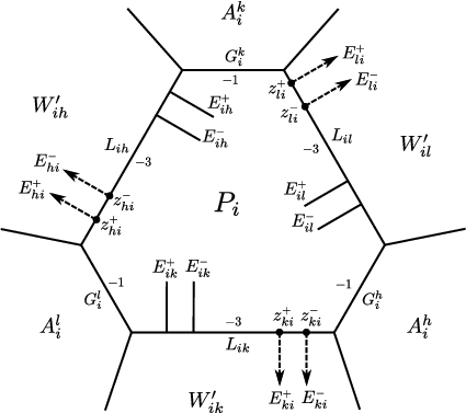
The central fibre of the intermediate family $\pi:{X}\to\Delta$ is pictured in Figure 1 (p. 1; we provide a cylindrical projection of a real picture of $X_{0}$ , the dual graph of which is topologically an $\mathbf{S}^{2}$ sphere), and the flops are described in Figure 2 (p. 2). The reason why we need to make the degree 6 base change is, intuitively, the following: a degree $3$ base change is needed to understand the contribution to the limit Severi variety of curves passing through a vertex (i.e. a triple point) of the tetrahedron, while an additional degree $2$ base change enables one to understand the contributions due to the edges (i.e. the double lines) of the tetrahedron.

Steps (I) and (II)

The singularities of the initial total space $S$ consist of four ordinary double points on each edge of $S_{0}$ . We consider (cf. Example 2.1) the small resolution $\tilde{S}\to S$ obtained by arranging for every edge the four $(-1)$ –curves two by two on the two adjacent faces. We call $\tilde{f}:\tilde{S}\to\Delta$ the new family.

Let $p_{1},\ldots,p_{4}$ be the triple points of $\tilde{S}_{0}$ . For each $i\in\{1,\ldots,4\}$ , we let $P_{i}$ be the irreducible component of $\tilde{S}_{0}$ which is opposite to the vertex $p_{i}$ : it is a plane blown-up at six points. For distinct $i,j\in\{1,\ldots,4\}$ , we let $E^{\scriptscriptstyle+}_{ij}$ and $E^{\scriptscriptstyle-}_{ij}$ be the two $(-1)$ -curves contained in $P_{i}$ and meeting $P_{j}$ . We call $z^{\scriptscriptstyle+}_{ij}$ and $z^{\scriptscriptstyle-}_{ij}$ the two points cut out on $P_{i}$ by $E^{\scriptscriptstyle+}_{ji}$ and $E^{\scriptscriptstyle-}_{ji}$ respectively.

Let now $\bar{f}:\bar{S}\to\Delta$ be the family obtained from $\tilde{f}:\tilde{S}\to\Delta$ by the base change $t\in\Delta\mapsto t^{6}\in\Delta$ . The central fibre $\bar{S}_{0}$ is isomorphic to $\tilde{S}_{0}$ , so we will keep the above notation for it.

Step (III)

As a first step in the desingularization of $\bar{S}$ , we perform the following sequence of operations for all $i\in\{1,\ldots,4\}$ . The total space $\bar{S}$ around $p_{i}$ is locally analytically isomorphic to the hypersurface of $\mathbf{C}^{4}$ defined by the equation $xyz=t^{6}$ at the origin. We blow-up $\bar{S}$ at $p_{i}$ . The blown–up total space locally sits in $\bf C^{4}\times\mathbf{P}^{3}$ . Let $(\xi:\eta:\zeta:\vartheta)$ be the homogeneous coordinates in $\bf P^{3}$ . Then the new total space is locally defined in $\bf C^{4}\times\mathbf{P}^{3}$ by the equations

\xi^{4}\eta\zeta=\vartheta^{6}x^{3},\quad\xi\eta^{4}\zeta=\vartheta^{6}y^{3},\quad\xi\eta\zeta^{4}=\vartheta^{6}z^{3},\quad\text{and}\quad\xi\eta\zeta=\vartheta^{3}t^{3}.

(4.1)

The equation of the exceptional divisor (in the exceptional $\bf P^{3}$ of the blow–up of $\bf C^{4}$ ) is $\xi\eta\zeta=0$ , hence this is the union of three planes meeting transversely at a point $p^{\prime}_{i}$ in $\bf P^{3}$ . For $i,j$ distinct in $\{1,\ldots,4\}$ , we call $A_{j}^{i}$ the exceptional planes meeting the proper transform of $P_{j}$ (which, according to our conventions, we still denote by $P_{j}$ , see §1).

The equation of the new family around the point $p^{\prime}_{i}$ given by $\bigcap_{j\neq i}A_{j}^{i}$ is $\xi\eta\zeta=t^{3}$ (which sits in the affine chart $\vartheta=1$ ). Next we blow-up the points $p^{\prime}_{i}$ , for $i\in\{1,\ldots,4\}$ . The new exceptional divisor $T^{i}$ at each point $p^{\prime}_{i}$ is isomorphic to the cubic surface with equation $\xi\eta\zeta=t^{3}$ in the $\mathbf{P}^{3}$ with coordinates $(\xi:\eta:\zeta:t)$ . Note that $T^{i}$ has three $A_{2}$ –double points, at the vertices of the triangle $t=0,\,\,\xi\eta\zeta=0$ .

Next we have to get rid of the singularities of the total space along the double curves of the central fibre. First we take care of the curves $C_{hk}:=P_{h}\cap P_{k}$ , for $h,k$ distinct in $\{1,\ldots,4\}$ . The model we constructed so far is defined along such a curve by an equation of the type $\xi\eta=\vartheta^{6}z^{3}$ , (as it follows, e.g., from the third equation in (4.1) by setting $\zeta=1$ ). The curve $C_{hk}$ is defined by $\xi=\eta=\vartheta=0$ . If $i\in\{1,\ldots,4\}-\{h,k\}$ , the intersection point $p_{hki}:=C_{hk}\cap A_{h}^{i}\cap A_{k}^{i}$ is cut out on $C_{hk}$ by the hyperplane with equation $z=0$ . Away from the $p_{hki}$ ’s, with $i\in\{1,\ldots,4\}-\{h,k\}$ , the points of $C_{hk}$ are double points of type $A_{5}$ for the total space. We blow–up along this curve: this introduces new homogeneous coordinates $(\xi_{1}:\eta_{1}:\vartheta_{1})$ , with new equations for the blow–up

\xi_{1}^{5}\eta_{1}=\vartheta_{1}^{6}\xi^{4}z^{3},\quad\xi_{1}\eta_{1}^{5}=\vartheta_{1}^{6}\eta^{4}z^{3},\quad\text{and}\quad\xi_{1}\eta_{1}=\vartheta_{1}^{2}\vartheta^{4}z^{3}.

The exceptional divisor is defined by $\xi_{1}\eta_{1}=0$ , and is the transverse union of two ruled surfaces: we call $W_{hk}^{\prime}$ the one that meets $P_{h}$ , and $W_{kh}^{\prime}$ the other. The affine chart we are interested in is $\vartheta_{1}=1$ , where the equation is $\xi_{1}\eta_{1}=\vartheta^{4}z^{3}$ . We then blow–up along the curve $\xi_{1}=\eta_{1}=\vartheta=0$ , which gives in a similar way the new equation $\xi_{2}\eta_{2}=\vartheta^{2}z^{3}$ with the new coordinates $(\xi_{2}:\eta_{2}:\vartheta_{2})$ . The exceptional divisor consists of two ruled surfaces, and we call $W_{hk}^{\prime\prime}$ (resp. $W_{kh}^{\prime\prime}$ ) the one that meets $W_{hk}^{\prime}$ (resp. $W_{kh}^{\prime}$ ). Finally, by blowing-up along the curve $\xi_{2}=\eta_{2}=\vartheta=0$ , we obtain a new equation $\xi_{3}\eta_{3}=\vartheta_{3}^{2}z^{3}$ , with new coordinates $(\xi_{3}:\eta_{3}:\vartheta_{3})$ . The exceptional divisor is a ruled surface, with two $A_{2}$ –double points at its intersection points with the curves $C^{i}_{hk}:=A_{h}^{i}\cap A_{k}^{i}$ , with $i\in\{1,\ldots,4\}-\{h,k\}$ . We call it either $W_{hk}$ or $W_{kh}$ , with no ambiguity.

The final step of our desingularization process consists in blowing–up along the twelve curves $C^{i}_{hk}$ , with pairwise distinct $h,k,i\in\{1,\ldots,4\}$ . The total space is given along each of these curves by an equation of the type $\xi\eta=\vartheta^{3}t^{3}$ in the variables $(\xi,\eta,\theta,t)$ , obtained from the last equation in (4.1) by setting $\zeta=1$ . The curve $C^{i}_{hk}$ is defined by the local equations $\xi=\eta=t=0$ , which shows that they consist of $A_{2}$ –double points for the total space. They also contain an $A_{2}$ –double point of $W_{hk}$ and $T^{i}$ respectively. A computation similar to the above shows that the blow–up along these curves resolves all singularities in a single move. The exceptional divisor over $C^{i}_{hk}$ is the union of two transverse ruled surfaces: we call $V_{hk}^{i}$ the one that meets $A_{h}^{i}$ , and $V_{kh}^{i}$ the other.

At this point, we have a semistable family $\pi:X\to\Delta$ , whose central fibre is depicted in Figure 1: for each double curve we indicate its self–intersections in the two components of the central fibre it belongs to. This is obtained by applying the Triple Point Formula (see Lemma 2.2).

Refer to caption — Figure 1: Planisphere of the model $X_{0}$ of the degeneration into four planes

Step (IV)

For our purposes, we need to further blow-up the total space along the twelve curves $\Gamma^{i}_{hk}:=V_{hk}^{i}\cap V_{kh}^{i}$ . This has the drawback of introducing components with multiplicity two in the central fibre, namely the corresponding exceptional divisors. To circumvent this, we will flop these curves as follows.

Let $\hat{\pi}:\hat{X}\to\Delta$ be the family obtained by blowing-up $X$ along the $\Gamma^{i}_{hk}$ ’s. We call $W_{hk}^{i}$ (or, unambiguously, $W_{kh}^{i}$ ) the corresponding exceptional divisors: they appear with multiplicity two in the central fibre $\hat{X}_{0}$ . By applying the Triple Point Formula as in Remark 2.3, one checks that the surfaces $W_{kh}^{i}$ are all isomorphic to $\mathbf{P}^{1}\times\mathbf{P}^{1}$ . Moreover, it is possible to contract $W_{hk}^{i}$ in the direction of the ruling cut out by $V_{hk}^{i}$ and $V_{kh}^{i}$ , as indicated on Figure 2. We call $\hat{X}\to\bar{X}$ the contraction of the twelve divisors $W_{hk}^{i}$ in this way, and $\varpi:\bar{X}\to\Delta$ the corresponding semistable family of surfaces.

Even though $\bar{X}\dashrightarrow X$ is only a birational map, we have a birational morphism $\bar{X}\to\bar{S}$ over $\Delta$ .

Identification of the components of the central fibre

Summarizing, the irreducible components of the central fibre $\bar{X}_{0}$ are the following:

(i) The 4 surfaces $P_{i}$ , with $1\leqslant i\leqslant 4$ .

Each $P_{i}$ is a plane blown–up at 6+3 points, and $H$ (i.e. the pull-back of a general line in the plane, recall our conventions in §1) is the restriction class of $\mathcal{O}_{\bar{X}}(1)$ on $P_{i}$ . For $j,k\in\{1,\ldots,4\}-\{i\}$ , we set

L_{ij}:=P_{i}\cap W_{ij}^{\prime}\quad{\rm and}\quad G^{k}_{i}:=P_{i}\cap A_{i}^{k},

as indicated in Figure 4. In addition to the three $(-1)$ –curves $G_{i}^{k}$ , we have on $P_{i}$ the six exceptional curves $E^{\scriptscriptstyle+}_{ij},E^{\scriptscriptstyle-}_{ij}$ , for all $j\in\{1,\ldots,4\}-\{i\}$ , with $E^{\scriptscriptstyle+}_{ij},E^{\scriptscriptstyle-}_{ij}$ intersecting $L_{ij}$ at one point. Moreover, for $j\in\{1,\ldots,4\}-\{i\}$ , we have on $L_{ij}$ the two points $z^{\scriptscriptstyle\pm}_{ji}$ defined as the strict transform of the intersection $E^{\scriptscriptstyle\pm}_{ji}\cap L_{ij}$ in $\tilde{S}$ . We will denote by $Z_{i}$ the $0$ –dimensional scheme of length 6 given by $\sum_{j\neq i}(z^{\scriptscriptstyle+}_{ji}+z^{\scriptscriptstyle-}_{ji})$ . We let $\mathcal{I}_{Z_{i}}\subset\mathcal{O}_{P_{i}}$ be its defining sheaf of ideals.

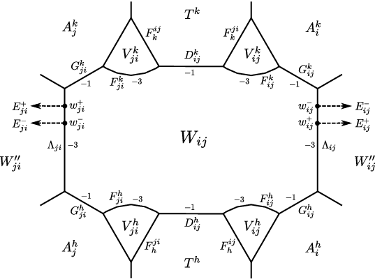
(ii) The 24 surfaces $W^{\prime}_{ij},W^{\prime\prime}_{ij}$ , with $i,j\in\{1,\ldots,4\}$ distinct.

Each of them is isomorphic to ${\bf F}_{1}$ . We denote by $|F|$ the ruling. Note that the divisor class $F$ corresponds to the restriction of $\mathcal{O}_{\bar{X}}(1)$ .

(iii) The 6 surfaces $W_{ij}$ , with $i,j\in\{1,\ldots,4\}$ distinct.

For each $k\in\{1,\ldots,4\}-\{i,j\}$ , we set

\Lambda_{ij}:=W_{ij}^{\prime\prime}\cap{W_{ij}},\quad G_{ij}^{k}:=W_{ij}\cap A_{i}^{k},\quad F_{ij}^{k}=W_{ij}\cap V_{ij}^{k},\quad D_{ij}^{k}=W_{ij}\cap T^{k},

and define similarly $\Lambda_{ji}$ , $G_{ji}^{k}$ , $F_{ji}^{k}$ ( $D_{ij}^{k}$ may be called $D_{ji}^{k}$ without ambiguity). This is indicated in Figure 4.

A good way of thinking to the surfaces $W_{ij}$ is to consider them as (non–minimal) rational ruled surfaces, for which the two curves $\Lambda_{ji}$ and $\Lambda_{ij}$ are sections which do not meet, and the two rational chains

G_{ji}^{k}+F_{ji}^{k}+2D_{ij}^{k}+F_{ij}^{k}+G_{ij}^{k},\quad k\in\{1,\ldots,4\}-\{i,j\},

are two disjoint reducible fibres of the ruling $|F|$ . One has furthermore $\mathcal{O}_{W_{ij}}(F)=\mathcal{O}_{\bar{X}}(1)\otimes\mathcal{O}_{W_{ij}}$ .

The surface $W_{ij}$ has the length 12 anticanonical cycle

\Lambda_{ji}+G_{ji}^{k}+F_{ji}^{k}+D_{ij}^{k}+F_{ij}^{k}+G_{ij}^{k}+\Lambda_{ij}+G_{ij}^{h}+F_{ij}^{h}+D_{ij}^{h}+F_{ji}^{h}+G_{ji}^{h}

(4.2)

cut out by $\bar{X}_{0}-W_{ij}$ , where we fixed $k$ and $h$ such that $\{i,j,k,h\}=\{1,\ldots,4\}$ . It therefore identifies with a plane blown–up as indicated in Figure 5: consider a general triangle $L_{1},L_{2},L_{3}$ in $\mathbf{P}^{2}$ , with vertices $a_{1},a_{2},a_{3}$ , where $a_{1}$ is opposite to $L_{1}$ , etc.; then blow–up the three vertices $a_{s}$ , and call $E_{s}$ the corresponding exceptional divisors; eventually blow–up the six points $L_{r}\cap E_{s}$ , $r\neq s$ , and call $E_{rs}$ the corresponding exceptional divisors. The obtained surface has the anticanonical cycle

L_{1}+E_{13}+E_{1}+E_{23}+L_{2}+E_{21}+E_{1}+E_{31}+L_{3}+E_{32}+E_{2}+E_{12},

(4.3)

which we identify term-by-term and in this order with the anticanonical cycle (4.2) of $W_{ij}$ .

We let $H$ be, as usual, (the transform of) a general line in the plane

H\sim_{W_{ij}}\;\Lambda_{ji}+\sum\nolimits_{k\not\in\{i,j\}}(2G_{ji}^{k}+F_{ji}^{k}+D_{ji}^{k}).

(4.4)

The ruling $|F|$ is the strict transform of the pencil of lines through the point $a_{1}$ , hence

|F|=\bigl|H-(\Lambda_{ij}+G_{ij}^{k}+G_{ij}^{h})\bigr|,\quad\text{with}\quad\{1,\ldots,4\}=\{i,j,k,h\}.

(4.5)

(iv) The 4 surfaces $T^{k}$ , with $1\leqslant k\leqslant 4$ .

Here we set

\Gamma^{k}_{i}=T^{k}\cap A^{k}_{i},\ \text{for}\ i\in\{1,\ldots,4\}-\{k\},\quad\text{and}\quad F_{k}^{ij}=T^{k}\cap V^{k}_{ij},\ \text{for}\ i,j\in\{1,\ldots,4\}-\{k\}\ {\rm distinct}.

Also recall that $D_{ij}^{k}=T^{k}\cap W_{ij}$ for $i,j\in\{1,\ldots,4\}-\{k\}$ distinct. This is indicated in Figure 6.

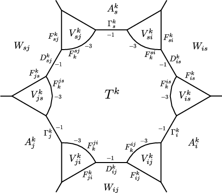
Each $T^{k}$ identifies with a plane blown–up as indicated in Figure 5, as in the case of the $W_{ij}$ ’s: it has the length 12 anticanonical cycle

F_{k}^{js}+D_{sj}^{k}+F_{k}^{sj}+\Gamma_{s}^{k}+F_{k}^{si}+D^{k}_{is}+F_{k}^{is}+\Gamma^{k}_{i}+F_{k}^{ij}+D_{ij}^{k}+F_{k}^{ji}+\Gamma^{k}_{j}

(4.6)

(where we fixed indices $s,i,j$ such that $\{s,i,j,k\}=\{1,\ldots,4\}$ ) cut out by $\bar{X}_{0}-T^{k}$ on $T^{k}$ , which we identify term-by-term and in this order with the anticanonical cycle (4.3). This yields

H\sim_{T^{k}}\;F_{k}^{js}+(2D_{sj}^{k}+F_{k}^{sj}+\Gamma_{s}^{k})+(2\Gamma_{j}^{k}+F_{k}^{ji}+D_{ij}^{k}).

(4.7)

We have on $T^{k}$ the proper transform of a pencil of (bitangent) conics that meet the curves $\Gamma_{s}^{k}$ and $D_{ij}^{k}$ in one point respectively, and do not meet any other curve in the anticanonical cycle (4.6): we call this pencil $|\Phi^{k}_{s}|$ , and we have

\bigl|\Phi^{k}_{s}\bigr|=\bigl|2H-(F_{k}^{sj}+D_{sj}^{k}+2\Gamma_{s}^{k})-(F_{k}^{ji}+\Gamma_{j}^{k}+2D_{ij}^{k})\bigr|.

The restriction of $\mathcal{O}_{\bar{X}}(1)$ on $T^{k}$ is trivial.

(v) The 12 surfaces $A^{k}_{i}$ , with $i,k\in\{1,\ldots,4\}$ distinct.

Each of them identifies with a blown–up plane as indicated in Figure 7. It is equipped with the ruling $|H-\Gamma_{i}^{k}|$ , the members of which meet the curves $G_{i}^{k}$ and $\Gamma_{i}^{k}$ at one point respectively, and do not meet any other curve in the length 8 anticanonical cycle cut out by $\bar{X}_{0}-A_{i}^{k}$ on $A_{i}^{k}$ . The restriction of $\mathcal{O}_{\bar{X}}(1)$ on $A_{i}^{k}$ is trivial.

(vi) The 24 surfaces $V^{k}_{ij}$ with $i,j,k\in\{1,\ldots 4\}$ distinct.

These are all copies of $\mathbf{P}^{2}$ , on which the restriction of $\mathcal{O}_{\bar{X}}(1)$ is trivial.

The limit linear system, I: construction

According with the general principles stated in §2.2, we shall now describe the limit linear system of $|\mathcal{O}_{\bar{X}_{t}}(1)|$ as $t\in\Delta^{*}$ tends to $0$ . This will suffice for the proof, presented in §4.7, that $\varpi:\bar{X}\to\Delta$ is a $\delta$ –good model for $1\leqslant\delta\leqslant 3$ .

We start with ${\mathfrak{P}}:=\mathbf{P}(\varpi_{*}(\mathcal{O}_{\bar{X}}(1)))$ , which is a $\mathbf{P}^{3}$ –bundle over $\Delta$ , whose fibre at $t\in\Delta$ is $|\mathcal{O}_{\bar{X}_{t}}(1)|$ . We set $\mathcal{L}=\mathcal{O}_{\bar{X}}(1)$ , and $|\mathcal{O}_{\bar{X}_{t}}(1)|=|\mathcal{L}_{t}|$ ; note that $|\mathcal{L}_{0}|\cong|\mathcal{O}_{S_{0}}(1)|$ . We will often use the same notation to denote a divisor (or a divisor class) on the central fibre and its restriction to a component of the central fibre, if this does not cause any confusion.

We will proceed as follows:

(I) we first blow–up

\mathfrak{P}

at the points

\pi_{i}

corresponding to the irreducible components

P_{i}

S_{0}

, for

i\in\{1,\ldots,4\}

(the new central fibre then consists of

|\mathcal{O}_{S_{0}}(1)|\cong\bf P^{3}

blown–up at four independent points, plus the four exceptional

\mathbf{P}^{3}

’s);
(II) next, we blow–up the total space along the proper transforms

\ell_{ij}

of the six lines of

|\mathcal{O}_{S_{0}}(1)|

joining two distinct points

\pi_{i},\pi_{j}

, with

i,j\in\{1,\ldots,4\}

, corresponding to pencils of planes with base locus an edge of

S_{0}

(the new central fibre is the proper transform of the previous one, plus the six exceptional

\mathbf{P}\bigl(\mathcal{O}_{\mathbf{P}^{1}}\oplus\mathcal{O}_{\mathbf{P}^{1}}(1)^{\oplus 2}\bigr)

’s);
(III) finally, we further blow–up along the proper transforms of the planes

\Pi_{k}

corresponding to the webs of planes passing through the vertices

p_{k}

S_{0}

, for

k\in\{1,\ldots,4\}

(this adds four more exceptional divisors to the central fibre, for a total of fifteen irreducible components).

In other words, we successively blow–up $\mathfrak{P}$ along all the cells of the tetrahedron dual to $S_{0}$ in $\mathfrak{P}_{0}$ , by increasing order of dimension.

Each of these blow–ups will be interpreted in terms of suitable twisted linear systems as indicated in Remark 2.5. It will then become apparent that every point in the central fibre of the obtained birational modification of $\mathfrak{P}$ corresponds to a curve in $\bar{X}_{0}$ (see §4.7), and hence that this modification is indeed the limit linear system $\mathfrak{L}$ .

Step (I)

In $\mathrm{H}^{0}(\bar{X}_{0},\mathcal{O}_{\bar{X}_{0}}(1))$ there is for each $i\in\{1,\ldots,4\}$ the 1–dimensional subspace of sections vanishing on $P_{i}$ , which corresponds to the sections of $\mathrm{H}^{0}(S_{0},\mathcal{O}_{S_{0}}(1))$ vanishing on the plane $P_{i}$ . As indicated in Remark 2.5, in order to construct the limit linear system, we have to blow up the corresponding points $\pi_{i}\in|\mathcal{L}_{0}|$ . Let ${\mathfrak{P}}^{\prime}\to{\mathfrak{P}}$ be this blow–up, and call $\tilde{\mathfrak{L}}_{i}$ , $1\leqslant i\leqslant 4$ , the exceptional divisors. Each $\tilde{\mathfrak{L}}_{i}$ is a $\mathbf{P}^{3}$ , and can be interpreted as the trace of the linear system $\bigl|\mathcal{L}_{0}(-P_{i})\bigr|$ on $X_{0}$ (see Lemma 2.7 and Example 2.8). However, any section of $\mathrm{H}^{0}(\bar{X}_{0},\mathcal{L}_{0}(-P_{i}))$ still vanishes on components of $\bar{X}_{0}$ different from $P_{i}$ . By subtracting all of them with the appropriate multiplicities (this computation is tedious but not difficult and can be left to the reader), one sees that $\tilde{\mathfrak{L}}_{i}$ can be identified as the linear system $\mathfrak{L}_{i}:=\bigl|\mathcal{L}_{0}(-M_{i})\bigr|$ , where

M_{i}:=6P_{i}+\sum_{j\neq i}(5W_{ij}^{\prime}+4W_{ij}^{\prime\prime}+3W_{ij}+2W_{ji}^{\prime\prime}+W_{ji}^{\prime})+\\ +\sum_{k\neq i}\Biggl(2T^{k}+4A_{i}^{k}+\sum_{j\not\in\{i,k\}}\left(3V_{ij}^{k}+2V_{ji}^{k}+A_{j}^{k}\right)+\sum_{\{j<\bar{\jmath}\}\cap\{i,k\}=\emptyset}\left(V_{j\bar{\jmath}}^{k}+V_{\bar{\jmath}j}^{k}\right)\Biggr).

(4.8)

With the notation introduced in §4.2, one has:

Lemma 4.1

The restriction class of $\mathcal{L}_{0}(-M_{i})$ to the irreducible components of $\bar{X}_{0}$ is as follows:

(i) on

P_{i}

, we find

4H-\sum_{j\neq i}(E^{\scriptscriptstyle+}_{ij}+E^{\scriptscriptstyle-}_{ij})

;
(ii) on

P_{j}

j\neq i

, we find

E^{\scriptscriptstyle+}_{ji}+E^{\scriptscriptstyle-}_{ji}

;
(iii) for each

j\neq i

, we find

2F

on each of the surfaces

W_{ij}^{\prime}

W_{ij}^{\prime\prime}

W_{ij}

W_{ji}^{\prime\prime}

W_{ji}^{\prime}

.
(iv) on the remaining components the restriction is trivial.

Proof.

This is a tedious but standard computation. As a typical sample we prove (iii), and leave the remaining cases to the reader. Set $\{h,k\}=\{1,\ldots,4\}-\{i,j\}$ . Then, recalling (4.4) and (4.5), we see that the restriction of $\mathcal{L}_{0}(-M_{i})$ to $W_{ij}$ is the line bundle determined by the divisor class

F+\Bigl(W_{ji}^{\prime\prime}-W_{ij}^{\prime\prime}+\sum_{k\not\in\{i,j\}}\bigl(2A_{j}^{k}+V_{ji}^{k}+T^{k}-A_{i}^{k}\bigr)\Bigr)\biggr|_{W_{ij}}\\ \begin{aligned} &\sim F+\Lambda_{ji}-\Lambda_{ij}+(2G_{ji}^{k}+F_{ji}^{k}+D_{ij}^{k}-G_{ij}^{k})+(2G_{ji}^{h}+F_{ji}^{h}+D_{ij}^{h}-G_{ij}^{h})\\ &=F+\bigl(\Lambda_{ji}+(2G_{ji}^{k}+F_{ji}^{k}+D_{ij}^{k})+(2G_{ji}^{h}+F_{ji}^{h}+D_{ij}^{h})\bigr)-(\Lambda_{ij}+G_{ij}^{k}+G_{ij}^{h})=2F.\\ \end{aligned}

∎

From this, we deduce that $\mathfrak{L}_{i}$ identifies with its restriction to $P_{i}$ :

Proposition 4.2

There is a natural isomorphism

\mathfrak{L}_{i}\cong\Bigl|\mathcal{O}_{P_{i}}\Bigl(4H-\sum\nolimits_{j\neq i}(E^{\scriptscriptstyle+}_{ij}+E^{\scriptscriptstyle-}_{ij})\Bigr)\otimes{\cal I}_{Z_{i}}\Bigr|.

(4.9)

Proof.

For each $j\neq i$ , the restriction of $\mathfrak{L}_{i}$ to $P_{j}$ has $E^{\scriptscriptstyle+}_{ji}+E^{\scriptscriptstyle-}_{ji}$ as its only member. This implies that its restriction to $W_{ji}^{\prime}$ has only one member as well, which is the sum of the two curves in $|F|$ intersecting $E^{\scriptscriptstyle+}_{ji}$ and $E^{\scriptscriptstyle-}_{ji}$ respectively. On $W_{ji}^{\prime\prime}$ , we then only have the sum of the two curves in $|F|$ intersecting the two curves on $W_{ji}^{\prime}$ respectively, and so on on $W_{ij}$ , $W_{ij}^{\prime\prime}$ , and $W_{ij}^{\prime}$ . Now the two curves on $W_{ij}^{\prime}$ impose the two base points $z^{\scriptscriptstyle+}_{ji}$ and $z^{\scriptscriptstyle-}_{ji}$ to the restriction of $\mathfrak{L}_{i}$ to $P_{i}$ . The right hand side in (4.9) being $3$ –dimensional, this ends the proof with (i) of Lemma 4.1. ∎

Step (II)

Next, we consider the blow–up ${\mathfrak{P}}^{\prime\prime}\to{\mathfrak{P}}^{\prime}$ along the proper transforms $\ell_{ij}$ of the six lines of $|\mathcal{L}_{0}|$ joining two distinct points $\pi_{i},\pi_{j}$ , with $i,j\in\{1,\ldots,4\}$ , corresponding to the pencils of planes in $|\mathcal{O}_{S_{0}}(1)|$ respectively containing the lines $P_{i}\cap P_{j}$ . The exceptional divisors are isomorphic to $\mathbf{P}(\mathcal{O}_{\mathbf{P}^{1}}\oplus\mathcal{O}_{\mathbf{P}^{1}}(1)^{\oplus 2})$ ; we call them $\tilde{\mathfrak{L}}_{ij}$ , $1\leqslant i<j\leqslant 4$ . Arguing as in Step (I) and leaving the details to the reader, we see that $\tilde{\mathfrak{L}}_{ij}$ is in a natural way a birational modification (see §4.5 below) of the complete linear system $\mathfrak{L}_{ij}:=\left|\mathcal{L}_{0}(-M_{ij})\right|$ , where

M_{ij}:=3W_{ij}+(2W_{ji}^{\prime\prime}+W_{ji}^{\prime})+(2W_{ij}^{\prime\prime}+W_{ij}^{\prime})+\\ +\sum_{k\not\in\{i,j\}}\Biggl(2T^{k}+\sum_{s\neq k}A_{s}^{k}+2\left(V_{ji}^{k}+V_{ij}^{k}\right)+\sum_{\begin{subarray}{c}s\in\{i,j\}\\ r\not\in\{i,j,k\}\end{subarray}}\left(V_{sr}^{k}+V_{rs}^{k}\right)\Biggr).

(4.10)

We will denote by $k<h$ the two indices in $\{1,\ldots,4\}-\{i,j\}$ , and go on using the notations introduced in §4.2.

Lemma 4.3

The restriction class of $\mathcal{L}_{0}(-M_{ij})$ to the irreducible components of $\bar{X}_{0}$ is as follows:

(i) on

P_{k}

(resp.

P_{h}

) we find

H-G_{k}^{h}

(resp.

H-G_{h}^{k}

);
(ii) on each of the surfaces

W^{\prime}_{kh}

W^{\prime\prime}_{kh}

W_{kh}

W^{\prime\prime}_{hk}

, and

W^{\prime}_{hk}

, we find

F

;
(iii) on

A_{h}^{k}

(resp.

A_{k}^{h}

) we find

H-\Gamma_{h}^{k}

(resp.

H-\Gamma_{k}^{h}

);
(iv) on

T^{k}

(resp.

T^{h}

), we find

\Phi^{k}_{h}

(resp.

\Phi^{h}_{k}

);
(v) on

P_{i}

(resp.

P_{j}

), we find

E^{\scriptscriptstyle+}_{ij}+E^{\scriptscriptstyle-}_{ij}

(resp.

E^{\scriptscriptstyle+}_{ji}+E^{\scriptscriptstyle-}_{ji}

);
(vi) on

W_{ij}^{\prime},W_{ij}^{\prime\prime},W_{ji}^{\prime\prime},W_{ji}^{\prime}

, we find

2F

;
(vii) on

W_{ij}

, with

H

as in (4.4), we find

4H-2\left(\Lambda_{ij}+G_{ij}^{k}+G_{ij}^{h}\right)-\left(F_{ji}^{k}+G_{ji}^{k}+D_{ij}^{k}\right)-\left(F_{ji}^{h}+G_{ji}^{h}+D_{ij}^{h}\right)-D_{ij}^{k}-D_{ij}^{h};

(viii) on the remaining components the restriction is trivial.

Proof.

As for Lemma 4.1, this is a tedious but not difficult computation. Again we make a sample verification, proving (vii) above. The restriction class is

F+\Bigl(W_{ji}^{\prime\prime}+\sum_{l=k,h}\left(2A_{j}^{l}+V_{ji}^{l}+T^{l}+V_{ij}^{l}+2A_{i}^{l}\right)+W_{ij}^{\prime\prime}|_{W_{ij}}\Bigr)\biggr|_{W_{ij}}\\ \begin{aligned} &\sim F+\Lambda_{ji}+\sum_{l=k,h}\left(2G_{ji}^{l}+F_{ji}^{l}+D_{ij}^{l}+F_{ij}^{l}+2G_{ij}^{l}\right)+\Lambda_{ij}\\ \end{aligned}

which, by taking into account the identification of Figure 5, i.e. with (4.4) and (4.5), is easily seen to be equivalent to the required class. ∎

Let $w^{\scriptscriptstyle\pm}_{ij}\in W_{ij}$ be the two points cut out on $W_{ij}$ by the two connected chains of curves in $|F|_{W_{ij}^{\prime}}\times|F|_{W_{ij}^{\prime\prime}}$ meeting $E^{\scriptscriptstyle\pm}_{ij}$ respectively. We let $w^{\scriptscriptstyle\pm}_{ji}\in W_{ij}$ be the two points defined in a similar fashion by starting with $E^{\scriptscriptstyle\pm}_{ji}$ . Define the $0$ -cycle $Z_{ij}=w^{\scriptscriptstyle+}_{ij}+w^{\scriptscriptstyle-}_{ij}+w^{\scriptscriptstyle+}_{ji}+w^{\scriptscriptstyle-}_{ji}$ on $W_{ij}$ , and let $\mathcal{I}_{Z_{ij}}\subset\mathcal{O}_{W_{ij}}$ be its defining sheaf of ideals.

Proposition 4.4

There is a natural isomorphism between $\mathfrak{L}_{ij}$ and its restriction to $W_{ij}$ , which is the $3$ –dimensional linear system

\Bigl|\mathcal{O}_{W_{ij}}\Bigl(4H-2\left(\Lambda_{ij}+G_{ij}^{k}+G_{ij}^{h}\right)-\left(F_{ji}^{k}+G_{ji}^{k}+D_{ij}^{k}\right)-\left(F_{ji}^{h}+G_{ji}^{h}+D_{ij}^{h}\right)-D_{ij}^{k}-D_{ij}^{h}\Bigr)\otimes\mathcal{I}_{Z_{ij}}\Bigr|,

(4.11)

where we set $\{1,\ldots,4\}=\{i,j,h,k\}$ , and $H$ as in (4.4).

Proof.

Consider a triangle $L_{1},L_{2},L_{3}$ in $\mathbf{P}^{2}$ , with vertices $a_{1},a_{2},a_{3}$ , where $a_{1}$ is opposite to $L_{1}$ , etc. Consider the linear system $\mathcal{W}$ of quartics with a double point at $a_{1}$ , two simple base points infinitely near to $a_{1}$ not on $L_{2}$ and $L_{3}$ , two base points at $a_{2}$ and $a_{3}$ with two infinitely near base points along $L_{3}$ and $L_{2}$ respectively, two more base points along $L_{1}$ . There is a birational transformation of $W_{ij}$ to the plane (see Figure 5) mapping (4.11) to a linear system of type $\mathcal{W}$ . One sees that two independent conditions are needed to impose to the curves of $\mathcal{W}$ to contain the three lines $L_{1},L_{2},L_{3}$ and the residual system consists of the pencil of lines through $a_{1}$ . This proves the dimensionality assertion (see §4.5 below for a more detailed discussion).

Consider then the restriction of $\mathfrak{L}_{ij}$ to the chain of surfaces

P_{j}+W_{ji}^{\prime}+W_{ji}^{\prime\prime}+W_{ij}+W_{ij}^{\prime\prime}+W_{ij}^{\prime}+P_{i}.

By taking into account (v), (vi), and (vii), of Lemma 4.3, we see that each divisor $C$ of this system determines, and is determined, by its restriction $C^{\prime}$ on $W_{ij}$ , since $C$ consists of $C^{\prime}$ plus four rational tails matching it.

The remaining components of $\bar{X}_{0}$ on which $\mathfrak{L}_{ij}$ is non–trivial, all sit in the chain

T^{k}+A^{k}_{h}+P_{h}+W_{lk}^{\prime}+W_{lk}^{\prime\prime}+W_{hk}+W_{kh}^{\prime\prime}+W_{kh}^{\prime}+P_{k}+A^{h}_{k}+T^{h}.

(4.12)

The restrictions of $\mathfrak{L}_{ij}$ to each irreducible component of this chain is a base point free pencil of rational curves, hence $\mathfrak{L}_{ij}$ restricts on (4.12) to the $1$ –dimensional system of connected chains of rational curves in these pencils: we call it $\mathfrak{N}^{kh}$ . Given a curve in $\mathfrak{L}_{ij}$ , it cuts $T^{k}$ and $T^{h}$ in one point each, and there is a unique chain of rational curves in $\mathfrak{N}^{kh}$ matching these two points. ∎

Step (III)

Finally, we consider the blow-up ${\mathfrak{P}}^{\prime\prime\prime}\to{\mathfrak{P}}^{\prime\prime}$ along the proper transforms of the three planes that are strict transforms of the webs of planes in $|\mathcal{O}_{S_{0}}(1)|$ containing a vertex $p_{k}$ , with $1\leqslant k\leqslant 4$ . For each $k$ , the exceptional divisor $\tilde{\mathfrak{L}}^{k}$ is a birational modification (see §4.6 below) of the complete linear system $\mathfrak{L}^{k}:=\bigl|\mathcal{L}_{0}(-M^{k})\bigr|$ , where

M^{k}:=2T^{k}+\sum_{s\neq k}A_{s}^{k}+\sum_{\{s<r\}\not\ni k}\left(V_{sr}^{k}+V_{rs}^{k}\right).

Lemma 4.5

The restriction class of $\mathcal{L}_{0}(-M^{k})$ to the irreducible components of $\bar{X}_{0}$ is as follows:

(i) on

P_{i}

i\neq k

, we find

H-G^{k}_{i}

;
(ii) on

A^{k}_{i}

i\neq k

, we find

H-\Gamma_{i}^{k}

;
(iii) on

P_{k}

, as well as on the chains

W_{ik}^{\prime}+W_{ik}^{\prime\prime}+W_{ik}+W_{ki}^{\prime\prime}+W_{ki}^{\prime}

i\neq k

, we find the restriction class of

\mathcal{L}_{0}

;
(iv) on

T^{k}

, we find

3H-(F_{k}^{sj}+D^{k}_{sj}+2\Gamma_{s}^{k})-(F_{k}^{ji}+D_{ij}^{k}+2\Gamma_{j}^{k})-(F_{k}^{is}+D_{is}^{k}+2\Gamma_{i}^{k}),

with

\{s,i,j,k\}=\{1,\ldots,4\}

, and

H

as in (4.7);
(v) on the remaining components it is trivial.

Proof.

We limit ourselves to a brief outline of how things work for $T^{k}$ . The restriction class is

\Bigl(\sum_{r\neq k}A_{r}^{k}+\sum_{\{r<r^{\prime}\}\not\ni k}\left(V_{rr^{\prime}}^{k}+2W_{rr^{\prime}}+V_{r^{\prime}r}^{k}\right)\Bigr)\biggr|_{T^{k}}

which is seen to be equal to the required class with the identification of Figures 5 and 6, i.e. with $H$ as in (4.7). ∎

Proposition 4.6

There is a natural isomorphism between $\mathfrak{L}^{k}$ and its restriction to $T^{k}$ , which is the $3$ –dimensional linear system

\bigl|3H-(F_{k}^{sj}+D^{k}_{sj}+2\Gamma_{s}^{k})-(F_{k}^{ji}+D_{ij}^{k}+2\Gamma_{j}^{k})-(F_{k}^{is}+D_{is}^{k}+2\Gamma_{i}^{k})\bigr|,

where we set $\{s,i,j,k\}=\{1,\ldots,4\}$ , and $H$ as in (4.7).

Proof.

This is similar (in fact, easier) to the proof of Proposition 4.4, so we will be sketchy here. The dimensionality assertion will be discussed in §4.6 below.

For each $i\neq k$ , the restriction of $\mathfrak{L}^{k}$ to each irreducible component of the chain

A^{k}_{i}+P_{i}+W_{ik}^{\prime}+W_{ik}^{\prime\prime}+W_{ik}+W_{ki}^{\prime\prime}+W_{ki}^{\prime}

(4.13)

is a base point free pencil of rational curves, and $\mathfrak{L}^{k}$ restricts on (4.13) to the $1$ –dimensional system of connected chains of rational curves in these pencils, that we will call $\mathfrak{N}^{k}_{i}$ .

Now the general member of $\mathfrak{L}^{k}$ consists of a curve in $\mathfrak{L}^{k}\bigr|_{T^{k}}$ , which uniquely determines three chains of rational curves in $\mathfrak{N}^{k}_{i}$ , $i\neq k$ , which in turn determine a unique line in $|\mathcal{O}_{P^{k}}(H)|$ . ∎

The linear systems $\mathfrak{L}_{i}$ .

Let $a,b,c$ be three independent lines in $\mathbf{P}^{2}$ , and consider a $0$ –dimensional scheme $Z$ cut out on $a+b+c$ by a general quartic curve. Consider the linear system $\mathcal{P}$ of plane quartics containing $Z$ . This is a linear system of dimension 3. Indeed containing the union of the three lines $a,b,c$ is one condition for the curves in $\mathcal{P}$ and the residual system is the $2$ –dimensional complete linear system of all lines in the plane.

Proposition 4.2 shows that $\mathfrak{L}_{i}$ can be identified with a system of type $\mathcal{P}$ . We denote by $\sigma_{i}:P_{i}\dasharrow\mathbf{P}^{3}$ (or simply by $\sigma$ ) the rational map determined by $\mathfrak{L}_{i}$ and by $Y$ its image, which is the same as the image of the plane via the rational map determined by the linear system $\mathcal{P}$ .

Proposition 4.7

The map $\sigma:P_{i}\dasharrow Y$ is birational, and $Y$ is a monoid quartic surface, with a triple point $p$ with tangent cone consisting of a triple of independent planes through $p$ , and with no other singularity.

Proof.

The triple point $p\in Y$ is the image of the curve $C=\sum_{i=j}^{3}(2D_{i}^{j}+L_{ij})$ (alternatively, of the sides of the triangle $a,b,c$ ). By subtracting $C$ to $\mathfrak{L}_{i}$ one gets a homaloidal net, mapping to the net of lines in the plane. This proves the assertion. ∎

Remark 4.8

The image of $\bar{X}$ by the complete linear system $|\mathcal{L}(-M_{i})|$ provides a model $f^{\prime}:S^{\prime}\to\Delta$ of the initial family $f:S\to\Delta$ , such that the corresponding flat limit of $S^{\prime}_{t}\cong S_{t^{6}}$ with $t\neq 0$ , is $S^{\prime}_{0}=Y$ the quartic monoid image of the face $P_{i}$ of the tetrahedron via $\sigma$ . The map $\bar{X}_{0}\to S^{\prime}_{0}$ contracts all other irreducible components of $\bar{X}_{0}$ to the triple point of the monoid.

Remark 4.9

Theorem D says that the degree of the dual surface of the monoid $Y$ is 21.

The strict transform of $\tilde{\mathfrak{L}}_{i}$ in $\mathfrak{P}_{0}^{\prime\prime\prime}$ (which we still denote by $\tilde{\mathfrak{L}}_{i}$ , see §1) can be identified as a blow–up of $\mathfrak{L}_{i}\cong\mathcal{P}$ : first blow–up the three points corresponding to the three non–reduced curves $2a+b+c$ , $2b+a+c$ , $2c+a+b$ . Then blow–up the proper transforms of the three pencils of lines with centres at $A,B,C$ plus the fixed part $a+b+c$ . We will interpret this geometrically in §4.7, using Lemma 2.7.

The linear systems $\mathfrak{L}_{ij}$ .

Next, we need to study some of the geometric properties of the linear systems $\mathfrak{L}_{ij}$ as in Proposition 4.4. Consider the rational map $\varphi_{ij}:W_{ij}\dasharrow\mathbf{P}^{3}$ (or simply $\varphi$ ) determined by ${\mathfrak{L}}_{ij}$ . Alternatively, one may consider the rational map, with the same image $W$ (up to projective transformations), determined by the planar linear system $\mathcal{W}$ of quartics considered in the proof of Proposition 4.4.

Proposition 4.10

The map $\varphi$ is birational onto its image, which is a quartic surface $W\subset\mathbf{P}^{3}$ , with a double line $D$ , and two triple points on $D$ .

Proof.

First we get rid of the four base points in $Z_{ij}$ by blowing them up and taking the proper transform $\bar{\mathfrak{L}}_{ij}$ of the system. Let $u:\bar{W}\to W_{ij}$ be this blow–up, and let $I^{\scriptscriptstyle\pm}_{ij}$ (resp. $I^{\scriptscriptstyle\pm}_{ji}$ ) be the two $(-1)$ –curves that meet $\Lambda_{ij}$ (resp. $\Lambda_{ji}$ ).

The strict transform $\bar{\mathfrak{L}}_{ij}:=u^{*}({\mathfrak{L}}_{ij})-\left(I^{\scriptscriptstyle+}_{ij}+I^{\scriptscriptstyle-}_{ij}+I^{\scriptscriptstyle+}_{ji}+I^{\scriptscriptstyle-}_{ij}\right)$ , has self–intersection $4$ . Set, as usual, $\{1,\ldots,4\}=\{i,j,h,k\}$ and consider the curves

C_{ji}:=\Lambda_{ji}+(2G_{ji}^{k}+F_{ji}^{k})+(2G_{ji}^{h}+F_{ji}^{h})\quad\text{and}\quad C_{ij}:=\Lambda_{ij}+(2G_{ij}^{k}+F_{ij}^{k})+(2G_{ij}^{h}+F_{ij}^{h}).

(4.14)

One has

\bar{\mathfrak{L}}_{ij}\cdot C_{\bf s}=0,\quad p_{a}(C_{\bf s})=0,\quad C_{\bf s}^{2}=-3,\quad\text{for}\quad{\bf s}\in\{(ij),(ji)\}.

By mapping $\bar{W}$ to $W_{ij}$ , and this to the plane as in Figure 5 with (4.2) and (4.3) identified, one sees that $C_{ji}$ goes to the line $L_{1}$ and $C_{ij}$ to the union of the two lines $L_{2},L_{3}$ . The considerations in the proof of Proposition 4.4 show that $\bar{\mathfrak{L}}_{ij}$ has no base points on $C_{ji}\cup C_{ij}$ (i.e., $\mathcal{W}$ has only the prescribed base points along the triangle $L_{1}+L_{2}+L_{3}$ ). On the other hand, the same considerations show that the base points of $\bar{\mathfrak{L}}_{ij}$ may only lie on $C_{ji}\cup C_{ij}$ . This shows that $\bar{\mathfrak{L}}_{ij}$ is base points free, and the associated morphism $\bar{\varphi}:\bar{W}\to\mathbf{P}^{3}$ contracts $C_{ji}$ and $C_{ij}$ to points $c_{1}$ and $c_{2}$ respectively.

The points $c_{1}$ and $c_{2}$ are distinct, since subtracting the line $L_{1}$ from the planar linear system $\mathcal{W}$ does not force subtracting the whole triangle $L_{1}+L_{2}+L_{3}$ to the system. By subtracting $C_{ji}$ from $\bar{\mathfrak{L}}_{ij}$ , the residual linear system is a linear system of rational curves with self–intersection 1, mapping $W_{ij}$ birationally to the plane. Indeed, this residual linear system corresponds to the residual linear system of $L_{1}$ with respect to $\mathcal{W}$ , which is the linear system of plane cubics, with a double point at $a_{1}$ , two simple base points infinitely near to $a_{1}$ not on $L_{2}$ and $L_{3}$ , two base points at $a_{2}$ and $a_{3}$ , and this is a homaloidal system. This shows that $c_{1}$ is a triple point of $W$ and that $\bar{\varphi}$ is birational. The same for $c_{2}$ . Finally $\bar{\varphi}$ maps (the proper transforms of) $D_{ij}^{k}$ and $D_{ij}^{h}$ both to the unique line $D$ containing $c_{1}$ and $c_{2}$ . ∎

Remark 4.11

The subpencil of $\mathfrak{L}_{ij}$ corresponding to planes in $\mathbf{P}^{3}$ that contain the line $D$ corresponds to the subpencil of curves in $\mathcal{W}$ with the triangle $L_{1}+L_{2}+L_{3}$ as its fixed part, plus the pencil of lines through $a_{1}$ . In this subpencil we have two special curves, namely $L_{1}+2L_{2}+L_{3}$ and $L_{1}+L_{2}+2L_{3}$ . This shows that the tangent cone to $W$ at the general point of $D$ is fixed, formed by two planes.

Remark 4.12

The image of $\bar{X}$ via the complete linear system $|\mathcal{L}(-M_{ij})|$ provides a model $f^{\prime}:S^{\prime}\to\Delta$ of the initial family $f:S\to\Delta$ , such that the corresponding flat limit of $S^{\prime}_{t}\cong S_{t^{6}}$ with $t\neq 0$ , is $S^{\prime}_{0}=W$ the image of $W_{ij}$ via $\varphi$ . The map $\bar{X}_{0}\to S^{\prime}_{0}$ contracts the chain (4.12) to the double line of $W$ , and the two connected components of $\bar{X}_{0}-W_{ij}$ minus the chain (4.12) (cf. Figure 1) to the two triple points of $W$ respectively.

Corollary 4.13

The exceptional divisor $\tilde{\mathfrak{L}}_{ij}$ of ${\mathfrak{P}}^{\prime\prime}\to{\mathfrak{P}}^{\prime}$ is naturally isomorphic to the blow–up of the complete linear system $\bar{\mathfrak{L}}_{ij}\cong\left|\mathcal{O}_{W}(1)\right|$ along its subpencil corresponding to planes in $\mathbf{P}^{3}$ containing the line $D$ .

Proof.

This is a reformulation of the description of $\mathfrak{P}^{\prime\prime}\to\mathfrak{P}^{\prime}$ (cf. Step (II) in §4.3 above), taking into account Propositions 4.4 and 4.10. ∎

The divisor $\tilde{\mathfrak{L}}_{ij}\subset\mathfrak{P}_{0}^{\prime\prime}$ is a $\mathbf{P}(\mathcal{O}_{\mathbf{P}^{1}}(1)^{\oplus 2}\oplus\mathcal{O}_{\mathbf{P}^{1}})$ , and its structure of $\mathbf{P}^{2}$ –bundle over $\mathbf{P}^{1}$ is the minimal resolution of indeterminacies of the rational map $\mathfrak{L}_{ij}\dasharrow|\mathcal{O}_{D}(1)|$ , which sends a general divisor $C\in\mathfrak{L}_{ij}$ to its intersection point with $D$ . The next Proposition provides an identification of the general fibres of $\tilde{\mathfrak{L}}_{ij}$ over $|\mathcal{O}_{D}(1)|=\mathbf{P}^{1}$ as certain linear systems.

Proposition 4.14

The projection of $W$ from a general point of $D$ is a double cover of the plane, branched over a sextic $B$ which is the union

B=B_{0}+B_{1}+B_{2}

of a quartic $B_{0}$ with a node $p$ , and of its tangent cone $B_{1}+B_{2}$ at $p$ , such that the two branches of $B_{0}$ at $p$ both have a flex there (see Figure 8; the intersection $B_{i}\cap B_{0}$ is concentrated at the double point $p$ , for $1\leqslant i\leqslant 2$ ).

Proof.

Let us consider a double cover of the plane as in the statement. It is singular. Following [8, §4], we may obtain a resolution of singularities as a double cover of a blown–up plane with non–singular branch curve. We will then observe that it identifies with $\bar{W}$ blown–up at two general conjugate points on $D_{ij}^{k}$ and $D_{ij}^{h}$ respectively (here conjugate means that the two points are mapped to the same point $x$ of $D$ by $\bar{\varphi}$ ). We will denote by $\tilde{W}$ the surface $\bar{W}$ blown–up at two such points, and by $I_{x}^{\prime},I_{x}^{\prime\prime}$ the two exceptional divisors.

First note that our double plane is rational, because it has a pencil of rational curves, namely the pull-back of the pencil of lines passing through $p$ (eventually this will correspond to the pencil of conics cut out on $W$ by the planes through $D$ ).

In order to resolve the singularities of the branch curve (see Figure 8), we first blow–up $p$ , pull–back the double cover and normalize it. Since $p$ has multiplicity $4$ , which is even, the exceptional divisor $E$ of the blow–up does not belong to the branch curve of the new double cover, which is the proper transform $B$ (still denoted by $B$ according to our general convention). Next we blow–up the two double points of $B$ which lie on $E$ , and repeat the process. Again, the two exceptional divisors $E_{1},E_{2}$ do not belong to the branch curve. Finally we blow–up the two double points of $B$ (which lie one on $E_{1}$ one on $E_{2}$ , off $E$ ), and repeat the process. Once more, the two exceptional divisors $E^{\prime}_{1},E^{\prime}_{2}$ do not belong to the branch curve which is the union of $B_{0}$ , $B_{1}$ and $B_{2}$ (which denote here the proper transforms of the curves with the same names on the plane). This curve is smooth, so the corresponding double cover is smooth.

The final double cover has the following configuration of negative curves: $B_{1}$ (resp. $B_{2}$ ) is contained in the branch divisor, so over it we find a $(-1)$ -curve; $E_{1}^{\prime}$ (resp. $E_{2}^{\prime}$ ) meets the branch divisor at two points, so its pull-back is a $(-2)$ -curve; $E_{1}$ (resp. $E_{2}$ ) does not meet the branch divisor, so its pull-back is the sum of two disjoint $(-2)$ -curves; similarly, the pull-back of $E$ is the sum of two disjoint $(-3)$ -curves. In addition, there are four lines through $p$ tangent to $B_{0}$ and distinct from $B_{1}$ and $B_{2}$ . After the resolution, they are curves with self-intersection $0$ and meet the branch divisor at exactly one point with multiplicity $2$ . The pull-back of any such a curve is the transverse union of two $(-1)$ -curves, each of which meets transversely one component of the pull-back of $E$ .

This configuration is precisely the one we have on $\tilde{W}$ , after the contraction of the four $(-1)$ -curves $G_{ji}^{k}$ , $G_{ij}^{k}$ , $G_{ji}^{h}$ , and $G_{ij}^{h}$ . Moreover, the pull-back of the line class of $\mathbf{P}^{2}$ is the pull–back to $\tilde{W}$ of $\mathfrak{L}_{ij}(-(I_{x}^{\prime}+I_{x}^{\prime\prime}))$ . ∎

Corollary 4.15

In the general fibre of the generic $\mathbf{P}^{2}$ bundle structure of $\tilde{\mathfrak{L}}_{ij}$ , the Severi variety of $1$ –nodal (resp. $2$ –nodal) irreducible curves is an irreducible curve of degree $10$ (resp. the union of $16$ distinct points).

Proof.

This follows from the fact that the above mentioned Severi varieties are respectively the dual curve $\check{B}_{0}$ of a plane quartic as in Proposition 4.14, and the set of ordinary double points of $\check{B}_{0}$ . One computes the degrees using Plücker formulae. ∎

The linear systems $\mathfrak{L}^{k}$

Here we study some geometric properties of the linear systems $\mathfrak{L}^{k}$ appearing in the third step of §4.3.

Consider a triangle $L_{1},L_{2},L_{3}$ in $\mathbf{P}^{2}$ , with vertices $a_{1},a_{2},a_{3}$ , where $a_{1}$ is opposite to $L_{1}$ , etc. Consider the linear system $\mathcal{T}$ of cubics through $a_{1},a_{2},a_{3}$ and tangent there to $L_{3},L_{1},L_{2}$ respectively. By Proposition 4.6, there is a birational transformation of $T^{k}$ to the plane (see Figure 5) mapping $\mathfrak{L}^{k}$ to $\mathcal{T}$ . We consider the rational map $\phi_{k}:T^{k}\dasharrow\mathbf{P}^{3}$ (or simply $\phi$ ) determined by the linear system ${\mathfrak{L}}^{k}$ , or, alternatively, the rational map, with the same image $T$ (up to projective transformations), determined by the planar linear system $\mathcal{T}$ . The usual notation is $\{1,\ldots,4\}=\{i,j,s,k\}$ .

Proposition 4.16

The map $\phi:T^{k}\to T\subset\mathbf{P}^{3}$ is a birational morphism, and $T$ is a cubic surface with three double points of type $A_{2}$ as its only singularities. The minimal resolution of $T$ is the blow–down of $T^{k}$ contracting the $(-1)$ –curves $D^{k}_{ij},D^{k}_{is},D^{k}_{js}$ . This cubic contains exactly three lines, each of them containing two of the double points.

Proof.

The linear system $\mathcal{T}$ is a system of plane cubics with six simple base points, whose general member is clearly irreducible. This implies that $\phi:T^{k}\to T\subset\mathbf{P}^{3}$ is a birational morphism and $T$ is a cubic surface. The linear system $\mathfrak{L}^{k}$ contracts the three chains of rational curves

C_{1}=F_{k}^{js}+2D^{k}_{sj}+F_{k}^{sj},\quad C_{2}=F_{k}^{si}+2D^{k}_{is}+F_{k}^{is},\quad C_{3}=F_{k}^{ij}+2D^{k}_{ij}+F_{k}^{ji},

which map in the plane to the sides of the triangle $L_{1},L_{2},L_{3}$ . By contracting the $(-1)$ –curves $D^{k}_{ij}$ , $D^{k}_{is}$ , $D^{k}_{js}$ , the three curves $C_{1},C_{2},C_{3}$ are mapped to three $(-2)$ –cycles contracted by $\phi$ to double points of type $A_{2}$ .

The rest follows from the classification of cubic hypersurfaces in $\mathbf{P}^{3}$ (see, e.g., [5]). The three lines on $T$ are the images via $\phi$ of the three exceptional divisors $\Gamma^{k}_{i},\Gamma^{k}_{j},\Gamma^{k}_{s},$ . ∎

Remark 4.17

We now see that the image of $\bar{X}$ by the complete linear system $|\mathcal{L}(-M^{k})|$ provides a model $f^{\prime}:S^{\prime}\to\Delta$ of the initial family $f:S\to\Delta$ , such that the corresponding flat limit of $S^{\prime}_{t}\cong S_{t^{6}}$ with $t\neq 0$ , is $S^{\prime}_{0}=T+P$ , where $T$ is the image of $T^{k}$ via $\phi$ , and $P$ is the plane in $\mathbf{P}^{3}$ through the three lines contained in $T$ , image of $P_{k}$ by the map associated to $\mathfrak{L}^{k}$ . The three other faces of the initial tetrahedron $S_{0}$ are contracted to the three lines in $T$ respectively.

Proposition 4.18

The dual surface $\check{T}\subset\check{\mathbf{P}}^{3}$ to $T$ is itself a cubic hypersurface with three double points of type $A_{2}$ as its only singularities. Indeed, the Gauss map $\gamma_{T}$ fits into the commutative diagram

where $\check{\phi}$ is the morphism associated to the linear system

\bigl|3H-(F_{k}^{sj}+\Gamma_{s}^{k}+2D^{k}_{sj})-(F_{k}^{ji}+\Gamma_{j}^{k}+2D_{ij}^{k})-(F_{k}^{is}+\Gamma_{i}^{k}+2D_{is}^{k})\bigr|,

which is mapped to the linear system $\mathcal{T}^{\prime}$ of cubics through $a_{1},a_{2},a_{3}$ and tangent there to $L_{2},L_{3},L_{1}$ respectively, by the birational map $T^{k}\dasharrow\mathbf{P}^{2}$ identifying $\mathfrak{L}^{k}$ with $\mathcal{T}$ .

Proof.

The dual hypersurface $\check{T}$ has degree $3$ by Proposition 3.2. Let $p$ be a double point of $T$ . The tangent cone to $T$ at $p$ is a rank 2 quadric, with vertex a line $L_{p}$ . A local computation shows that the limits of all tangent planes to $T$ at smooth points tending to $p$ are planes through $L_{p}$ . This means that $\gamma_{T}$ is not well defined on the minimal resolution of $T$ , which is the blow–down of $T^{k}$ contracting the $(-1)$ –curves $D^{k}_{ij},D^{k}_{is},D^{k}_{js}$ , its indeterminacy points being exactly the three points images of these curves. The same local computation also shows that $\gamma_{T}$ is well defined on $T^{k}$ , hence $\gamma_{T}$ fits in the diagram as stated.

In $\mathcal{T}$ there are the three curves $2L_{1}+L_{3},2L_{2}+L_{1},2L_{3}+L_{2}$ , which implies that for any given line $\ell\subset T$ there is a plane $\Pi_{\ell}$ in $\mathbf{P}^{3}$ tangent to $T$ at the general point of $\ell$ (actually one has $\Pi_{\ell}\cap T=3\ell$ ). Then $\gamma_{T}$ contracts each of the three lines contained in $T$ to three different points, equivalently $\check{\phi}$ contracts to three different points the three curves $\Gamma^{k}_{i},\Gamma^{k}_{j},\Gamma^{k}_{s}$ . Being $\check{T}$ a (weak) Del Pezzo surface, this implies that $\check{\phi}$ must contract the three chains of rational curves $F_{k}^{sj}+2\Gamma_{s}^{k}+F_{k}^{si}$ , $F_{k}^{is}+2\Gamma_{i}^{k}+F_{k}^{ij}$ , and $F_{k}^{ji}+2\Gamma^{k}_{j}+F_{j}^{js}$ , because they have $0$ intersection with the anticanonical system, and the rest of the assertion follows. ∎

Recalling the description of $\mathfrak{P}^{\prime\prime\prime}\to\mathfrak{P}$ , one can realize $\tilde{\mathfrak{L}}^{k}$ as a birational modification of $\mathfrak{L}^{k}\cong|\mathcal{O}_{T}(1)|$ : first blow–up the point corresponding to the plane containing the three lines of $T$ , then blow–up the strict transforms of the three lines in $|\mathcal{O}_{T}(1)|$ corresponding to the three pencils of planes respectively containing the three lines of $T$ . Notice that $\tilde{\mathfrak{L}}^{k}$ has a structure of $\mathbf{P}^{1}$ –bundle on the blow–up of $\mathbf{P}^{2}$ at three non–coplanar points, as required.

Alternatively, we have in $\mathcal{T}$ the four curves $C_{0}=L_{1}+L_{2}+L_{3},C_{1}=2L_{1}+L_{3},C_{2}=2L_{2}+L_{1},C_{3}=2L_{3}+L_{2}$ , corresponding to four independent points $c_{0}\ldots,c_{3}$ of $\mathcal{T}$ . Then $\tilde{\mathfrak{L}}^{k}$ is the blow–up of $\mathcal{T}$ at $c_{0}$ , further blown–up along the proper transforms of the lines $\left<c_{0},c_{1}\right>$ , $\left<c_{0},c_{2}\right>$ , and $\left<c_{0},c_{3}\right>$ . Via the map $\tilde{\mathfrak{L}}^{k}\to\mathcal{T}$ , the projection of the $\mathbf{P}^{1}$ –bundle structure corresponds to the projection of $\mathcal{T}$ from $c_{0}$ to the plane spanned by $c_{1},c_{2},c_{3}$ .

This will be interpreted using Lemma 2.7 in §4.7 below.

The limit linear system, II: description

We are now ready to prove:

Proposition 4.19

The limit linear system of $|\mathcal{L}_{t}|=|\mathcal{O}_{\bar{X}_{t}}(1)|$ as $t\in\Delta^{*}$ tends to $0$ is $\mathfrak{P}^{\prime\prime\prime}_{0}$ .

Proof.

The identification of $\mathfrak{P}^{\prime\prime\prime}$ as $\mathrm{Hilb}(\mathcal{L})$ will follow from the fact that every point in $\mathfrak{P}^{\prime\prime\prime}_{0}$ corresponds to a curve in $\bar{X}_{0}$ (see Lemma 2.6). Having the results of §§4.3—4.6 at hand, we are thus left with the task of describing how the various components of the limit linear system intersect each other. We carry this out by analyzing, with Lemma 2.7, the birational modifications operated on the components $\mathfrak{P}_{0}$ , $\tilde{\mathfrak{L}}_{i}$ , $\tilde{\mathfrak{L}}_{ij}$ , and $\tilde{\mathfrak{L}}^{k}$ , during the various steps of the construction of $\mathfrak{P}^{\prime\prime\prime}$ (see §4.3).

(I) In $\mathfrak{P}^{\prime}_{0}$ , the strict transform of $\mathfrak{P}_{0}$ (which we shall go on calling $\mathfrak{P}_{0}$ , according to the conventions set in §1) is the blow up of $|\mathcal{L}_{0}|\cong|\mathcal{O}_{S_{0}}(1)|$ at the four points corresponding to the faces of $S_{0}$ . For each $i\in\{1,\ldots,4\}$ , the corresponding exceptional plane is the intersection $\mathfrak{P}_{0}\cap\tilde{\mathfrak{L}}_{i}$ , and it identifies with the subsystem of $\mathfrak{L}_{i}$ consisting of curves

L+\sum_{\begin{subarray}{c}j\neq i\\ \{i,j,k,h\}=\{1,\ldots,4\}\end{subarray}}(L_{ij}+G_{i}^{h}+G_{i}^{k}),\quad L\in|\mathcal{O}_{P_{i}}(H)|,

together with six rational tails respectively joining $E^{\scriptscriptstyle\pm}_{ji}$ to $z^{\scriptscriptstyle\pm}_{ji}$ , $j\neq i$ .

(II) For each $\{i\neq j\}\subset\{1,\ldots,4\}$ , the intersection $\mathfrak{P}_{0}\cap\tilde{\mathfrak{L}}_{ij}\subset\mathfrak{P}_{0}^{\prime\prime}$ identifies as the exceptional $\mathbf{P}^{1}\times\mathbf{P}^{1}$ of both the blow–up of $\mathfrak{P}_{0}\subset\mathfrak{P}_{0}^{\prime}$ along the line $\ell_{ij}$ , and the blow–up $\tilde{\mathfrak{L}}_{ij}\to\bar{\mathfrak{L}}_{ij}$ described in Corollary 4.13. As a consequence, it parametrizes the curves

C+\Phi+D_{ij}^{k}+D_{ij}^{h}+C_{ji}+C_{ij},\quad\{i,j,k,h\}=\{1,\ldots,4\},\ C_{ji}\ \text{and}\ C_{ij}\ \text{as in \eqref{C_ij}},

(4.15)

where $C$ is a chain in $\mathfrak{N}^{kh}$ , and $\Phi\in|F|_{W_{ij}}$ is the proper transform by $\varphi_{ij}$ of a conic through the two triple points of $W$ (cf. Proposition 4.10), together with four rational tails respectively joining $E^{\scriptscriptstyle\pm}_{ij}$ and $E^{\scriptscriptstyle\pm}_{ji}$ to $w^{\scriptscriptstyle\pm}_{ij}$ and $w^{\scriptscriptstyle\pm}_{ji}$ . The two components $C$ and $\Phi$ are independent one from another, and respectively move in a $1$ –dimensional linear system.

The intersection $\tilde{\mathfrak{L}}_{ij}\cap\tilde{\mathfrak{L}}_{i}\subset\mathfrak{P}_{0}^{\prime\prime}$ is a $\mathbf{P}^{2}$ . In $\tilde{\mathfrak{L}}_{ij}$ , it identifies as the proper transform via $\tilde{\mathfrak{L}}_{ij}\to\bar{\mathfrak{L}}_{ij}$ of the linear system of curves

C_{ij}+C,\quad C\in|\mathcal{L}_{0}(-M_{ij})\otimes\mathcal{O}_{W_{ij}}(-C_{ij})|,\quad\text{and}\ C_{ij}\ \text{as in \eqref{C_ij}},

(4.16)

while in $\tilde{\mathfrak{L}}_{i}$ it is the exceptional divisor of the blow–up of $\tilde{\mathfrak{L}}_{i}\subset\mathfrak{P}_{0}^{\prime}$ at the point corresponding to the curve

2(L_{ij}+G_{i}^{h}+G_{i}^{k})+(L_{ih}+G_{i}^{j}+G_{i}^{k})+(L_{ik}+G_{i}^{j}+G_{i}^{h}),\quad\{i,j,k,h\}=\{1,\ldots,4\}.

It follows that it parametrizes sums of a curve as in (4.16), plus the special member of $\mathfrak{N}^{kh}$ consisting of double curves of $\bar{X}_{0}$ and joining the two points $D^{k}_{ij}\cap F_{ij}^{k}$ and $D^{h}_{ij}\cap F_{ij}^{h}$ .

(III) For each $k\in\{1,\ldots,4\}$ , the intersection $\Pi_{k}=\tilde{\mathfrak{L}}^{k}\cap\mathfrak{P}_{0}$ is a $\mathbf{P}^{2}$ blown up at three non colinear points. Seen in $\mathfrak{P}_{0}$ , it identifies as the blow–up of the web of planes in $|\mathcal{L}_{0}|\cong|\mathcal{O}_{S_{0}}(1)|$ passing through the vertex $k$ of $S_{0}$ , at the three points corresponding to the faces of $S_{0}$ containing this very vertex. In $\tilde{\mathfrak{L}}^{k}$ on the other hand, it is the strict transform of the exceptional $\mathbf{P}^{2}$ of the blow–up $\tilde{\mathcal{T}}\to\mathcal{T}\cong\mathfrak{L}^{k}$ at the point $[a+b+c]$ . It therefore parametrizes the curves

L+\sum_{i\neq k}\Bigl(\Gamma_{i}^{k}+\sum_{j\not\in\{i,k\}}(F_{k}^{ij}+D_{ij}^{k})\Bigr),

(4.17)

where $L$ is a line in $P_{k}$ , together with three rational tails joining respectively $L\cap L_{ki}$ to $\Gamma_{i}^{k}$ , $i\neq k$ .

For $i\neq k$ , $\tilde{\mathfrak{L}}^{k}\cap\tilde{\mathfrak{L}}_{i}$ is a $\mathbf{P}^{1}\times\mathbf{P}^{1}$ , identified as the exceptional divisor of both the blow–up $\tilde{\mathfrak{L}}^{k}\to\tilde{\mathcal{T}}$ along the strict transform of the line parametrizing planes in $\mathcal{T}\cong|\mathcal{O}_{T}(1)|$ containing the line $\phi^{k}(\Gamma_{i}^{k})$ , and the blow–up of $\tilde{\mathfrak{L}}_{i}\subset\mathfrak{P}_{0}^{\prime\prime}$ along the strict transform of the line parametrizing curves

L+G_{i}^{k}+\sum_{\begin{subarray}{c}j\neq i\\ \{i,j,k,h\}=\{1,\ldots,4\}\end{subarray}}(L_{ij}+G_{i}^{h}+G_{i}^{k}),\quad L\in|\mathcal{O}_{P_{i}}(H-G_{i}^{k})|.

(4.18)

It therefore parametrizes sums of

\Phi+\Bigl(\Gamma_{i}^{k}+\sum_{j\not\in\{i,k\}}\bigl(F_{k}^{ij}+2D_{ij}^{k}+F_{k}^{ji}\bigr)+C\Bigr)

(4.19)

(where $\Phi\in\mathfrak{N}^{k}_{i}$ , and the second summand is a member of $\mathfrak{L}^{k}\bigr|_{T^{k}}$ ), plus the fixed part $L_{ki}+E^{\scriptscriptstyle+}_{ki}+E^{\scriptscriptstyle-}_{ki}+\sum_{j\not\in\{i,k\}}(G_{k}^{j}+\Phi_{j})$ , where $\Phi_{j}$ is the special member of $\mathfrak{N}_{j}^{k}$ consisting of double curves of $\bar{X}_{0}$ and joining the two points $G_{k}^{j}\cap L_{k\bar{\jmath}}$ on $P_{k}$ and $F_{k}^{\bar{\jmath}j}\cap\Gamma^{k}_{\bar{\jmath}}$ on $T^{k}$ , for each $j\not\in\{i,k\}$ , with $\bar{\jmath}$ such that $\{i,k,j,\bar{\jmath}\}=\{1,\ldots,4\}$ . The two curves $\Phi$ and $C$ are independent one from another, and respectively move in a $1$ –dimensional linear system.

For each $j\not\in\{k,i\}$ , $\tilde{\mathfrak{L}}^{k}\cap\tilde{\mathfrak{L}}_{ij}$ is an $\mathbf{F}_{1}$ , and identifies as the blow–up of the plane in $\mathfrak{L}^{k}$ corresponding to divisors in $|\mathcal{O}_{T}(1)|$ passing through the double point $\phi^{k}(\Gamma_{i}^{k})\cap\phi^{k}(\Gamma_{j}^{k})$ , at the point $\bigl[\sum_{i\neq k}\phi^{k}(\Gamma_{i}^{k})\bigr]$ ; it also identifies as the exceptional divisor of the blow–up of $\tilde{\mathfrak{L}}_{ij}\subset\mathfrak{P}_{0}^{\prime\prime}$ along the $\mathbf{P}^{1}$ corresponding to the curves as in (4.15), with $\Phi$ the only member of $|F|_{W_{ij}}$ containing $D_{ij}^{k}$ . We only need to identify the curves parametrized by the exceptional curve of this $\mathbf{F}_{1}$ ; they are as in (4.17), with $L$ corresponding to a line in the pencil $|\mathcal{O}_{P_{k}}(H-G_{k}^{s})|$ , $s\not\in\{i,j,k\}$ .

In conclusion, $\mathfrak{P}^{\prime\prime\prime}$ is an irreducible Zariski closed subset of the relative Hilbert scheme of $\bar{X}$ over $\Delta$ , and this proves the assertion. ∎

The limit Severi varieties

We shall now identify the regular parts of the limit Severi varieties $\mathfrak{V}_{1,\delta}(\bar{X})=\mathfrak{V}_{\delta}(\bar{X},\mathcal{L})$ for $1\leqslant\delta\leqslant 3$ (see Definition 2.16). To formulate the subsequent statements, we use Notation 2.13 and the notion of $\bf n$ –degree introduced in §2.5.

We will be interested in those $\bf n$ that correspond to a choice of $3-\delta$ general base points on the faces $P_{i}$ of $S_{0}$ , with $1\leq i\leq 4$ . These choices can be identified with $4$ –tuples ${\bf n}=(n_{1},n_{2},n_{3},n_{4})\in\mathbf{N}^{4}$ with $|{\bf n}|=3-\delta$ (by choosing $n_{i}$ general points on $P_{i}$ ). The vector $\bf n$ is non–zero only if $1\leqslant\delta\leqslant 2$ . For $\delta=1$ (resp. for $\delta=2$ ), to give $\bf n$ is equivalent to give two indices $i,j\in\{1,\ldots,4\}^{2}$ (resp. an $i\in\{1,\ldots,4\}$ ): we let ${\bf n}_{i,j}$ (resp. ${\bf n}_{i}$ ) be the $4$ –tuple corresponding to the choice of general base points on $P_{i}$ and $P_{j}$ respectively if $i\neq j$ , and of two general base points on $P_{i}$ if $i=j$ (resp. a general base point on $P_{i}$ ).

Proposition 4.20 (Limits of $1$ -nodal curves)

The regular components of the limit Severi variety $\mathfrak{V}_{1,1}(\bar{X})$ are the following (they all appear with multiplicity $1$ ):

(i) the proper transforms of the 24 planes

V(E)\subset|\mathcal{O}_{S_{0}}(1)|

, where

E

is any one of the

(-1)

–curves

E^{\scriptscriptstyle\pm}_{ij}

, for

1\leqslant i,j\leqslant 4

and

i\neq j

. The

{\bf n}_{hk}

–degree is 1 if

h\neq k

; when

h=k

, it is

1

h\not\in\{i,j\}

, and

0

otherwise;
(ii) the proper transforms of the four degree

3

surfaces

V(M^{k},\delta_{T^{k}}=1)\subset{\mathfrak{L}}^{k}

1\leqslant k\leqslant 4

. The

{\bf n}_{ij}

–degree is

3

i\neq j

; when

i=j

, it is

3

k=i

, and

0

otherwise;
(iii) the proper transforms of the four degree

21

surfaces

V(M_{i},\delta_{P_{i}}=1)\subset{\mathfrak{L}}_{i}

1\leqslant i\leqslant 4

. The

{\bf n}_{hk}

–degree is

21

h=k=i

, and 0 otherwise;
(iv) the proper transforms of the six surfaces in

V(M_{ij},\delta_{W_{ij}}=1)\subset{\mathfrak{L}}_{ij}

1\leqslant i<j\leqslant 4

. They have

{\bf n}_{hk}

–degree

0

for every

h,k\in\{1,\ldots,4\}^{2}

Proof.

This follows from (2.1), and from Propositions 4.18 and 8.3. Proposition 8.3 tells us that $V(M_{i},\delta_{P_{i}}=1)$ has degree at least $21$ in ${\mathfrak{L}}_{i}$ for $1\leqslant i\leqslant 4$ ; the computations in Remark 4.21 (a) below yield that it cannot be strictly larger than $21$ (see also the proof of Corollary 4.23), which proves Theorem D for $\delta=1$ . The ${\bf n}_{hk}$ –degree computation is straightforward. ∎

Remark 4.21

(a) The degree of the dual of a smooth surface of degree 4 in

\mathbf{P}^{3}

is 36. It is instructive to identify, in the above setting, the

36

limiting curves passing through two general points on the proper transform of

S_{0}

\bar{X}

. This requires the

{\bf n}_{hk}

–degree information in Proposition 4.20. If we choose the two points on different planes, 24 of the 36 limiting curves through them come from (i), and 4 more, each with multiplicity 3, come from (ii). If the two points are chosen in the same plane, then we have 12 contributions from (i), only one contribution, with multiplicity 3, from (ii), and 21 more contributions form (iii). No contribution ever comes from (iv) if we choose points on the faces of the tetrahedron. (b) We have here an illustration of Remark 2.18: the components

V(M_{i},\delta_{P_{i}}=1)

are mapped to points in

|\mathcal{O}_{S_{0}}(1)|

, hence they do not appear in the crude limit

\mathfrak{V}^{\mathrm{cr}}_{1,1}(S)

(see Corollary 4.22 below); they are however visible in the crude limit Severi variety of the degeneration to the quartic monoid corresponding to the face

P_{i}

. In a similar fashion, to see the component

V(M_{ij},\delta_{W_{ij}}=1)

one should consider the flat limit of the

S_{t}

t\in\Delta^{*}

, given by the surface

W

described in Proposition 4.10.

Corollary 4.22 (Theorem B for $\delta=1$ )

Consider a family $f:S\to\Delta$ of general quartic surfaces in $\mathbf{P}^{3}$ degenerating to a tetrahedron $S_{0}$ . The singularities of the total space $S$ consist in 24 ordinary double points, four on each edge of $S_{0}$ (see §2.1). It is $1$ –well behaved, with good model $\varpi:\bar{X}\to\Delta$ . The limit in $|\mathcal{O}_{S_{0}}(1)|$ of the dual surfaces $\check{S}_{t}$ , $t\in\Delta^{*}$ (which is the crude limit Severi variety $\mathfrak{V}^{\mathrm{cr}}_{1,1}(S)$ ), consists in the union of the $24$ webs of planes passing through a singular point of $S$ , and of the $4$ webs of planes passing through a vertex of $S_{0}$ , each counted with multiplicity $3$ .

Proof.

The only components of $\mathfrak{V}^{\mathrm{reg}}_{1,1}(\bar{X})$ which are not contracted to lower dimensional varieties by the morphism $\mathfrak{P}^{\prime\prime\prime}\to\mathfrak{P}$ are the ones in (i) and in (ii) of Proposition 4.20. Their push–forward in $\mathfrak{P}_{0}\cong|\mathcal{O}_{S_{0}}(1)|$ has total degree $36$ . The assertion follows. ∎

Corollary 4.23

Consider a family $f^{\prime}:S^{\prime}\to\Delta$ of general quartic surfaces in $\mathbf{P}^{3}$ , degenerating to a monoid quartic surface $Y$ with tangent cone at its triple point $p$ consisting of a triple of independent planes (see Remark 4.8). This family is $1$ –well behaved, with good model $\varpi:\bar{X}\to\Delta$ . The crude limit Severi variety $\mathfrak{V}^{\mathrm{cr}}_{1,1}(S^{\prime})$ consists in the surface $\check{Y}$ (which has degree $21$ ), plus the plane $\check{p}$ counted with multiplicity $15$ .

Proof.

We have a morphism $\mathfrak{P}^{\prime\prime\prime}\to\mathbf{P}\bigl(\varpi_{*}\bigl(\mathcal{L}(-M_{i})\bigr)\bigr)\cong\mathbf{P}\bigl(f^{\prime}_{*}\bigl(\mathcal{O}_{S^{\prime}}(1)\bigr)\bigr)$ . The push–forward by this map of the regular components of $\mathfrak{V}_{1,1}(\bar{X})$ are $\check{Y}$ for $V(M_{i},\delta_{P_{i}}=1)$ , $3\cdot\check{p}$ for $V(M^{i},\delta_{T^{i}}=1)$ , $\check{p}$ for each of the twelve $V(E)$ corresponding to a $(-1)$ –curve $E^{\scriptscriptstyle\pm}_{hk}$ with $i\in\{h,k\}$ , and $0$ otherwise. The degree of $V(M_{i},\delta_{P_{i}}=1)$ in $\mathfrak{L}_{i}$ is at least $21$ by Proposition 8.3, so the total degree of the push–forward in $|\mathcal{O}_{S_{0}^{\prime}}(1)|$ of the regular components of $\mathfrak{V}_{1,1}(\bar{X})$ is at least $36$ . The assertion follows. ∎

Proposition 4.24 (Limits of $2$ -nodal curves)

The regular components of the limit Severi variety $\mathfrak{V}_{1,2}(\bar{X})$ are the following (they all appear with multiplicity $1$ ):

(i)

V(E,E^{\prime})

for each set of two curves

E,E^{\prime}\in\{E^{\scriptscriptstyle\pm}_{ij},1\leqslant i,j\leqslant 4,i\neq j\}

that do not meet the same edge of the tetrahedron

S_{0}

. The

{\bf n}_{h}

–degree is

1

P_{h}\subset S_{0}

does not contain the two edges met by

E,E^{\prime}

, and

0

otherwise;
(ii)

V(M^{k},\delta_{T^{k}}=1,E)

for

k=1,\ldots,4

and

E\in\bigl\{E^{\scriptscriptstyle\pm}_{ij},1\leqslant i,j\leqslant 4,i\neq j,k\in\{i,j\}\bigr\}

, which is a degree

3

curve in

\mathfrak{L}^{k}

. The

{\bf n}_{h}

–degree is

3

P_{h}

does not contain both the edge met by

E

and the vertex corresponding to

T^{k}

, it is

0

otherwise;
(iii)

V(M_{ij},\delta_{W_{ij}}=2)

for

1\leqslant i<j\leqslant 4

, which has

{\bf n}_{h}

-degree

16

for

h\not\in\{i,j\}

, and

0

otherwise;
(iv)

V(M_{i},\delta_{P_{i}}=2)

for

1\leqslant i\leqslant 4

, which which has

{\bf n}_{h}

-degree

132

for

h=i

, and

0

otherwise;
(v)

V(M_{ij},\delta_{W_{ij}}=1,E)

for

1\leqslant i<j\leqslant 4

, and

E\in\bigl\{E^{\scriptscriptstyle\pm}_{\bar{\imath}\bar{\jmath}},\{\bar{\imath},\bar{\jmath}\}\cup\{i,j\}=\{1,\ldots,4\}\bigr\}

, which is a curve of

{\bf n}_{h}

-degree

0

for

1\leqslant h\leqslant 4

Proof.

It goes as the proof of Proposition 4.20. Again, Proposition 8.4 asserts that $V(M_{i},\delta_{P_{i}}=2)$ has degree at least $132$ in $\mathfrak{L}_{i}$ , but it follows from the computations in Remark 4.25 (a) below that it is exactly $132$ , which proves Theorem D for $\delta=2$ . ∎

Remark 4.25

(a) The degree of the Severi variety

V_{2}(\Sigma,\mathcal{O}_{\Sigma}(1))

for a general quartic surface

\Sigma

480

(see Proposition 3.1). Hence if we fix a general point

x

on one of the components

P_{h}

S_{0}

we should be able to see the

480

points of the limit Severi variety

\mathfrak{V}_{1,2}

through

x

. The

{\bf n}_{h}

–degree information in Proposition 4.24 tells us this. For each choice of two distinct edges of

S_{0}

spanning a plane distinct from

P_{h}

, and of two

(-1)

-curves

E

and

E^{\prime}

meeting these edges, we have a curve containing

x

in each of the items of type (i) . This amounts to a total of

192

such curves. For each choice of a vertex and an edge of

S_{0}

, such that they span a plane distinct from

P_{h}

, there are

3

curves containing

x

in each of the four corresponding items (ii). This amounts to a total of

108

such curves. For each choice of an edge of

S_{0}

not contained in

P_{h}

, there are

16

curves containing

x

in the corresponding item (iv). This gives a contribution of

48

curves. Finally, there are

132

plane quartics containing

x

in the item (iv) for

i=h

. Adding up, one finds the right number

480

. (b) Considerations similar to the ones in Remark 4.21 (b) could be made here, but we do not dwell on this.

Corollary 4.26 (Theorem B for $\delta=2$ )

Same setting as in Corollary 4.22. The family $f:S\to\Delta$ is $2$ –well behaved, with good model $\varpi:\bar{X}\to\Delta$ . The crude limit Severi variety $\mathfrak{V}^{\mathrm{cr}}_{1,2}(S)$ consists of the image in $|\mathcal{O}_{S_{0}}(1)|$ of:

(i) the

240

components in (i) of Proposition 4.24, which map to as many lines in

|\mathcal{O}_{S_{0}}(1)|

;
(ii) the

48

components in (ii) of Proposition 4.24, each mapping

3:1

to as many lines in

|\mathcal{O}_{S_{0}}(1)|

;
(iii) the

6

components in (iii) of Proposition 4.24, respectively mapping

16:1

to the dual lines of the edges of

S_{0}

Proof.

The components in question are the only ones not contracted to points by the morphism $\mathfrak{P}^{\prime\prime\prime}_{0}\to|\mathcal{O}_{S_{0}}(1)|$ , and their push–forward sum up to a degree $480$ curve. ∎

Corollary 4.27

Same setting as in Corollary 4.23; the family $f^{\prime}:S^{\prime}\to\Delta$ is $2$ –well behaved, with good model $\varpi:\bar{X}\to\Delta$ . The crude limit Severi variety $\mathfrak{V}^{\mathrm{cr}}_{1,2}(S^{\prime})$ consists of the ordinary double curve of the surface $\check{Y}$ , which has degree $132$ , plus a sum (with multiplicities) of lines contained in the dual plane $\check{p}$ of the vertex of $Y$ .

Proof.

It is similar to that of Corollary 4.23. The lines of $\mathfrak{V}^{\mathrm{cr}}_{1,2}(S^{\prime})$ contained in $\check{p}$ are the push–forward by $\mathfrak{P}^{\prime\prime\prime}_{0}\to|\mathcal{O}_{Y}(1)|$ of the regular components of $\mathfrak{V}_{1,2}(\bar{X})$ listed in Remark 4.25 (a), with the exception of $V(M_{i},\delta_{P_{i}}=2)$ . They sum up (with their respective multiplicities) to a degree $348$ curve, while $V(M_{i},\delta_{P_{i}}=2)$ has degree at least $132$ in $\mathfrak{L}_{i}$ by Proposition 8.4. ∎

Proposition 4.28 (Limits of $3$ -nodal curves)

The family $\varpi:\bar{X}\to\Delta$ is absolutely $3$ –good, and the limit Severi variety $\mathfrak{V}_{1,3}(\bar{X})$ is reduced, consisting of:

(i) the

1024

points

V(E,E^{\prime},E^{\prime\prime})

, for

E,E^{\prime},E^{\prime\prime}\in\{E^{\scriptscriptstyle\pm}_{ij},1\leqslant i<j\leqslant 4\}

such that the span of the three corresponding double points of

S

is not contained in a face of

S_{0}

;
(ii) the

192

schemes

V(M^{k},\delta_{T^{k}}=1,E,E^{\prime})

, for

1\leqslant k\leqslant 4

and

E,E^{\prime}\in\{E^{\scriptscriptstyle\pm}_{ij},1\leqslant i<j\leqslant 4\}

, such that the two double points of

S

corresponding to

E

and

E^{\prime}

and the vertex with index

k

span a plane which is not a face of

S_{0}

. They each consist of

3

points;
(iii) the

24

schemes

V(M_{ij},\delta_{W_{ij}}=2,E)

, for

1\leqslant i<j\leqslant 4

, and

E\in\{E^{\scriptscriptstyle\pm}_{ij},1\leqslant i<j\leqslant 4\}

, such that the double point of

S

corresponding to

E

does not lie on the edge

P_{i}\cap P_{j}

S_{0}

, and that these two together do not span a face of

S_{0}

. They each consist of

16

points;
(iv) the

4

schemes

V(M_{i},\delta_{P_{i}}=3)

, each consisting of

304

points.

Proof.

The list in the statement enumerates all regular components of the limit Severi variety $\mathfrak{V}_{1,3}(\bar{X})$ with their degrees (as before, Corollary 8.7 only gives $304$ as a lower bound for the degree of (iv)). They therefore add up to a total of at least $3200$ points, which implies, by Proposition 4.28, that $\mathfrak{V}_{1,3}(\bar{X})$ has no component besides the regular ones, and that those in (iv) have degree exactly $304$ . Reducedness then follows from Remark 8.8, (b). ∎

In conclusion, all the above degenerations of quartic surfaces constructed from $\bar{X}\to\Delta$ with a twist of $\mathcal{L}$ are $3$ –well behaved, with $\bar{X}$ as a good model. In particular:

Corollary 4.29 (Theorem B for $\delta=3$ )

Same setting as in Corollary 4.22. The limits in $|\mathcal{O}_{S_{0}}(1)|$ of $3$ -tangent planes to $S_{t}$ , for $t\in\Delta^{*}$ , consist of:

(i) the

1024

planes (each with multiplicity 1) containing three double points of

S

but no edge of

S_{0}

;
(ii) the

192

planes (each with multiplicity

3

) containing a vertex of

S_{0}

and two double points of

S

, but no edge of

S_{0}

;
(iii) the

24

planes (each with multiplicity

16

) containing an edge of

S_{0}

and a double point of

S

on the opposite edge;
(iv) the

4

faces of

S_{0}

(each with multiplicity

304

Other degenerations

The degeneration of a general quartic we considered in §4 is, in a sense, one of the most intricate. There are milder ones, e.g. to:

(i) a general union of a cubic and a plane;
(ii) a general union of two quadrics (this is an incarnation of a well known degeneration of

K3

surfaces described in [12]).

Though we encourage the reader to study in detail the instructive cases of degenerations (i) and (ii), we will not dwell on this here, and only make the following observation about degeneration (ii). Let $f:S\to\Delta$ be such a degeneration, with central fibre $S_{0}=Q_{1}\cup Q_{2}$ , where $Q_{1},Q_{2}$ are two general quadrics meeting along a smooth quartic elliptic curve $R$ . Then the limit linear system of $|\mathcal{O}_{S_{t}}(1)|$ as $t\in\Delta^{*}$ tends to $0$ is just $|\mathcal{O}_{S_{0}}(1)|$ , so that $f:S\to\Delta$ endowed with $\mathcal{O}_{S}(1)$ is absolutely good.

On the other hand, there are also degenerations to special singular irreducible surfaces, as the one we will consider in §6 below. In the subsequent sub–section, we will consider for further purposes another degeneration, the central fibre of which is still a (smooth) $K3$ surface.

Degeneration to a double quadric

Let $Q\subset\mathbf{P}^{3}$ be a smooth quadric and let $B$ be a general curve of type $(4,4)$ on $Q$ . We consider the double cover $p:S_{0}\to Q$ branched along $B$ . This is a $K3$ surface and there is a smooth family $f:S\to\Delta$ with general fibre a general quartic surface and central fibre $S_{0}$ . The pull–back to $S_{0}$ of plane sections of $Q$ which are bitangent to $B$ fill up a component $\mathfrak{V}$ of multiplicity 1 of the crude limit Severi variety $\mathfrak{V}^{\rm{cr}}_{2}$ . Note that $\mathfrak{V}^{\rm{cr}}_{2}$ naturally sits in $|\mathcal{O}_{S_{0}}(1)|\cong\check{\mathbf{P}}^{3}$ in this case, hence one can unambiguously talk about its degree. Although it makes sense to conjecture that $\mathfrak{V}$ is irreducible, we will only prove the following weaker statement:

Proposition 5.1

The curve $\mathfrak{V}$ contains an irreducible component of degree at least 36.

We point out the following immediate consequence, which will be needed in §9.1 below:

Corollary 5.2

If $X$ is a general quartic surface in $\mathbf{P}^{3}$ , then the Severi variety $V_{2}(X,\mathcal{O}_{X}(1))$ (which naturally sits in $|\mathcal{O}_{X}(1)|\cong\check{\mathbf{P}}^{3}$ ) has an irreducible component of degree at least 36.

To prove Proposition 5.1 we make a further degeneration to the case in which $B$ splits as $B=D+H$ , where $D$ is a general curve of type $(3,3)$ on $Q$ , and $H$ is a general curve of type $(1,1)$ , i.e. a general plane section of $Q\subset\mathbf{P}^{3}$ . Then the limit of $\mathfrak{V}$ contains the curve $\mathfrak{W}:=\mathfrak{W}_{D,H}$ in $\check{\mathbf{P}}^{3}$ parametrizing those planes in $\mathbf{P}^{3}$ tangent to both $H$ and $D$ (i.e., ${\mathfrak{W}}$ is the intersection curve of the dual surfaces $\check{H}$ and $\check{D}$ ). Note that $\check{H}$ is the quadric cone circumscribed to the quadric $\check{Q}$ and with vertex the point $\check{P}$ orthogonal to the plane $P$ cutting out $H$ on $Q$ , while $\check{D}$ is a surface scroll, the degree of which is $18$ by Proposition 3.4, hence $\deg(\mathfrak{W})=36$ . To prove Proposition 5.1, it suffices to prove that:

Lemma 5.3

The curve $\mathfrak{W}$ is irreducible.

To show this, we need a preliminary information. Let us consider the irreducible, locally closed subvariety $\mathcal{U}\subset|\mathcal{O}_{Q}(4)|$ of dimension $18$ , consisting of all curves $B=D+H$ , where $D$ is a smooth, irreducible curve of type $(3,3)$ , and $H$ is a plane section of $Q$ which is not tangent to $D$ . Consider $\mathcal{I}\subset\mathcal{U}\times\check{\mathbf{P}}^{3}$ the Zariski closure of the set of all pairs $(D+H,\Pi)$ such that the plane $\Pi$ is tangent to both $D$ and $H$ , i.e. $\check{\Pi}\in\check{H}\cap\check{D}$ . We have the projections $p_{1}:\mathcal{I}\to\mathcal{U}$ and $p_{2}:\mathcal{I}\to\check{\mathbf{P}}^{3}$ . The curve $\mathfrak{W}$ is a general fibre of $p_{1}$ .

Lemma 5.4

The variety $\mathcal{I}$ contains a unique irreducible component $\mathcal{J}$ of dimension 19 which dominates $\check{\mathbf{P}}^{3}$ via the map $p_{2}$ .

Proof.

Let $\Pi$ be a general plane of $\mathbf{P}^{3}$ . Consider the conic $\Gamma:=\Pi\cap Q$ , and fix distinct points $q_{1},\ldots,q_{6}$ on $\Gamma$ . There is a plane $P$ tangent to $\Gamma$ at $q_{1}$ , and a cubic surface $F$ passing through $q_{3},\ldots,q_{6}$ and tangent to $\Gamma$ at $q_{2}$ ; moreover $P$ and $F$ can be chosen general enough for $D+H$ to belong to $\mathcal{U}$ , where $H=P\cap Q$ and $D=F\cap Q$ . Then $(D+H,\Pi)\in\mathcal{I}$ , which proves that $p_{2}$ is dominant.

Let $\mathcal{F}_{\Pi}$ be the fibre of $p_{2}$ over $\Pi$ . The above argument shows that there is a dominant map $\mathcal{F}_{\Pi}\dasharrow\Gamma^{2}\times\rm{Sym}^{4}(\Gamma)$ whose general fibre is an open subset of $\mathbf{P}^{1}\times\mathbf{P}^{9}$ : precisely, if $((q_{1},q_{2}),q_{3}+\ldots+q_{6})\in\Gamma^{2}\times{\rm{Sym}}^{4}(\Gamma)$ is a general point, the $\mathbf{P}^{1}$ is the linear system of plane sections of $Q$ tangent to $\Gamma$ at $q_{1}$ , and the $\mathbf{P}^{9}$ is the linear subsystem of $|\mathcal{O}_{Q}(3)|$ consisting of curves passing through $q_{3},\ldots,q_{6}$ and tangent to $\Gamma$ at $q_{2}$ . The existence and unicity of $\mathcal{J}$ follow. ∎

Now we consider the commutative diagram

(5.1)

where $\nu$ is the normalization of $\mathcal{J}$ , and $f\circ p^{\prime}$ is the Stein factorization of $p_{1}\circ\nu:\mathcal{J}^{\prime}\to\mathcal{U}$ . The morphism $f:\mathcal{U}^{\prime}\to\mathcal{U}$ is finite of degree $h$ , equal to the number of irreducible components of the general fibre of $p_{1}$ , which is $\mathfrak{W}$ . The irreduciblity of $\mathcal{J}$ implies that the monodromy group of $f:\mathcal{U}^{\prime}\to\mathcal{U}$ acts transitively on the set of components of $\mathfrak{W}$ .

Proof of Lemma 5.3.

We need to prove that $h=1$ . To do this, fix a general $D\in|\mathcal{O}_{Q}(3)|$ , and consider the curve $\mathfrak{W}=\mathfrak{W}_{D,H}$ , with $H$ general, which consists of $h$ components. We can move $H$ to be a section of $Q$ by a general tangent plane $Z$ . Then the quadric cone $\check{H}$ degenerates to the tangent plane $T_{\check{Q},z}$ to $\check{Q}$ at $z:=\check{Z}$ , counted with multiplicity $2$ .

We claim that, for $z\in\check{Q}$ general, the intersection of $T_{\check{Q},z}$ with $\check{D}$ is irreducible. Indeed, since $\check{D}$ is a scroll, a plane section of $\check{D}$ is reducible if and only if it contains a ruling, i.e. if and only if it is a tangent plane section of $\check{D}$ . Since $\check{D}\neq\check{Q}$ , the biduality theorem implies the claim.

The above assertion implies $h\leqslant 2$ . If equality holds, the general curve $\mathfrak{W}$ consists of two curves which, by transitivity of the monodromy action of $f$ , are both unisecant to the lines of the ruling of $\check{D}$ .

To see that this is impossible, let us degenerate $D$ as $D_{1}+D_{2}$ , where $D_{1}$ is a general curve of type $(2,1)$ and $D_{2}$ is a general curve of type $(1,2)$ on $Q$ . Then $\check{D}$ accordingly degenerates and its limit contains as irreducible components $\check{D}_{1}$ and $\check{D}_{2}$ , which are both scrolls of degree $4$ (though we will not use it, we note that $D_{1}\cdot D_{2}=5$ and the (crude) limit of $\check{D}$ in the above degeneration consists of the union of $\check{D}_{1}$ , $\check{D}_{2}$ , and of the five planes dual to the points of $D_{1}\cap D_{2}$ , each of the latter counted with multiplicity $2$ ). We denote by $\mathfrak{D}$ either one of the curves $D_{1},D_{2}$ .

Let again $H$ be a general plane section of $Q$ . We claim that the intersection of $\check{\mathfrak{D}}$ with $\check{H}$ does not contain any unisecant curve to the lines of the ruling of $\check{\mathfrak{D}}$ . This clearly implies that the general curve $\mathfrak{W}$ cannot split into two unisecant curves to the lines of the ruling of $\check{D}$ , thus proving that $h=1$ .

To prove the claim, it suffices to do it for specific ${\mathfrak{D}}$ , $Q$ and $H$ . For ${\mathfrak{D}}$ we take the rational normal cubic with affine parametric equations $x=t,y=t^{2},z=t^{3}$ , with $t\in\mathbf{C}$ . For $Q$ we take the quadric with affine equation $x^{2}+y^{2}-xz-y=0$ , and for $H$ the intersection of $Q$ with the plane $z=0$ . Let $(p,q,r)$ be affine coordinates in the dual space, so that $(p,q,r)$ corresponds to the plane with equation $px+qy+rz+1=0$ (i.e., we take as plane at infinity in the dual space the orthogonal to the origin). Then the affine equation of $\check{\mathfrak{D}}$ is gotten by eliminating $t$ in the system

pt+qt^{2}+rt^{3}+1=0,\quad p+2qt+3rt^{2}=0,

(5.2)

which defines the ruling $\rho_{t}$ of $\check{\mathfrak{D}}$ orthogonal to the tangent line to ${\mathfrak{D}}$ at the point with coordinates $(t,t^{2},t^{3})$ , $t\in\mathbf{C}$ . The affine equation of $\check{H}$ is gotten by imposing that the system

px+qy+qz+1=0,\quad x^{2}+y^{2}-xz-y=0,\quad z=0,

has one solution with multiplicity $2$ ; the resulting equation is $p^{2}-4q-4=0$ . Adding this to (5.2) means intersecting $\check{H}$ with $\rho_{t}$ ; for $t\neq 0$ , the resulting system can be written as

p^{2}t^{2}+8pt-4(t^{2}-3)=0,\quad q=\frac{p^{2}}{4}-1,\quad r=\frac{4-p^{2}}{6t}-\frac{p}{3t^{2}}.

For a general $t\in\mathbf{C}$ , the first equation gives two values of $p$ and the remaining equations the corresponding values of $q$ and $r$ , i.e., we get the coordinates $(p,q,r)$ of the two intersection points of $\check{H}$ and $\rho_{t}$ . Now we note that the discriminant of $p^{2}t^{2}+8pt-4(t^{2}-3)$ as a polynomial in $p$ is $16t^{2}(t^{2}+1)$ , which has the two simple solutions $\pm i$ . This implies that the projection on $\mathfrak{D}\cong\mathbf{P}^{1}$ of the curve cut out by $\check{H}$ on $\check{\mathfrak{D}}$ has two simple ramification points. In particular $\check{H}\cap\check{\mathfrak{D}}$ is locally irreducible at these points, and it cannot split as two unisecant curves to the lines of the ruling. This proves the claim and ends the proof of the Lemma. ∎

Kummer quartic surfaces in $\mathbf{P}^{3}$

This section is devoted to the description of some properties of quartic Kummer surfaces in $\mathbf{P}^{3}$ . They are quartic surfaces with 16 ordinary double points $p_{1},\ldots,p_{16}$ as their only singularities. Alternatively a Kummer surface $X$ is the image of the Jacobian $J(C)$ of a smooth genus $2$ curve $C$ , via the degree $2$ morphism $\vartheta:J(C)\to X\subset\mathbf{P}^{3}$ determined by the complete linear system $|2C|$ , where $C\subset J(C)$ is the Abel–Jacobi embedding, so that $(J(C),C)$ is a principally polarised abelian surface (see, e.g., [4, Chap.10]). Since $\vartheta$ is composed with the $\pm$ involution on $J(C)$ , the 16 nodes of $X$ are the images of the 16 points of order $2$ of $J(C)$ . By projecting from a node, Kummer surfaces can be realised as double covers of the plane, branched along the union of six distinct lines tangent to one single conic (see, e.g., [2, Chap.VIII, Exercises]). We refer to the classical book [26] for a thorough description of these surfaces (see also [14, Chap.10]).

The $16_{6}$ configuration and self–duality

An important feature of Kummer surfaces is that they carry a so-called $16_{6}$ –configuration (see [20], as well as the above listed references). Let $X$ be such a surface. There are exactly $16$ distinct planes $\Pi_{i}$ tangent to $X$ along a contact conic $\Gamma_{i}$ , for $1\leqslant i\leqslant 16$ . The contact conics are the images of the 16 symmetric theta divisors $C_{1},\ldots,C_{16}$ on $J(C)$ . Each of them contains exactly $6$ nodes of $X$ , coinciding with the branch points of the map $\left.\vartheta\right|_{C_{i}}:C_{i}\cong C\to\Gamma_{i}\cong\mathbf{P}^{1}$ determined by the canonical $g^{1}_{2}$ on $C$ .

Two conics $\Gamma_{i},\Gamma_{j}$ , $i\neq j$ , intersect at exactly two points, which are double points of $X$ : they are the nodes corresponding to the two order $2$ points of $J(C)$ where $C_{i}$ and $C_{j}$ meet. Since the restriction map ${\rm Pic}^{0}(J(C))\to{\rm Pic}^{0}(C)$ is an isomorphism, there is no pair of points of $J(C)$ contained in three different theta divisors. This implies that, given a pair of nodes of $X$ , there are exactly two contact conics containing both of them. In other words, if we fix an $i\in\{1,\ldots,16\}$ , the map from $\{1,\ldots,16\}-\{i\}$ to the set of pairs of distinct nodes of $X$ on $\Gamma_{i}$ , which maps $j$ to $\Gamma_{i}\cap\Gamma_{j}$ , is bijective. This yields that each node of $X$ is contained in exactly $6$ conics $\Gamma_{i}$ . The configuration of 16 nodes and 16 conics with the above described incidence property is called a $16_{6}$ –configuration.

Let $\tilde{X}$ be the minimal smooth model of $X$ , $E_{1},\ldots,E_{16}$ the $(-2)$ -curves over the nodes $p_{1},\ldots,p_{16}$ of $X$ respectively, and $D_{i}$ the proper transform of the conic $\Gamma_{i}$ , for $1\leqslant i\leqslant 16$ . Since $\tilde{X}$ is a $K3$ surface and the $D_{i}$ ’s are rational curves, the latter are $(-2)$ -curves. The $16_{6}$ –configuration can be described in terms of the existence of the two sets

\mathcal{E}=\{E_{1},\ldots,E_{16}\}\quad{\rm and}\quad\mathcal{D}=\{D_{1},\ldots,D_{16}\}

of $16$ pairwise disjoint $(-2)$ –curves, enjoying the further property that each curve of a given set meets exactly six curves of the other set, transversely at a single point.

Proposition 6.1

Let $X$ be a Kummer surface. Then its dual $\check{X}\subset\check{\mathbf{P}}^{3}$ is also a Kummer surface.

Proof.

By Proposition 3.2, we have $\deg(\check{X})=4$ . Because of the singularities on $X$ , the Gauss map $\gamma_{X}:X\dashrightarrow\check{X}$ is not a morphism. However we get an elimination of indeterminacies

by considering the minimal smooth model $\tilde{X}$ of $X$ . The morphism $f$ is the contraction of the sixteen curves in $\mathcal{E}$ , and $g$ maps each $E_{i}$ to a conic which is the dual of the tangent cone to $X$ at the node corresponding to $E_{i}$ . On the other hand, since $\gamma_{X}$ contracts each of the curves $\Gamma_{1},\ldots,\Gamma_{16}$ to a point, then $g$ contracts the curves in $\mathcal{D}$ to as many ordinary double points of $\check{X}$ . The assertion follows. ∎

The monodromy action on the nodes

Let $\mathcal{K}^{\circ}$ be the locally closed subset of $|\mathcal{O}_{\mathbf{P}^{3}}(4)|$ whose points correspond to Kummer surfaces and let $\pi:\mathcal{X}\to\mathcal{K}^{\circ}$ be the universal family: over $x\in\mathcal{K}^{\circ}$ , we have the corresponding Kummer surface $X=\pi^{-1}(x)$ . We have a subscheme $\mathcal{N}\subset\mathcal{X}$ such that $p:=\left.\pi\right|_{\mathcal{N}}:\mathcal{N}\to\mathcal{K}^{\circ}$ is a finite morphism of degree 16: the fibre $p^{-1}(x)$ over $x\in\mathcal{K}^{\circ}$ consists of the nodes of $X$ . We denote by $G_{16,6}\subset\mathfrak{S}_{16}$ the monodromy group of $p:\mathcal{N}\to\mathcal{K}^{\circ}$

There is in addition another degree 16 finite covering $q:\mathcal{G}\to\mathcal{K}^{\circ}$ : for $x\in\mathcal{K}^{\circ}$ , the fibre $q^{-1}(x)$ consists of the set of the contact conics on $X$ . Proposition 6.1 implies that the monodromy group of this covering is isomorphic to $G_{16,6}$ . Then we can consider the commutative square

(6.1)

where $\mathcal{J}$ is the incidence correspondence between nodes and conics. Note that $p^{\prime},q^{\prime}$ are both finite of degree 6, with isomorphic monodromy groups (see again Proposition 6.1).

Here, we collect some results on the monodromy groups of the coverings appearing in (6.1). They are probably well known to the experts, but we could not find any reference for them.

Lemma 6.2

The monodromy group of $q^{\prime}:\mathcal{J}\to\mathcal{N}$ and of $p^{\prime}:\mathcal{J}\to\mathcal{G}$ is the full symmetric group $\mathfrak{S}_{6}$ .

Proof.

It suffices to prove only one of the two assertions, e.g. the one about $p^{\prime}$ . Let $X$ be a general Kummer surface and let $e$ be a node of $X$ . As we noticed, by projecting from $e$ , we realise $X$ as a double cover of $\mathbf{P}^{2}$ branched along $6$ lines tangent to a conic $E$ , which is the image of the $(-2)$ –curve over $e$ . These 6 lines are the images of the six contact conics through $e$ , i.e. the fibre over $q^{\prime}$ . Since $X$ is general, these 6 tangent lines are general. The assertion follows. ∎

Corollary 6.3

The group $G_{16,6}$ acts transitively, so $\mathcal{G}$ and $\mathcal{N}$ are irreducible.

Proof.

It suffices to prove that the monodromy of $p:\mathcal{N}\to\mathcal{K}^{\circ}$ is transitive. This follows from Lemma 6.2 and from the fact that any two nodes of a Kummer surface lie on some contact conic. ∎

It is also possible to deduce the transitivity of the monodromy action of $p$ and $q$ from the irreducibility of the Igusa quartic solid, which parametrizes quartic Kummer surfaces with one marked node (see, e.g., [14, Chap.10]). The following is stronger:

Proposition 6.4

The group $G_{16,6}$ acts $2$ –transitively.

Proof.

Again, it suffices to prove the assertion for $p:\mathcal{N}\to\mathcal{K}^{\circ}$ . By Corollary 6.3, proving that the monodromy is 2–transitive is equivalent to showing that the stabilizer of a point in the general fibre of $p$ acts transitively on the remaining points of the fibre. Let $X$ be a general Kummer surface and $e\in X$ a node. Consider the projection from $e$ , which realizes $X$ as a double cover of $\mathbf{P}^{2}$ branched along 6 lines tangent to a conic $E$ . The 15 nodes on $X$ different from $e$ correspond to the pairwise intersections of the 6 lines. Moving the tangent lines to $E$ one leaves the node $e$ fixed, while acting transitively on the others. ∎

Look now at the pull back $q^{*}(\mathcal{N})$ . Of course $\mathcal{J}$ is a component of $q^{*}(\mathcal{N})$ . We set $\mathcal{W}=q^{*}(\mathcal{N})-\mathcal{J}$ , and the morphism $p^{\prime}:\mathcal{W}\to\mathcal{G}$ which is finite of degree $10$ . We let $H_{16,6}\subseteq\mathfrak{S}_{10}$ be the monodromy of this covering.

Lemma 6.5

The group $H_{16,6}$ acts transitively, i.e. $\mathcal{W}$ is irreducible.

Proof.

Let $a,b\in X$ be two nodes not lying on the contact conic $\Gamma$ . There is a contact conic $\Gamma^{\prime}$ that contains both $a$ and $b$ ; it meets $\Gamma$ transversely in two points, distinct from $a$ and $b$ , that we shall call $c$ and $d$ . Now a monodromy transformation that fixes $\Gamma^{\prime}$ and fixes $c$ and $d$ necessarily fixes $\Gamma$ . It therefore suffices to find a monodromy transformation fixing $\Gamma^{\prime}$ which fixes $c$ and $d$ , and sends $a$ to $b$ . Such a transformation exists by Lemma 6.2. ∎

Proposition 6.6

Let $X$ be a general Kummer surface. Then:

(i)

G_{16,6}

acts transitively the set of unordered triples of distinct nodes belonging to a contact conic;
(ii) the action of

G_{16,6}

on the set of unordered triples of distinct nodes not belonging to a contact conic has at most two orbits.

To prove this, we need to consider degenerations of Kummer surfaces when the principally polarised abelian surface $(J(C),C)$ becomes non–simple, e.g., when $C$ degenerates to the union of two elliptic curves $E_{1},E_{2}$ transversally meeting at a point. In this case the linear system $|2(E_{1}+E_{2})|$ on the abelian surface $A=E_{1}\times E_{2}$ , is still base point free, but it determines a degree 4 morphism $\vartheta:A\to\mathbf{Q}\cong\mathbf{P}^{1}\times\mathbf{P}^{1}\subset\mathbf{P}^{3}$ (where $\mathbf{Q}\subset\mathbf{P}^{3}$ is a smooth quadric), factoring through the product Kummer surface $\mathsf{X}=A/\pm$ , and a double cover $\mathsf{X}\to\mathbf{Q}$ branched along a curve of bidegree $(4,4)$ which is a union of $8$ lines; the lines in question are $L_{1a}=\mathbf{P}^{1}\times\{a\}$ (resp. $L_{2b}=\{b\}\times\mathbf{P}^{1}$ ) where $a$ (resp. $b$ ) ranges among the four branch points of the morphism $E_{1}\to(E_{1}/\pm)\cong\mathbf{P}^{1}$ (resp. $E_{2}\to(E_{2}/\pm)\cong\mathbf{P}^{1}$ ). We call the former horizontal lines, and the latter vertical lines. Each of them has four marked points: on a line $L_{1a}$ (resp. $L_{2b}$ ), these are the four points $L_{2b}\cap L_{1a}$ where $b$ (resp. $a$ ) varies as above. One thus gets 16 points, which are the limits on $\mathsf{X}$ of the 16 nodes of a general Kummer surface $X$ . The limits on $\mathsf{X}$ of the sixteen contact conics on a general Kummer surface $X$ are the sixteen curves $L_{1a}+L_{2b}$ . On such a curve, the limits of the six double points on a contact conic on a general Kummer surface are the six marked points on $L_{1a}$ and $L_{2b}$ that are distinct from $L_{1a}\cap L_{2b}$ .

Proof of Proposition 6.6.

Part (i) follows from Lemma 6.2. As for part (ii), consider three distinct nodes $a$ , $a^{\prime}$ and $a^{\prime\prime}$ (resp. $b$ , $b^{\prime}$ and $b^{\prime\prime}$ ) of $X$ that do not lie on a common conic of the $16_{6}$ configuration on $X$ . We look at their limits $\mathsf{a}$ , $\mathsf{a}^{\prime}$ and $\mathsf{a}^{\prime\prime}$ (resp. $\mathsf{b}$ , $\mathsf{b}^{\prime}$ and $\mathsf{b}^{\prime\prime}$ ) on the product Kummer surface $\mathsf{X}$ ; they are in one of the two configurations (a) and (b) described in Figure 9.

The result follows from the fact that the monodromy of the family of product Kummer surfaces acts as the full symmetric group $\mathfrak{S}_{4}$ on the two sets of vertical and horizontal lines respectively. Hence the triples in configuration (a) [resp. in configuration (b)] are certainly in one and the same orbit. ∎

Degeneration to a Kummer surface

We consider a family $f:S\to\Delta$ of surfaces in $\mathbf{P}^{3}$ induced (as explained in §2.1) by a pencil generated by a general quartic surface $S_{\infty}$ and a general Kummer surface $S_{0}$ . We will describe a related $\delta$ -good model $\varpi:\bar{X}\to\Delta$ for $1\leq\delta\leq 3$ .

The good model

Our construction is as follows:

(I) we first perform a degree 2 base change on

f:S\to\Delta

;
(II) then we resolve the singularities of the new family;
(III) we blow–up the proper transforms of the sixteen contact conics on

S_{0}

The base change is useful to analyze the contribution of curves passing through a node of $S_{0}$ .

Steps (I) and (II)

The total space $S$ is smooth, analytically–locally given by the equation

x^{2}+y^{2}+z^{2}=t

around each of the double points of $S_{0}$ . We perform a degree 2 base change on $f$ , and call $\bar{f}:\bar{S}\to\Delta$ the resulting family. The total space $\bar{S}$ has $16$ ordinary double points at the preimages of the nodes of $S_{0}$ .

We let $\varepsilon_{1}:X\to\bar{S}$ be the resolution of these $16$ points, gotten by a simple blow–up at each point. We have the new family $\pi:X\to\Delta$ , with $\pi=\bar{f}\circ\varepsilon_{1}$ . The new central fibre $X_{0}$ consists of the minimal smooth model $\tilde{S}_{0}$ of $S_{0}$ , plus the exceptional divisors $Q_{1},\ldots,Q_{16}$ . These are all isomorphic to a smooth quadric $\mathbf{Q}\cong\mathbf{P}^{1}\times\mathbf{P}^{1}\subset\mathbf{P}^{3}$ . We let $E_{1},\ldots,E_{16}$ be the exceptional divisors of $\tilde{S}_{0}\to S_{0}$ . Each $Q_{i}$ meets $\tilde{S}_{0}$ transversely along the curve $E_{i}$ , and two distinct $Q_{i},Q_{j}$ do not meet.

Step (III)

As in §6.1, we let $D_{1},\ldots,D_{16}$ be the proper transforms of the $16$ contact conics $\Gamma_{1},\ldots,\Gamma_{16}$ on $S_{0}$ : they are pairwise disjoint $(-2)$ -curves in $X_{0}$ . We consider the blow-up $\varepsilon_{2}:\bar{X}\to X$ of $X$ along them. The surface $\tilde{S}_{0}$ is isomorphic to its strict transform on $\bar{X}_{0}$ . Let $W_{1},\ldots,W_{16}$ be the exceptional divisors of $\varepsilon_{2}$ . Each $W_{i}$ meets $\tilde{S}_{0}$ transversely along the (strict transform of the) curve $D_{i}$ . Note that, by the Triple Point Formula 2.2, one has $\deg(N_{D_{i}|W_{i}})=-\deg(N_{D_{i}|\tilde{S}_{0}})-6=-4$ , so that $W_{i}$ is an $\mathbf{F}_{4}$ –Hirzebruch surface, and $D_{i}$ is the negative section on it.

We call $\tilde{Q}_{1},\ldots,\tilde{Q}_{16}$ the strict transforms of $Q_{1},\ldots,Q_{16}$ respectively. They respectively meet $\tilde{S}_{0}$ transversely along (the strict transforms of) $E_{1},\ldots,E_{16}$ . For $1\leqslant i\leqslant 16$ , there are exactly six curves among the $D_{j}$ ’s that meet $E_{i}$ : we call them $D^{i}_{1},\ldots,D^{i}_{6}$ . The surface $\tilde{Q}_{i}$ is the blow-up of $Q_{i}$ at the six intersection points of $E_{i}$ with $D^{i}_{1},\ldots,D^{i}_{6}$ : we call $\vphantom{G}{}^{\prime}G^{i}_{1},\ldots,\vphantom{G}^{\prime}G^{i}_{6}$ respectively the six corresponding $(-1)$ -curves on $\tilde{Q}_{i}$ . Accordingly, $\tilde{Q}_{i}$ meets transversely six $W_{j}$ ’s, that we denote by $W^{1}_{i},\ldots,W^{6}_{i}$ , along $\vphantom{G}{}^{\prime}G^{i}_{1},\ldots,\vphantom{G}^{\prime}G^{i}_{6}$ respectively. The surface $\tilde{Q}_{i}$ is disjoint from the remaining $W_{j}$ ’s.

For $1\leqslant j\leqslant 16$ , we denote by $E^{1}_{j},\ldots,E^{6}_{j}$ the six $E_{i}$ ’s that meet $D_{j}$ . There are correspondingly six $\tilde{Q}_{i}$ ’s that meet $W_{j}$ : we denote them by $\tilde{Q}^{1}_{j},\ldots,\tilde{Q}^{6}_{j}$ , and let $G_{j}^{1},\ldots,G_{j}^{6}$ be their respective intersection curves with $W_{j}$ . Note the equality of sets

\left\{\vphantom{G}{}^{\prime}G^{i}_{s},\ 1\leqslant i\leqslant 16,\ 1\leqslant s\leqslant 6\right\}=\left\{G^{s}_{j},\ 1\leqslant j\leqslant 16,\ 1\leqslant s\leqslant 6\right\}.

We shall furthermore use the following notation (cf. §1). For $1\leqslant j\leqslant 16$ , we let $F_{W_{j}}$ (or simply $F$ ) be the divisor class of the ruling on $W_{j}$ , and $H_{W_{j}}$ (or simply $H$ ) the divisor class $D_{j}+4F_{W_{j}}$ . Note that $G^{s}_{j}\sim_{W_{j}}F$ and $\vphantom{G}{}^{\prime}G^{s}_{i}\sim_{W^{s}_{i}}F$ , for $1\leqslant i,j\leqslant 16$ and $1\leqslant s\leqslant 6$ . We write $H_{0}$ for the pull-back to $\tilde{S}_{0}$ of the plane section class of $S_{0}\subset\mathbf{P}^{3}$ . For $1\leqslant i\leqslant 16$ , we let $L_{i}^{\prime}$ and $L_{i}^{\prime\prime}$ be the two rulings of $Q_{i}$ , and $H_{Q_{i}}$ (or simply $H$ ) be the divisor class $L_{i}^{\prime}+L_{i}^{\prime\prime}$ ; we use the same symbols for their respective pull-backs in $\tilde{Q}_{i}$ . When designing one of these surfaces by $\tilde{Q}_{j}^{s}$ , we use the obvious notation ${L_{j}^{s}}^{\prime}$ and ${L_{j}^{s}}^{\prime\prime}$ .

The limit linear system

We shall now describe the limit linear system of $|\mathcal{O}_{\bar{X}_{t}}(1)|$ as $t\in\Delta^{*}$ tends to $0$ , and from this we will see that $\bar{X}$ is a good model of $S$ over $\Delta$ . We start with ${\mathfrak{P}}=\mathbf{P}(\varpi_{*}(\mathcal{O}_{\bar{X}}(1)))$ , which is a $\mathbf{P}^{3}$ –bundle over $\Delta$ , whose fibre at $t\in\Delta$ is $|\mathcal{O}_{\bar{X}_{t}}(1)|$ ; we set $\mathcal{L}=\mathcal{O}_{\bar{X}}(1)$ , and $|\mathcal{O}_{\bar{X}_{t}}(1)|=|\mathcal{L}_{t}|$ for $t\in\Delta$ . Note that $|\mathcal{L}_{0}|\cong|\mathcal{O}_{S_{0}}(1)|$ .

We will proceed as follows:

(I) we first blow–up

\mathfrak{P}

at the points of

\mathfrak{P}_{0}\cong|\mathcal{L}_{0}|

corresponding to planes in

\mathbf{P}^{3}

containing at least three distinct nodes of

S_{0}

(i.e. either planes containing exactly three nodes, or planes in the

16_{6}

configuration);
(II) then we blow–up the resulting variety along the proper transforms of the lines of

|\mathcal{L}_{0}|

corresponding to pencils of planes in

\mathbf{P}^{3}

containing two distinct nodes of

S_{0}

;
(III) finally we blow–up along the proper transforms of the planes of

|\mathcal{L}_{0}|

corresponding to webs of planes in

\mathbf{P}^{3}

containing a node of

S_{0}

The description of these steps parallels the one in §4.3, so we will be sketchy here.

Step (Ia)

The $\binom{16}{3}-16\binom{6}{3}=240$ planes in $\mathbf{P}^{3}$ containing exactly three distinct nodes of $S_{0}$ correspond to the $0$ -dimensional subsystems

\bigl|H_{0}-E_{s^{\prime}}-E_{s^{\prime\prime}}-E_{s^{\prime\prime\prime}}\bigr|_{\tilde{S}_{0}}

(7.1)

of $|H_{0}|\cong|\mathcal{L}_{0}|$ , where $\{s^{\prime},s^{\prime\prime},s^{\prime\prime\prime}\}$ ranges through all subsets of cardinality 3 of $\{1,\ldots,16\}$ such that the nodes $p_{s^{\prime}},p_{s^{\prime\prime}},p_{s^{\prime\prime\prime}}$ corresponding to the $(-2)$ –curves $E_{s^{\prime}},E_{s^{\prime\prime}},E_{s^{\prime\prime\prime}}$ do not lie in a plane of the $16_{6}$ configuration of $S_{0}$ . We denote by $C_{s^{\prime}s^{\prime\prime}s^{\prime\prime\prime}}$ the unique curve in the system (7.1) and we set $H_{s^{\prime}s^{\prime\prime}s^{\prime\prime\prime}}=C_{s^{\prime}s^{\prime\prime}s^{\prime\prime\prime}}+E_{s^{\prime}}+E_{s^{\prime\prime}}+E_{s^{\prime\prime\prime}}$ , which lies in $|H_{0}|$ .

The exceptional component $\tilde{\mathfrak{L}}_{s^{\prime}s^{\prime\prime}s^{\prime\prime\prime}}$ of the blow-up of ${\mathfrak{P}}$ at the point corresponding to $H_{s^{\prime}s^{\prime\prime}s^{\prime\prime\prime}}$ can be identified with the 3–dimensional complete linear system

\mathfrak{L}_{s^{\prime}s^{\prime\prime}s^{\prime\prime\prime}}:=\bigl|\mathcal{L}_{0}(-\tilde{Q}_{s^{\prime}}-\tilde{Q}_{s^{\prime\prime}}-\tilde{Q}_{s^{\prime\prime\prime}})\bigr|,

which is isomorphic to the projectivization of the kernel of the surjective map

\mathfrak{f}:\ (\varsigma^{\prime},\varsigma^{\prime\prime},\varsigma^{\prime\prime\prime},\varsigma)\in\Biggl(\bigoplus_{s\in\{s^{\prime},s^{\prime\prime},s^{\prime\prime\prime}\}}\mathrm{H}^{0}\bigl(\tilde{Q}_{s},\mathcal{O}_{\tilde{Q}_{s}}(H)\bigr)\Biggr)\oplus\mathrm{H}^{0}\bigl(\tilde{S}_{0},\mathcal{O}_{\tilde{S}_{0}}(C_{s^{\prime}s^{\prime\prime}s^{\prime\prime\prime}})\bigr)\\ \longmapsto\quad(\varsigma^{\prime}-\varsigma,\varsigma^{\prime\prime}-\varsigma,\varsigma^{\prime\prime\prime}-\varsigma)\in\bigoplus_{s\in\{s^{\prime},s^{\prime\prime},s^{\prime\prime\prime}\}}\mathrm{H}^{0}\big(\mathcal{O}_{E_{s}}(-E_{s})\big)\,\cong\,\mathrm{H}^{0}\big(\mathbf{P}^{1},\mathcal{O}_{\mathbf{P}^{1}}(2)\big)^{\oplus 3}.

The typical element of $\mathfrak{L}_{s^{\prime}s^{\prime\prime}s^{\prime\prime\prime}}$ consists of

(i) the curve

C_{s^{\prime}s^{\prime\prime}s^{\prime\prime\prime}}

\tilde{S}_{0}

, plus
(ii) one curve in

|\mathcal{O}_{\tilde{Q}_{s}}(H)|

for each

{s\in\{s^{\prime},s^{\prime\prime},s^{\prime\prime\prime}\}}

, matching

C_{s^{\prime}s^{\prime\prime}s^{\prime\prime\prime}}

along

E_{s}

, plus
(iii) two rulings in each

W_{j}

(i.e. a member of

|\mathcal{O}_{W_{j}}(2F)|=|\mathcal{L}_{0}\otimes\mathcal{O}_{W_{j}}|

1\leqslant j\leqslant 16

, matching along the divisor

D_{j}

, while
(iv) the restriction to

\tilde{Q}_{s}

is trivial for every

s\in\{1,\ldots,16\}-\{s^{\prime},s^{\prime\prime},s^{\prime\prime\prime}\}

The strict transform of $\mathfrak{P}_{0}$ is isomorphic to the blow–up of $|H_{0}|$ at the point corresponding to $H_{s^{\prime}s^{\prime\prime}s^{\prime\prime\prime}}$ . By Lemma 2.7, the exceptional divisor $\mathcal{H}_{s^{\prime}s^{\prime\prime}s^{\prime\prime\prime}}\cong\mathbf{P}^{2}$ of this blow-up identifies with the pull–back linear series on $H_{s^{\prime}s^{\prime\prime}s^{\prime\prime\prime}}$ of the $2$ -dimensional linear system of lines in the plane spanned by $p_{s^{\prime}},p_{s^{\prime\prime}},p_{s^{\prime\prime\prime}}$ (note that in this linear series there are three linear subseries corresponding to sections vanishing on the curves $E_{s^{\prime}},E_{s^{\prime\prime}},E_{s^{\prime\prime\prime}}$ which are components of $H_{s^{\prime},s^{\prime\prime},s^{\prime\prime\prime}}$ ).

The divisor $\mathcal{H}_{s^{\prime}s^{\prime\prime}s^{\prime\prime\prime}}$ is cut out on the strict transform of $|H_{0}|$ by $\tilde{\mathfrak{L}}_{s^{\prime}s^{\prime\prime}s^{\prime\prime\prime}}$ , along the plane $\Pi\subset\mathfrak{L}_{s^{\prime}s^{\prime\prime}s^{\prime\prime\prime}}$ given by the equation $\varsigma=0$ in the above notation. The identification of $\mathcal{H}_{s^{\prime}s^{\prime\prime}s^{\prime\prime\prime}}$ with $\Pi$ is not immediate. It would become more apparent by blowing up the curves $C_{s^{\prime}s^{\prime\prime}s^{\prime\prime\prime}}$ in the central fibre; we will not do this here, because we do not need it, and we leave it to the reader (see Step (Ib) for a similar argument). However, we note that ${\rm ker}(\mathfrak{f})\cap\{\varsigma=0\}$ coincides with the $\mathbf{C}^{3}$ spanned by three non–zero sections $(\varsigma_{s^{\prime}},0,0,0),(0,\varsigma_{s^{\prime\prime}},0,0),(0,0,\varsigma_{s^{\prime\prime\prime}},0),$ where $\varsigma_{s}$ vanishes exactly on $E_{s}$ for each $s\in\{s^{\prime},s^{\prime\prime},s^{\prime\prime\prime}\}$ . These three sections correspond to three points $\pi_{s^{\prime}},\pi_{s^{\prime\prime}},\pi_{s^{\prime\prime\prime}}$ in $\Pi$ . In the identification of $\Pi$ with $\mathcal{H}_{s^{\prime}s^{\prime\prime}s^{\prime\prime\prime}}$ the points $\pi_{s^{\prime}},\pi_{s^{\prime\prime}},\pi_{s^{\prime\prime\prime}}$ are mapped to the respective pull–backs on $H_{s^{\prime}s^{\prime\prime}s^{\prime\prime\prime}}$ of the three lines $\ell_{s^{\prime\prime}s^{\prime\prime\prime}}=\langle p_{s^{\prime\prime}},p_{s^{\prime\prime\prime}}\rangle,\ell_{s^{\prime}s^{\prime\prime\prime}}=\langle p_{s^{\prime}},p_{s^{\prime\prime\prime}}\rangle,\ell_{s^{\prime}s^{\prime\prime}}=\langle p_{s^{\prime}},p_{s^{\prime\prime}}\rangle$ .

Step (Ib)

The $16$ planes of the $16_{6}$ configuration correspond to the $0$ -dimensional subsystems

\bigl|H_{0}-E^{1}_{j}-\cdots-E^{6}_{j}\bigr|_{\tilde{S}_{0}}\subset\bigl|H_{0}\bigr|\cong\bigl|\mathcal{L}_{0}\bigr|\quad\quad(1\leqslant j\leqslant 16),

consisting of the only curve $2D_{j}$ . The blow-up of $\mathfrak{P}$ at these points introduces $16$ new components $\tilde{\mathfrak{L}}^{j}$ , $1\leqslant j\leqslant 16$ , in the central fibre, respectively isomorphic to the linear systems

\mathfrak{L}^{j}:=\bigl|\mathcal{L}_{0}(-2W_{j}-\tilde{Q}_{j}^{1}-\cdots-\tilde{Q}_{j}^{6})\bigr|.

The corresponding line bundles restrict to the trivial bundle on all components of $\bar{X}_{0}$ but $W_{j}$ and $\tilde{Q}_{j}^{s}$ , for $1\leqslant s\leqslant 6$ , where the restriction is to $\mathcal{O}_{W_{j}}(2H)$ and to $\mathcal{O}_{\tilde{Q}_{j}^{s}}(H-2G_{j}^{s})$ , respectively.

For each $s\in\{1,\ldots,16\}$ , the complete linear system $|H-2G_{j}^{s}|_{\tilde{Q}_{j}^{s}}$ is $0$ -dimensional, its only divisor is the strict transform in $\tilde{Q}_{j}^{s}$ of the unique curve in $|H|_{Q_{j}^{s}}$ that is singular at the point $D_{j}\cap Q_{j}^{s}$ . This is the union of the proper transforms of the two curves in $|{L_{j}^{s}}^{\prime}|_{Q_{j}^{s}}$ and $|{L_{j}^{s}}^{\prime\prime}|_{Q_{j}^{s}}$ through $D_{j}\cap Q_{j}^{s}$ , and it cuts out a $0$ -cycle $Z_{j}^{s}$ of degree 2 on $G_{j}^{s}$ . We conclude that

\mathfrak{L}^{j}\cong\bigl|\mathcal{O}_{W_{j}}(2H)\otimes{\cal I}_{Z_{j}}\bigr|,\quad\text{for}\quad 1\leqslant j\leqslant 16,

(7.2)

where ${\cal I}_{Z_{j}}\subset\mathcal{O}_{W_{j}}$ is the defining sheaf of ideals of the $0$ -cycle $Z_{j}:=Z_{j}^{1}+\cdots+Z_{j}^{6}$ supported on the six fibres $G_{j}^{1},\ldots,G_{j}^{6}$ of the ruling of $W_{j}$ . We shall later study the rational map determined by this linear system on $W_{j}$ (see Proposition 7.4).

For each $j$ , the glueing of $\tilde{\mathfrak{L}}^{j}$ with the strict transform of $|H_{0}|$ is as follows: the exceptional plane $\mathcal{H}^{j}$ on the strict transform of $|H_{0}|$ identifies with $|\mathcal{O}_{D_{j}}(H_{0})|\cong|\mathcal{O}_{\mathbf{P}^{1}}(2)|$ by Lemma 2.7, and the latter naturally identifies as the $2$ -dimensional linear subsystem of $\bigl|\mathcal{O}_{W_{j}}(2H)\otimes{\cal I}_{Z_{j}}\bigr|$ consisting of divisors of the form

2D_{j}+G_{j}^{1}+\cdots+G_{j}^{6}+\Phi,\quad\Phi\in|\mathcal{O}_{W_{j}}(2F)|.

Step (II)

Let $\mathfrak{P}^{\prime}$ be the blow-up of ${\mathfrak{P}}$ at the $240+16$ distinct points described in the preceding step. The next operation is the blow-up $\mathfrak{P}^{\prime\prime}\to\mathfrak{P}^{\prime}$ along the $\binom{16}{2}$ pairwise disjoint respective strict transforms of the pencils

\bigl|H_{0}-E_{s^{\prime}}-E_{s^{\prime\prime}}\bigr|_{\tilde{S}_{0}},\quad 1\leqslant s^{\prime}<s^{\prime\prime}\leqslant 16.

(7.3)

To describe the exceptional divisor $\tilde{\mathfrak{L}}_{s^{\prime}s^{\prime\prime}}$ of $\mathfrak{P}^{\prime\prime}\to\mathfrak{P}^{\prime}$ on the proper transform of (7.3), consider the 3–dimensional linear system $\mathfrak{L}_{s^{\prime}s^{\prime\prime}}:=\bigl|\mathcal{L}_{0}(-\tilde{Q}_{s^{\prime}}-\tilde{Q}_{s^{\prime\prime}})\bigr|$ , isomorphic to the projectivization of the kernel of the surjective map

	$\displaystyle\Biggl(\bigoplus_{s\in\{s^{\prime},s^{\prime\prime}\}}\mathrm{H}^{0}\bigl(\tilde{Q}_{s},\mathcal{O}_{\tilde{Q}_{s}}(H)\bigr)\Biggr)\oplus\mathrm{H}^{0}\bigl(\tilde{S}_{0},\mathcal{O}_{\tilde{S}_{0}}(H_{0}-E_{s^{\prime}}-E_{s^{\prime\prime}})\bigr)$	$\displaystyle\rightarrow\bigoplus_{s\in\{s^{\prime},s^{\prime\prime}\}}\mathrm{H}^{0}\bigl(E_{s},\mathcal{O}_{E_{s}}(-E_{s})\bigr)$		(7.4)
	$\displaystyle(\varsigma^{\prime},\varsigma^{\prime\prime},\varsigma)$	$\displaystyle\mapsto(\varsigma^{\prime}-\varsigma,\varsigma^{\prime\prime}-\varsigma).$

Then $\tilde{\mathfrak{L}}_{s^{\prime}s^{\prime\prime}}$ identifies as the blow–up of $\mathfrak{L}_{s^{\prime}s^{\prime\prime}}$ along the line defined by $\varsigma=0$ in the above notation; in particular it is isomorphic to $\mathbf{P}\bigl(\mathcal{O}_{\mathbf{P}^{1}}\oplus\mathcal{O}_{\mathbf{P}^{1}}(1)^{\oplus 2}\bigr)$ , with $\mathbf{P}^{2}$ –bundle structure

\rho_{s^{\prime}s^{\prime\prime}}:\tilde{\mathfrak{L}}_{s^{\prime}s^{\prime\prime}}\to\bigl|H_{0}-E_{s^{\prime}}-E_{s^{\prime\prime}}\bigr|_{\tilde{S}_{0}}

induced by the projection of the left-hand side of (7.4) on its last summand, as follows from Lemma 2.7. The typical element of $\tilde{\mathfrak{L}}_{s^{\prime}s^{\prime\prime}}$ consists of

(i) a member

C

|H_{0}-E_{s^{\prime}}-E_{s^{\prime\prime}}|_{\tilde{S}_{0}}

, plus
(ii) two curves in

|H|_{\tilde{Q}_{s}^{\prime}}

and

|H|_{\tilde{Q}_{s}^{\prime}}

respectively, matching

C

along

E_{s^{\prime}}

and

E_{s^{\prime\prime}}

, together with
(iii) rational tails on the

W_{j}

’s (two on those

W_{j}

meeting neither

\tilde{Q}_{s^{\prime}}

nor

\tilde{Q}_{s^{\prime\prime}}

, one on those

W_{j}

meeting exactly one component among

\tilde{Q}_{s^{\prime}}

and

\tilde{Q}_{s^{\prime\prime}}

, and none on the two

W_{j}

’s meeting both

\tilde{Q}_{s^{\prime}}

and

\tilde{Q}_{s^{\prime\prime}}

) matching

C

along

D_{j}

The image by $\rho_{s^{\prime}s^{\prime\prime}}$ of such a curve is the point corresponding to its component (i).

Remark 7.1

The image of $\bar{X}$ via the complete linear system $|\mathcal{L}(-\tilde{Q}_{s^{\prime}}-\tilde{Q}_{s^{\prime\prime}})|$ provides a model $f^{\prime}:S^{\prime}\to\Delta$ of the initial family $f:S\to\Delta$ , with central fibre the transverse union of two double planes $\Pi_{s^{\prime}}$ and $\Pi_{s^{\prime\prime}}$ . For $s\in\{s^{\prime},s^{\prime\prime}\}$ , the plane $\Pi_{s}$ is the projection of $\tilde{Q}_{s}$ from the point $p_{\bar{s}}$ corresponding to the direction of the line $\ell_{s,s^{\prime}}$ in $|\mathcal{O}_{\tilde{Q}_{s}}(H)|^{\vee}\cong|\mathcal{L}_{0}(-\tilde{Q}{s})|^{\vee}$ , where $\{s,\bar{s}\}=\{s^{\prime},s^{\prime\prime}\}$ ; there is a marked conic on $\Pi_{s}$ , corresponding to the branch locus of this projection. The restriction to $E_{s}$ of the morphism $\tilde{Q}_{s}\to\Pi_{s}$ is a degree $2$ covering $E_{s}\to\Pi_{s^{\prime}}\cap\Pi_{s^{\prime\prime}}=:L_{s^{\prime}s^{\prime\prime}}$ . The two marked conics on $\Pi_{s^{\prime}}$ and $\Pi_{s^{\prime\prime}}$ intersect at two points on the line $L_{s^{\prime}s^{\prime\prime}}$ , which are the two branch points of both the double coverings $E_{s^{\prime}}\to L_{s^{\prime}s^{\prime\prime}}$ and $E_{s^{\prime}}\to L_{s^{\prime}s^{\prime\prime}}$ . These points correspond to the two points cut out on $E_{s^{\prime}}$ (resp. $E_{s^{\prime\prime}}$ ) by the two curves $D_{j}$ that correspond to the two double conics of $S_{0}$ passing through $p_{s^{\prime}}$ and $p_{s^{\prime\prime}}$ . There are in addition six distinguished points on $L_{s^{\prime}s^{\prime\prime}}$ , corresponding to the six pairs of points cut out on $E_{s^{\prime}}$ (resp. $E_{s^{\prime\prime}}$ ) by the six curves $C_{s^{\prime}s^{\prime\prime}s^{\prime\prime\prime}}$ on $\tilde{S}_{0}$ .

Step (III)

The last operation is the blow-up $\mathfrak{P}^{\prime\prime\prime}\to\mathfrak{P}^{\prime\prime}$ along the 16 disjoint surfaces that are the strict transforms of the $2$ -dimensional linear systems

\bigl|H_{0}-E_{s}\bigr|_{\tilde{S}_{0}},\quad 1\leqslant s\leqslant 16.

We want to understand the exceptional divisor $\tilde{\mathfrak{L}}_{s}$ . Consider the linear system $\mathfrak{L}_{s}:=\bigl|\mathcal{L}_{0}(-\tilde{Q}_{s})\bigr|,$ which identifies with the projectivization of the kernel of the surjective map

	$\displaystyle\mathfrak{f}_{s}:\mathrm{H}^{0}\bigl(\tilde{Q}_{s},\mathcal{O}_{\tilde{Q}_{s}}(H)\bigr)\oplus\mathrm{H}^{0}\bigl(\tilde{S}_{0},\mathcal{O}_{\tilde{S}_{0}}(H_{0}-E_{s})\bigr)$	$\displaystyle\rightarrow\mathrm{H}^{0}\bigl(E_{s},\mathcal{O}_{E_{s}}(-E_{s})\bigr)$
	$\displaystyle(\varsigma^{\prime},\varsigma)$	$\displaystyle\mapsto(\varsigma^{\prime}-\varsigma)$

(itself isomorphic to $\mathrm{H}^{0}(\tilde{Q}_{s},\mathcal{O}_{\tilde{Q}_{s}}(H))$ , by the way). Blow–up $\mathfrak{L}_{s}$ at the point $\xi$ corresponding to $\varsigma=0$ ; one thus gets a $\mathbf{P}^{1}$ –bundle over the plane $|H_{0}-E_{s}|_{\tilde{S}_{0}}$ . Then $\tilde{\mathfrak{L}}_{s}$ is obtained by further blowing–up along the proper transforms of the lines joining $\xi$ with the $6+\left[\binom{15}{2}-6\binom{5}{2}\right]=51$ points of $|H_{0}-E_{s}|$ we blew–up in Step (I). The typical member of $\tilde{\mathfrak{L}}_{s}$ consists of two members of $|H_{0}-E_{s}|_{\tilde{S}_{0}}$ and $|H|_{\tilde{Q}_{s}}$ respectively, matching along $E_{s}$ , together with rational tails on the surfaces $W_{j}$ .

Remark 7.2

The image of $\bar{X}$ by the complete linear system $|\mathcal{L}(-\tilde{Q}_{s})|$ provides a model $f^{\prime}:S^{\prime}\to\Delta$ of the initial family $f:S\to\Delta$ , with central fibre the transverse union of a smooth quadric $Q$ , and a double plane $\Pi$ branched along six lines tangent to the conic $\Gamma:=\Pi\cap Q$ (i.e. the projection of $S_{0}$ from the node $p_{s}$ ). There are fifteen marked points on $\Pi$ , namely the intersection points of the six branch lines of the double covering $S_{0}\to\Pi$ .

Conclusion

We shall now describe the curves parametrized by the intersections of the various components of $\mathfrak{P}^{\prime\prime\prime}_{0}$ , thus proving:

Proposition 7.3

The central fibre $\mathfrak{P}^{\prime\prime\prime}_{0}$ is the limit linear system of $|\mathcal{L}_{t}|=|\mathcal{O}_{\bar{X}_{t}}|$ as $t\in\Delta^{*}$ tends to $0$ .

Proof.

We analyze step by step the effect on the central fibre of the birational modifications operated on $\mathfrak{P}$ in the above construction, each time using Lemma 2.7 without further notification.

(I) At this step, recall (cf. §1) that $\mathfrak{P}_{0}\subset\mathfrak{P}^{\prime}$ denotes the proper transform of $\mathfrak{P}_{0}\subset\mathfrak{P}$ in the blow–up $\mathfrak{P}^{\prime}\to\mathfrak{P}$ . For each $\{s^{\prime},s^{\prime\prime},s^{\prime\prime\prime}\}\subset\{1,\ldots,16\}$ such that $\left<p^{\prime},p^{\prime\prime},p^{\prime\prime\prime}\right>$ is a plane that does not belong to the $16_{6}$ configuration, the intersection $\tilde{\mathfrak{L}}_{s^{\prime}s^{\prime\prime}s^{\prime\prime\prime}}\cap\mathfrak{P}_{0}\subset\mathfrak{P}^{\prime}$ is the exceptional $\mathbf{P}^{2}$ of the blow–up of $|\mathcal{L}_{0}|\cong|\mathcal{O}_{S_{0}}(1)|$ at the point corresponding to $H_{s^{\prime}s^{\prime\prime}s^{\prime\prime\prime}}$ . Its points, but those lying on one of the three lines joining two points among $\pi_{s^{\prime}},\pi_{s^{\prime\prime}},\pi_{s^{\prime\prime\prime}}$ which also have been blown–up (the notation is that of Step (Ia)), correspond to the trace of the pull–back of $|\mathcal{O}_{S_{0}}(1)|$ on $C_{s^{\prime}s^{\prime\prime}s^{\prime\prime\prime}}+E_{s^{\prime}}+E_{s^{\prime\prime}}+E_{s^{\prime\prime\prime}}$ .

For each $j\in\{1,\ldots,16\}$ , the intersection $\tilde{\mathfrak{L}}^{j}\cap\mathfrak{P}_{0}\subset\mathfrak{P}^{\prime}$ is a plane, the points of which correspond to curves $2D_{j}+G_{j}^{1}+\cdots+G_{j}^{6}+\Phi$ of $\bar{X}_{0}$ , $\Phi\in|\mathcal{O}_{W_{j}}(2F)|$ , except for those points on the six lines corresponding to the cases when $\Phi$ contains one of the six curves $G_{j}^{1},\ldots,G_{j}^{6}$ .

(II) Let $\{s^{\prime}\neq s^{\prime\prime}\}\subset\{1,\ldots,16\}$ . The intersection $\tilde{\mathfrak{L}}_{s^{\prime}s^{\prime\prime}}\cap\mathfrak{P}_{0}\subset\mathfrak{P}^{\prime\prime}$ is a $\mathbf{P}^{1}\times\mathbf{P}^{1}$ ; the first factor is isomorphic to the proper transform of the line $|H_{0}-E_{s^{\prime}}-E_{s^{\prime\prime}}|_{\tilde{S}_{0}}$ in $\mathfrak{P}_{0}$ , while the second is isomorphic to the line $\{\varsigma=0\}\subset\mathfrak{L}_{s^{\prime}s^{\prime\prime}}$ in the notation of Step (II) above. Then the points in $\tilde{\mathfrak{L}}_{s^{\prime}s^{\prime\prime}}\cap\mathfrak{P}_{0}\subset\mathfrak{P}^{\prime\prime}$ correspond to curves $C+E_{s^{\prime}}+E_{s^{\prime\prime}}$ in $\bar{X}_{0}$ , with $C\in|H_{0}-E_{s^{\prime}}-E_{s^{\prime\prime}}|_{\tilde{S}_{0}}$ , exception made for the points with second coordinate $[\varsigma_{s^{\prime}}:0:0]$ or $[0:\varsigma_{s^{\prime\prime}}:0]$ in $\mathfrak{L}_{s^{\prime}s^{\prime\prime}}$ , where $\varsigma_{s}\in\mathrm{H}^{0}(\mathcal{O}_{\tilde{Q}_{s}}(H))$ vanishes on $E_{s}$ for each $s\in\{s^{\prime},s^{\prime\prime}\}$ .

Let $s^{\prime\prime\prime}\not\in\{s^{\prime},s^{\prime\prime}\}$ be such that $\left<p^{\prime},p^{\prime\prime},p^{\prime\prime\prime}\right>$ is a plane outside the $16_{6}$ configuration. The intersection $\tilde{\mathfrak{L}}_{s^{\prime}s^{\prime\prime}}\cap\tilde{\mathfrak{L}}_{s^{\prime}s^{\prime\prime}s^{\prime\prime\prime}}\subset\mathfrak{P}^{\prime\prime}$ is the $\mathbf{P}^{2}$ preimage of the point corresponding to $C_{s^{\prime}s^{\prime\prime}s^{\prime\prime\prime}}$ in $|H_{0}-E_{s^{\prime}}-E_{s^{\prime\prime}}|_{\tilde{S}_{0}}$ via $\rho_{s^{\prime}s^{\prime\prime}}$ , and parametrizes curves $C_{s^{\prime}s^{\prime\prime}s^{\prime\prime\prime}}+E_{s^{\prime\prime\prime}}+C^{\prime}+C^{\prime\prime}+\text{rational tails}$ , with $C^{\prime}\in|H|_{\tilde{Q}_{s^{\prime}}}$ and $C^{\prime\prime}\in|H|_{\tilde{Q}_{s^{\prime\prime}}}$ matching $C_{s^{\prime}s^{\prime\prime}s^{\prime\prime\prime}}$ along $E_{s^{\prime}}$ and $E_{s^{\prime\prime}}$ respectively.

On the other hand, for $s^{\prime\prime\prime}\not\in\{s^{\prime},s^{\prime\prime}\}$ such that $\left<p^{\prime},p^{\prime\prime},p^{\prime\prime\prime}\right>$ belongs to the $16_{6}$ configuration, let $j\in\{1,\ldots,16\}$ be such that $2D_{j}$ is cut out on $S_{0}$ by $\left<p^{\prime},p^{\prime\prime},p^{\prime\prime\prime}\right>$ , and set $\tilde{Q}_{s^{\prime}}=\tilde{Q}_{j}^{1}$ and $\tilde{Q}_{s^{\prime\prime}}=\tilde{Q}_{j}^{2}$ ; then $\tilde{\mathfrak{L}}_{s^{\prime}s^{\prime\prime}}\cap\tilde{\mathfrak{L}}_{s^{\prime}s^{\prime\prime}s^{\prime\prime\prime}}\subset\mathfrak{P}^{\prime\prime}$ is the preimage by $\rho_{s^{\prime}s^{\prime\prime}}$ of the point corresponding to $D_{j}$ in $|H_{0}-E_{s^{\prime}}-E_{s^{\prime\prime}}|_{\tilde{S}_{0}}$ , and parametrizes the curves

2D_{j}+\bigl(G_{j}^{1}+C^{\prime}\bigr)+\bigl(G_{j}^{2}+C^{\prime\prime}\bigr)+\sum\nolimits_{s=3}^{6}\bigl(G_{j}^{s}+E_{j}^{s}\bigr),

where $C^{\prime}\in|H-G_{j}^{1}|_{\tilde{Q}_{s^{\prime}}}$ is the proper transform by $\tilde{Q}_{s^{\prime}}\to Q_{s^{\prime}}$ of a member of $|H|_{Q_{s^{\prime}}}$ tangent to $E_{s^{\prime}}$ at $D_{j}\cap E_{s^{\prime}}$ , and similarly for $C^{\prime\prime}$ .

(III) Let $s\in\{1,\ldots,16\}$ . The intersection $\tilde{\mathfrak{L}}_{s}\cap\mathfrak{P}_{0}\subset\mathfrak{P}^{\prime\prime\prime}$ is isomorphic to the plane $|H_{0}-E_{s}|_{\tilde{S}_{0}}$ blown–up at the $51$ points corresponding to the intersection of at least two lines among the fifteen $|H_{0}-E_{s}-E_{s^{\prime}}|$ , $s^{\prime}\neq s$ . Each point of the non–exceptional locus of this surface corresponds to a curve $C+E_{s}\subset\bar{X}_{0}$ , with $C\in|H_{0}-E_{s}|_{\tilde{S}_{0}}$ .

Let $s^{\prime}\in\{1,\ldots,16\}-\{s\}$ . The intersection $\tilde{\mathfrak{L}}_{s}\cap\tilde{\mathfrak{L}}_{ss^{\prime}}\subset\mathfrak{P}^{\prime\prime\prime}$ is an $\mathbf{F}_{1}$ , isomorphic to the blow–up at $\xi$ of the plane in $\mathfrak{L}_{s}$ projectivization of the kernel of the restriction of $\mathfrak{f}_{s}$ to $\mathrm{H}^{0}\bigl(\mathcal{O}_{\tilde{Q}_{s}}(H)\bigr)\oplus\mathrm{H}^{0}\bigl(\mathcal{O}_{\tilde{S}_{0}}(H_{0}-E_{s}-E_{s^{\prime}})\bigr)$ . It has the structure of a $\mathbf{P}^{1}$ –bundle over $|H_{0}-E_{s}-E_{s^{\prime}}|$ , and its points correspond to curves $C+E_{s^{\prime}}+C_{s}+\text{rational tails}$ , with $C_{s}\in|H|_{\tilde{Q}_{s}}$ matching with $C\in|H_{0}-E_{s}-E_{s^{\prime}}|$ along $E_{s}$ ; note that the points on the exceptional section correspond to the curves $C+E_{s^{\prime}}+E_{s}+\text{rational tails}$ .

Let $s^{\prime\prime}\in\{1,\ldots,16\}-\{s,s^{\prime}\}$ , and assume the plane $\left<p^{\prime},p^{\prime\prime},p^{\prime\prime\prime}\right>$ is outside the $16_{6}$ configuration. Then $\tilde{\mathfrak{L}}_{s}\cap\tilde{\mathfrak{L}}_{ss^{\prime}s^{\prime\prime}}\subset\mathfrak{P}^{\prime\prime\prime}$ is a $\mathbf{P}^{1}\times\mathbf{P}^{1}$ , the two factors of which are respectively isomorphic to the projectivization of the kernel of the restriction of $\mathfrak{f}_{s}$ to $\mathrm{H}^{0}\bigl(\mathcal{O}_{\tilde{Q}_{s}}(H)\bigr)\oplus\mathrm{H}^{0}\bigl(\mathcal{O}_{\tilde{S}_{0}}(H_{0}-E_{s}-E_{s^{\prime}}-E_{s^{\prime\prime}})\bigr)$ , and to the line $\left<\pi_{s^{\prime}},\pi_{s^{\prime\prime}}\right>$ in $\mathfrak{L}_{ss^{\prime}s^{\prime\prime}}$ (with the notations of Step (Ib)). It therefore parametrizes the curves

C_{ss^{\prime}s^{\prime\prime}}+E_{s^{\prime}}+E_{s^{\prime\prime}}+C+\text{rational tails},

where $C\in|H|_{\tilde{Q}_{s}}$ matches $C_{ss^{\prime}s^{\prime\prime}}$ along $E_{s}$ .

Let $j\in\{1,\ldots,16\}$ be such that $W_{j}$ intersects $\tilde{Q}_{s}$ , and set $\tilde{Q}_{j}^{1}=\tilde{Q}_{s}$ . Then $\tilde{\mathfrak{L}}_{s}\cap\tilde{\mathfrak{L}}^{j}\subset\mathfrak{P}^{\prime\prime\prime}$ is a $\mathbf{P}^{1}\times\mathbf{P}^{1}$ , the two factors of which are respectively isomorphic to the pencil of pull–backs to $\tilde{Q}_{s}$ of members of $|H|_{Q_{s}}$ tangent to $E_{s}$ at the point $D_{j}\cap E_{s}$ , and to the subpencil $2D_{j}+2G_{j}^{1}+G_{j}^{2}+\cdots+G_{j}^{6}+|F|_{W_{j}}$ of $\mathfrak{L}^{j}$ . It parametrizes curves

2D_{j}+\bigl(G_{j}^{1}+C\bigr)+\sum\nolimits_{s=2}^{6}\bigl(G_{j}^{s}+E_{j}^{s}\bigr),

where $C\in|H-G_{j}^{1}|_{\tilde{Q}_{s}}$ is the proper transform of a curve on $Q_{s}$ tangent to $E_{s}$ at $D_{j}\cap E_{s}$ .

It follows from the above analysis that the points of $\mathfrak{P}^{\prime\prime\prime}_{0}$ all correspond in a canonical way to curves on $\bar{X}_{0}$ , which implies our assertion by Lemma 2.6. ∎

The linear system $\mathfrak{L}^{j}$

In this section, we study the rational map $\varphi_{j}$ (or simply $\varphi$ ) determined by the linear system $\mathfrak{L}^{j}=\bigl|\mathcal{O}_{W_{j}}(2H)\otimes{\cal I}_{Z_{j}}\bigr|$ on $W_{j}$ , for $1\leqslant j\leqslant 16$ .

Let $u_{j}:\bar{W}_{j}\to W_{j}$ be the blow–up at the twelve points in the support of ${Z_{j}}$ . For $1\leqslant s\leqslant 6$ , we denote by $\hat{G}_{j}^{s}$ the strict transform of the ruling $G_{j}^{s}$ , and by ${I_{j}^{s}}^{\prime},{I_{j}^{s}}^{\prime\prime}$ the two exceptional curves of $u_{j}$ meeting $\hat{G}_{j}^{s}$ . Then the pull–back via $u_{j}$ induces a natural isomorphism

\bigl|\mathcal{O}_{W_{j}}(2H)\otimes{\cal I}_{Z_{j}}\bigr|\cong\Bigl|\mathcal{O}_{\bar{W}_{j}}\bigl(2H-\sum_{s=1}^{6}{(I_{j}^{s}}^{\prime}+{I_{j}^{s}}^{\prime\prime})\bigr)\Bigr|;

we denote by $\bar{\mathfrak{L}}^{j}$ the right hand side linear system.

Proposition 7.4

The linear system $\bar{\mathfrak{L}}^{j}$ determines a $2:1$ morphism

\bar{\varphi}:\bar{W}_{j}\to\Sigma\subset\mathbf{P}^{3},

where $\Sigma$ is a quadric cone. The divisor $\tilde{D}_{j}:=D_{j}+\hat{F}_{j}^{1}+\cdots+\hat{F}_{j}^{6}$ is contracted by $\bar{\varphi}$ to the vertex of $\Sigma$ . The branch curve $B$ of $\bar{\varphi}$ is irreducible, cut out on $\Sigma$ by a quartic surface; it is rational, with an ordinary six–fold point at the vertex of $\Sigma$ .

Before the proof, let us point out the following corollary, which we will later need.

Corollary 7.5

The Severi variety of irreducible $\delta$ –nodal curves in $\bigl|\mathcal{O}_{W_{j}}(2H)\otimes{\cal I}_{Z_{j}}\bigr|$ is isomorphic to the subvariety of $\check{\mathbf{P}}^{3}$ parametrizing $\delta$ –tangent planes to $B$ , for $\delta=1,\ldots,3$ . They have degree $14$ , $60$ , and $80$ , respectively.

For the proof of Proposition 7.4 we need two preliminary lemmas.

Lemma 7.6

The linear system $|\mathcal{O}_{W_{j}}(2H)\otimes\mathcal{I}_{Z_{j}}|\subset|2H_{W_{j}}|$ has dimension $3$ .

Proof.

The 0-cycle ${Z_{j}}$ is cut out on $G_{j}^{1}+\cdots+G_{j}^{6}$ by a general curve in $|2H|$ . Let then

\sigma\in\bigoplus_{s=1}^{6}\mathrm{H}^{0}(G_{j}^{s},\mathcal{O}_{G_{j}^{s}}(2H))\cong\mathrm{H}^{0}(\mathbf{P}^{1},\mathcal{O}_{\mathbf{P}^{1}}(2))^{\oplus 6}

be a non–sero section vanishing at ${Z_{j}}$ . Then $\mathrm{H}^{0}(W_{j},\mathcal{O}_{W_{j}}(2H)\otimes\mathcal{I}_{Z_{j}})\cong r^{-1}(\langle\sigma\rangle)$ where

r:\mathrm{H}^{0}(W_{j},\mathcal{O}_{W_{j}}(2H))\to\bigoplus_{s=1}^{6}\mathrm{H}^{0}(G_{j}^{s},\mathcal{O}_{G_{j}^{s}}(2H))\cong\mathrm{H}^{0}(\mathbf{P}^{1},\mathcal{O}_{\mathbf{P}^{1}}(2))^{\oplus 6}

is the restriction map. The assertion now follows from the restriction exact sequence, since

\mathrm{h}^{0}(W_{j},\mathcal{O}_{W_{j}}(2H)\otimes\mathcal{I}_{Z_{j}})=1+\mathrm{h}^{0}(W_{j},\mathcal{O}_{W_{j}}(2H-6F))=4.

∎

Lemma 7.7

The rational map $\varphi_{j}$ has degree $2$ onto its image, and its restriction to any line of the ruling $|F_{W_{j}}|$ but the six $G^{s}_{j}$ , $1\leqslant s\leqslant 6$ , has degree $2$ as well.

Proof.

Let $x\in W_{j}$ be a general point and let $F_{x}$ be the line of the ruling containing $x$ . One can find a divisor $D\in|\mathcal{O}_{W_{j}}(2H)\otimes\mathcal{I}_{Z_{j}}|$ containing $x$ but not containing $F_{x}$ . Let $x+x^{\prime}$ be the length two scheme cut out by $D$ on $F_{x}$ . By an argument similar to the one in the proof of Lemma 7.6, one has $\dim\bigl(|\mathcal{O}_{W_{j}}(2H)\otimes\mathcal{I}_{Z_{j}}\otimes{\cal I}_{x+x^{\prime}}|\bigr)=2$ . This shows that $x$ and $x^{\prime}$ are mapped to the same point by $\varphi$ . Then, considering the sublinear system

2D_{j}+G_{j}^{1}+\cdots+G_{j}^{6}+F_{x}+\Phi,\quad\Phi\in|\mathcal{O}_{W_{j}}(F)|,

of $\mathfrak{L}^{j}$ , with fixed divisor $2D_{j}+G_{j}^{1}+\cdots+G_{j}^{6}+F_{x}$ , the assertion follows from the base point freeness of $|\mathcal{O}_{W_{j}}(F)|$ . ∎

Proof of Proposition 7.4.

First we prove that $\mathfrak{L}^{j}$ has no fixed components, hence that the same holds for $\bar{\mathfrak{L}}^{j}$ . Suppose $\Phi$ is such a fixed component. By Lemma 7.7, $\Phi\cdot F=0$ , hence $\Phi$ should consist of curves contained in rulings. The argument of the proof of Lemma 7.6 shows that no such a curve may occur in $\Phi$ , a contradiction.

Let $D\in\bar{\mathfrak{L}}^{j}$ be a general element. By Lemmas 7.6 and 7.7, $D$ is irreducible and hyperelliptic, since $D\cdot F=2$ . Moreover $D^{2}=4$ and $p_{a}(D)=3$ . This implies that $D$ is smooth and that $\bar{\mathfrak{L}}^{j}$ is base point free. Moreover the image $\Sigma$ of $\varphi$ has degree 2. Since $D\cdot\tilde{D}_{j}=0$ and $\tilde{D}_{j}^{2}=-4$ , the connected divisor $\tilde{D}_{j}$ is contracted to a double point $v$ of $\Sigma$ , which is therefore a cone.

Since $D$ is mapped $2:1$ to a general plane section of $\Sigma$ , which is a conic, we see that $\deg(B)=8$ . Let $\Phi\in|F|_{W_{j}}$ be general, and $\ell$ its image via $\varphi$ , which is a ruling of $\Sigma$ . The restriction $\left.\varphi\right|_{\Phi}:\Phi\to\ell$ is a degree 2 morphism, which is ramified at the intersection point of $\Phi$ with $D_{j}$ . This implies that $\ell$ meets $B$ at one single point off the vertex $v$ of $\Sigma$ . Hence $B$ has a unique irreducible component $B_{0}$ which meets the general ruling $\ell$ in one point off $v$ . We claim that $B=B_{0}$ . If not, $B-B_{0}$ consists of rulings $\ell_{1},\ldots,\ell_{n}$ , corresponding to rulings $F_{1},\ldots,F_{n}$ , clearly all different from the $G_{j}^{s}$ , with $1\leqslant s\leqslant 6$ . Then the restrictions $\left.\varphi\right|_{F_{i}}:F_{i}\to\ell_{i}$ would be isomorphisms, for $1\leqslant i\leqslant n$ , which is clearly impossible. Hence $B$ is irreducible, rational, sits in $|\mathcal{O}_{\Sigma}(4)|$ . Finally, taking a plane section of $\Sigma$ consisting of two general rulings, we see that it has only two intersection points with $B$ off $v$ . Hence $B$ has a point of multipilicity 6 at $v$ and the assertion follows. ∎

Remark 7.8

Each of the curves $\hat{G}_{j}^{s}+{I_{j}^{s}}^{\prime}+{I_{j}^{s}}^{\prime\prime}\in|F|_{\bar{W}_{j}}$ , for $1\leqslant s\leqslant 6$ , is mapped by $\bar{\varphi}$ to a ruling $\ell_{s}$ of $\Sigma$ , and this ruling has no intersection point with $B$ off $v$ . This implies that $v$ is an ordinary 6–tuple point for $B$ and that the tangent cone to $B$ at $v$ consists of the rulings $\ell_{1},\ldots,\ell_{6}$ of $\Sigma$ .

Remark 7.9

Let $S^{\prime}\to\Delta$ be the image of $\bar{X}\to\Delta$ via the map defined by the linear system $|\mathcal{L}(-2W_{j}-\sum_{s}\tilde{Q}_{j}^{s})|$ . One has $S^{\prime}_{t}\cong S_{t^{2}}$ for $t\neq 0$ , and the new central fibre $S^{\prime}_{0}$ is a double quadratic cone $\Sigma$ in $\mathbf{P}^{3}$ .

The limit Severi varieties

In this section we describe the regular components of the limit Severi varieties $\mathfrak{V}_{1,\delta}(\bar{X})$ for $1\leqslant\delta\leqslant 3$ . The discussion here parallels the one in §4.8, therefore we will be sketchy, leaving to the reader most of the straightforward verifications, based on the description of the limit linear system in §7.2.

Proposition 7.10 (Limits of $1$ -nodal curves)

The regular components of the limit Severi variety $\mathfrak{V}_{1,1}(\bar{X})$ are the following (they all appear with multiplicity $1$ , but the ones in (iii) which appear with multiplicity $2$ ):

(i)

V\bigl(\delta_{\tilde{S}_{0}}=1\bigr)

, which is isomorphic to the Kummer quartic surface

\check{S}_{0}\subset|\mathcal{O}_{S_{0}}(1)|\cong\check{\mathbf{P}}^{3}

;
(ii)

V\bigl(\tilde{Q}_{s},\delta_{\tilde{Q}_{s}}=1\bigr)

, which is isomorphic to the smooth quadric

\check{Q}_{s}\subset|\mathcal{O}_{Q_{s}}(1)|\cong\check{\mathbf{P}}^{3}

, for

1\leqslant s\leqslant 16

;
(iii)

V(\tilde{Q}_{s},\tau_{E_{s},2}=1)

, which is isomorphic to a quadric cone in

|\mathcal{O}_{Q_{s}}(1)|

, for

1\leqslant s\leqslant 16

;
(iv)

V\bigl(\tilde{Q}_{s^{\prime}}+\tilde{Q}_{s^{\prime\prime}},\delta_{\tilde{Q}_{s^{\prime}}}=1\bigr)

, which is isomorphic to

\check{Q}_{s}\subset|\mathcal{O}_{Q_{s}}(1)|\cong\check{\mathbf{P}}^{3}

, for

1\leqslant s^{\prime}<s^{\prime\prime}\leqslant 16

;
(v)

V\bigl(\tilde{Q}_{s^{\prime}}+\tilde{Q}_{s^{\prime\prime}}+\tilde{Q}_{s^{\prime\prime\prime}},\delta_{\tilde{Q}_{s^{\prime}}}=1\bigr)

, for

1\leqslant s^{\prime},s^{\prime\prime},s^{\prime\prime\prime}\leqslant 16

such that

\tilde{Q}_{s^{\prime}},\tilde{Q}_{s^{\prime\prime}},\tilde{Q}_{s^{\prime\prime\prime}}

are pairwise distinct and do not meet a common

W_{j}

: it is again isomorphic to

\check{Q}_{s}\subset|\mathcal{O}_{Q_{s}}(1)|\cong\check{\mathbf{P}}^{3}

;
(vi)

V\bigl(2W_{j}+\tilde{Q}^{1}_{j}+\cdots+\tilde{Q}^{6}_{j},\delta_{W_{j}}=1\bigr)

, which is isomorphic to the degree

14

surface

\check{B}\subset|\mathcal{O}_{B}(1)|\cong\check{\mathbf{P}}^{3}

, for

1\leqslant j\leqslant 16

Corollary 7.11 (Theorem C for $\delta=1$ )

The family $f:S\to\Delta$ of general quartic surfaces degenerating to a Kummer surface $S_{0}$ we started with, with smooth total space $S$ , and endowed with the line bundle $\mathcal{O}_{S}(1)$ , is $1$ –well behaved, with good model $\varpi:\bar{X}\to\Delta$ . The limit in $|\mathcal{O}_{S_{0}}(1)|$ of the dual surfaces $\check{S}_{t}$ , $t\in\Delta^{*}$ , consists in the union of the dual $\check{S}_{0}$ of $S_{0}$ (which is again a Kummer surface), plus the $16$ planes of the $16_{6}$ configuration of $\check{S}_{0}$ , each counted with multiplicity $2$ .

Proof.

The push–forward by the morphism $\mathfrak{P}^{\prime\prime\prime}_{0}\to\mathfrak{P}_{0}\cong|\mathcal{O}_{S_{0}}(1)|$ of the regular components of $\mathfrak{V}_{1,1}$ with their respective multiplicities in $\mathfrak{V}^{\mathrm{reg}}_{1,1}$ is $\check{S}_{0}$ in case (i), $2\cdot\check{p}_{s}$ in case (ii), and $0$ otherwise. The push-forward of $\mathfrak{V}^{\mathrm{reg}}_{1,1}(\bar{X})$ has thus total degree $36$ , and is therefore the crude limit Severi variety $\mathfrak{V}^{\mathrm{cr}}_{1,1}(S)$ by Proposition 3.1. ∎

Remark 7.12

(a) Similar arguments show that

\varpi:\bar{X}\to\Delta

is a

1

–good model for the degenerations of general quartic surfaces obtained from

\bar{X}\to\Delta

via the line bundles

\mathcal{L}(-2W_{j}-\tilde{Q}^{1}_{j}-\cdots-\tilde{Q}^{6}_{j})

and

\mathcal{L}(-\tilde{Q}_{s})

respectively (see Remarks 7.9 and 7.2 for a description of these degenerations). To see this in the former case, let us consider two general points on a given

W_{j}

, and enumerate the regular members of

\mathfrak{V}_{1,1}

that contain them. There are

2

curves in (i) (indeed, the two points on

W_{j}

project to two general points on

D_{j}\cong\Gamma_{j}\subset S_{0}\subset\mathbf{P}^{3}

, which span a line

\ell\subset\check{\mathbf{P}}^{3}

; the limiting curves in

{S}_{0}

passing through the two original points on

W_{j}

correspond to the intersection points of

\check{\ell}

with

\check{S}_{0}

; now

\check{\ell}

meets

\check{S}_{0}

with multiplicity

2

at the double point which is the image of

\Gamma_{j}

via the Gauss map, and only the two remaining intersection points are relevant). There are in addition

2

limiting curves in each of the

10

components of type (ii) corresponding to the

\tilde{Q}_{s}

’s that do not meet

W_{j}

, and

14

in the relevant component of type (vi). In this case, the crude limit Severi variety therefore consists, in the notation of Remark 7.9, of the degree

14

surface

\check{B}

, plus the plane

\check{v}

with multiplicity

22

(this has degree

36

as required). For the degeneration given by

\mathcal{L}(-\tilde{Q}_{s})

, the crude limit Severi variety consists, in the notation of Remark 7.2, of the dual to the smooth quadric

Q

, plus the dual to the conic

\Gamma

with multiplicity

2

, plus the fifteen planes

\check{p}

with multiplicity

2

, where

p

ranges among the fifteen marked points on the double plane

\Pi

. (b) One can see that

\varpi:\bar{X}\to\Delta

is not a

1

–good model for the degeneration to a union of two double planes obtained via the line bundle

\mathcal{L}(-\tilde{Q}_{s^{\prime}}-\tilde{Q}_{s^{\prime\prime}})

described in Remark 7.1. In addition (see Step (Ia)) the line bundles

\mathcal{L}(-\tilde{Q}_{s^{\prime}}-\tilde{Q}_{s^{\prime\prime}}-\tilde{Q}_{s^{\prime\prime\prime}})

, though corresponding to

3

–dimensional components of the limit linear system, do not provide suitable degenerations of surfaces. Despite all this, it seems plausible that one can obtain a good model by making further modifications of

\bar{X}\to\Delta

. The first thing to do would be to blow–up the curves

C_{s^{\prime}s^{\prime\prime}s^{\prime\prime\prime}}

Proposition 7.13 (Limits of $2$ -nodal curves)

The regular components of the limit Severi variety $\mathfrak{V}_{1,2}(\bar{X})$ are the following (they all appear with multiplicity $1$ , except the ones in (ii) appearing with multiplicity $2$ ):

(i)

V\bigl(\tilde{Q}_{s^{\prime}}+\tilde{Q}_{s^{\prime\prime}},\delta_{\tilde{Q}_{s^{\prime}}}=\delta_{\tilde{Q}_{s^{\prime\prime}}}=1\bigr)

for

s^{\prime}\neq s^{\prime\prime}

, proper transform of the intersection of two smooth quadrics in

\mathfrak{L}_{s^{\prime}s^{\prime\prime}}

;
(ii)

V\bigl(\tilde{Q}_{s^{\prime}}+\tilde{Q}_{s^{\prime\prime}},\delta_{\tilde{Q}_{s^{\prime}}}=1,\tau_{E_{s^{\prime\prime}},2}=1\bigr)

for

s^{\prime}\neq s^{\prime\prime}

, proper transform of the intersection of a smooth quadric and a quadric cone in

\mathfrak{L}_{s^{\prime}s^{\prime\prime}}

;
(iii)

V\bigl(\tilde{Q}_{s^{\prime}}+\tilde{Q}_{s^{\prime\prime}}+\tilde{Q}_{s^{\prime\prime\prime}},\delta_{\tilde{Q}_{s^{\prime}}}=\delta_{\tilde{Q}_{s^{\prime\prime}}}=1\bigr)

for

1\leqslant s^{\prime},s^{\prime\prime},s^{\prime\prime\prime}\leqslant 16

such that

\tilde{Q}_{s^{\prime}},\tilde{Q}_{s^{\prime\prime}},\tilde{Q}_{s^{\prime\prime\prime}}

are pairwise distinct and do not meet a common

W_{j}

, proper transform of the intersection of two smooth quadrics in

\mathfrak{L}_{s^{\prime}s^{\prime\prime}s^{\prime\prime\prime}}

;
(iv)

V\bigl(2W_{j}+\tilde{Q}^{1}_{j}+\cdots+\tilde{Q}^{6}_{j},\delta_{W_{j}}=2\bigr)

for each

j\in\{1,\ldots,16\}

, proper transform of a degree

60

curve in

\mathfrak{L}^{j}

Proof.

Again, one checks that the components listed in the above statement are the only ones provided by Proposition 2.14, taking the following points into account:

(a) the condition

\delta_{\tilde{S}_{0}}=2

is impossible to fulfil, because there is no plane of

\mathbf{P}^{3}

tangent to

S_{0}

at exactly two points (see Proposition 6.1);
(b) the condition

\delta_{\tilde{S}_{0}}=\delta_{\tilde{Q}_{i}}=1

is also impossible to fulfil, because there is no plane in

\mathbf{P}^{3}

tangent to

S_{0}

at exactly one point, and passing through one of its double points. Indeeed, let

p_{i}

be a double point of

S_{0}

, the dual plane

\check{p}_{i}

is everywhere tangent to

\check{S}_{0}

along the contact conic Gauss image of

E_{i}

;
(c) the condition

\delta_{\tilde{Q}_{s}}=\tau_{E_{s},2}=1

imposes to a member of

|H|_{\tilde{Q}_{s}}

to be the sum of two rulings intersecting at a point on

E_{s}

, and such a curve does not belong to the limit Severi variety:
(d) the condition

\tau_{E_{s^{\prime}},2}=\tau_{E_{s^{\prime\prime}},2}=1

imposes to contain one of the two curves

D_{j}

intersecting both

E_{s^{\prime}}

and

E_{s^{\prime\prime}}

, which violates condition (i) of Definition 2.12.

∎

Remark 7.14

As in Remark 4.25, we can enumerate the $480$ limits of $2$ –nodal curves passing through a general point in certain irreducible components of $\bar{X}_{0}$ :

(a) for a general point on

\tilde{S}_{0}

, we find

4

limit curves in each of the

\binom{16}{2}=120

components in (i) of Proposition 7.13;
(b) for a general point on a given

W_{j}

, we find

60

limit curves in the appropriate component in (iv), and

4

in each of the

\binom{16}{2}-\binom{6}{2}=105

different components of type (i) such that

\tilde{Q}_{s^{\prime}}

and

\tilde{Q}_{s^{\prime\prime}}

do not both meet

W_{j}

This shows that $\bar{X}\to\Delta$ is a $2$ –good model for the degenerations of quartics corresponding to the line bundles $\mathcal{L}$ and $\mathcal{L}(-2W_{j}-\tilde{Q}^{1}_{j}-\cdots-\tilde{Q}^{6}_{j})$ . In particular, it implies Corollary 7.15 below.

Corollary 7.15 (Theorem C for $\delta=2$ )

Same setting as in Corollary 7.11. The crude limit Severi variety $\mathfrak{V}^{\mathrm{cr}}_{1,2}(S)$ consists of the images in $|\mathcal{O}_{S_{0}}(1)|$ of the $120$ irreducible curves listed in case (a) of Remark 7.14. Each of them projects $4:1$ onto a pencil of planes containing two double points of $S_{0}$ .

Proposition 7.16 (Limits of $3$ -nodal curves)

The family $\bar{X}\to\Delta$ is absolutely $3$ –good, and the limit Severi variety $\mathfrak{V}_{1,3}$ is reduced, consisting of:

(i)

8

distinct points in each

V\bigl(-\tilde{Q}_{s^{\prime}}-\tilde{Q}_{s^{\prime\prime}}-\tilde{Q}_{s^{\prime\prime\prime}},\delta_{\tilde{Q}_{s^{\prime}}}=\delta_{\tilde{Q}_{s^{\prime\prime}}}=\delta_{\tilde{Q}_{s^{\prime\prime\prime}}}=1\bigr)

, where

1\leqslant s^{\prime},s^{\prime\prime},s^{\prime\prime\prime}\leqslant 16

are such that

\left<p_{s^{\prime}},p_{s^{\prime\prime}},p_{s^{\prime\prime\prime}}\right>

is a plane that does not belong to the

16_{6}

configuration of

S_{0}

;
(ii) the

80

distinct points in each

V\bigl(2W_{j}+\tilde{Q}^{1}_{j}+\cdots+\tilde{Q}^{6}_{j},\delta_{W_{j}}=3\bigr)

, corresponding to the triple points of the double curve of

\check{B}\subset|\mathcal{O}_{B}(1)|\cong\check{\mathbf{P}}^{3}

that are also triple points of

\check{B}

Proof.

There are $240$ unordered triples $\{s^{\prime},s^{\prime\prime},s^{\prime\prime\prime}\}$ such that the corresponding double points of $S_{0}$ do not lie on a common $D_{j}$ , so $\mathfrak{V}^{\mathrm{reg}}_{1,3}$ has degree $3200$ , which fits with Proposition 3.1. ∎

Corollary 7.17 (Theorem C for $\delta=3$ )

Same setting as in Corollary 7.11. The crude limit Severi variety $\mathfrak{V}^{\mathrm{cr}}_{1,3}(S)\subset|\mathcal{O}_{S_{0}}(1)|$ consists of:

(i) the

240

points corresponding to a plane through three nodes of

S_{0}

, but not member of the

16_{6}

configuration, each counted with multiplicity

8

;
(ii) the

16

points corresponding to a member of the

16_{6}

configuration, each counted with multiplicity

80

Plane quartics curves through points in special position

In this section we prove the key result needed for the proof of Theorem D, itself given in §4.8. We believe this result, independently predicted with tropical methods by E. Brugallé and G. Mikhalkin (private communication), is interesting on its own. Its proof shows once again the usefulness of constructing (relative) good models.

The general framework is the same as that of §4 and §7, and we are going to be sketchy here.

The degeneration and its good model

We start with the trivial family $f:S:=\mathbf{P}^{2}\times\Delta\to\Delta$ , together with flatly varying data for $t\in\Delta$ of three independent lines $a_{t},b_{t},c_{t}$ lying in $S_{t}$ , and of a $0$ -dimensional scheme $Z_{t}$ of degree $12$ cut out on $a_{t}+b_{t}+c_{t}$ by a quartic curve $\Gamma_{t}$ in $S_{t}$ , which is general for $t\in\Delta^{*}$ . We denote by $\mathcal{O}_{S}(1)$ the pull–back line bundle of $\mathcal{O}_{\mathbf{P}^{2}}(1)$ via the projection $S\to\mathbf{P}^{2}$ .

We blow–up $S$ along the line $c_{0}$ . This produces a new family $Y\to\Delta$ , the central fibre $Y_{0}$ of which is the transverse union of a plane $P$ (the proper transform of $S_{0}$ , which we may identify with $P$ ) and of an $\mathbf{F}_{1}$ surface $W$ (the exceptional divisor). The curve $E:=P\cap W$ is the line $c_{0}$ in $P$ , and the $(-1)$ – section in $W$ . The limit on $Y_{0}$ of the three lines $a_{t},b_{t},c_{t}$ on the fibre $Y_{t}\cong\mathbf{P}^{2}$ , for $t\in\Delta^{*}$ , consists of:

(i) two general lines

a,b

P

plus the curves

a^{\prime},b^{\prime}\in|F|_{W}

matching them on

E

;
(ii) a curve

c\in|H|_{W}=|F+E|_{W}

W

We denote by $\mathcal{O}_{Y}(1)$ the pull–back of $\mathcal{O}_{S}(1)$ and we set $\mathcal{L}^{\natural}=\mathcal{O}_{Y}(4)\otimes\mathcal{O}_{Y}(-W)$ . One has $\mathcal{L}^{\natural}_{t}\cong\mathcal{O}_{\mathbf{P}^{2}}(4)$ for $t\in\Delta^{*}$ , whereas $\mathcal{L}^{\natural}_{0}$ restrict to $\mathcal{O}_{P}(3H)$ and $\mathcal{O}_{W}(4F+E)\cong\mathcal{O}_{W}(4H-3E)$ respectively. We may assume that the quartic curve $\Gamma_{t}\in|\mathcal{L}^{\natural}_{t}|$ cutting $Z_{t}$ on $a_{t}+b_{t}+c_{t}$ for $t\in\Delta^{*}$ tends, for $t\to 0$ , to a general curve $\Gamma_{0}\in|\mathcal{L}^{\natural}_{0}|$ . Then $\Gamma_{0}=\Gamma_{P}+\Gamma_{W}$ , where $\Gamma_{P}$ is a general cubic in $P$ and $\Gamma_{Q}\in|4H-3E|_{W}$ , with $\Gamma_{P}$ and $\Gamma_{W}$ matching along $E$ . Accordigly $Z_{0}=Z_{P}+Z_{W}$ , where $Z_{P}$ has length 6 consisting of $3$ points on $a$ and 3 on $b$ , and $Z_{W}$ consists of $1$ point on both $a^{\prime}$ and $b^{\prime}$ , and $4$ points on $c$ (see Figure 10).

Next we consider the blow–up $\varepsilon:X\to Y$ along the curve $Z$ in $Y$ described by $Z_{t}$ , for $t\in\Delta$ , and thus obtain a new family $\pi:X\to\Delta$ , where each $X_{t}$ is the blow–up of $Y_{t}$ along $Z_{t}$ . We call $E_{Z}$ the exceptional divisor of $\varepsilon$ . The fibre of $\left.\varepsilon\right|_{E_{Z}}:E_{Z}\to\Delta$ at $t\in\Delta$ consists of the twelve $(-1)$ –curves of the blow–up of $Y_{t}$ at $Z_{t}$ . The central fibre $X_{0}$ is the transverse union of $\tilde{P}$ and $\tilde{W}$ , respectively the blow–ups of $P$ and $W$ along $Z_{P}$ and $Z_{W}$ ; we denote by $E_{P}$ and $E_{W}$ the corresponding exceptional divisors.

We let $\mathcal{L}:=\varepsilon^{*}\mathcal{L}^{\natural}\otimes\mathcal{O}_{X}(-E_{Z})$ . Recall from §4.4 that the fibre of $\mathbf{P}(\pi_{*}(\mathcal{L}))$ over $t\in\Delta^{*}$ has dimension $3$ . We will see that $X\to\Delta$ , endowed with $\mathcal{L}$ , is well behaved and we will describe the crude limit Severi variety $\mathfrak{V}^{\mathrm{cr}}_{\delta}$ for $1\leqslant\delta\leqslant 3$ . This analysis will prove Theorem D.

Remark 8.1

We shall need a detailed description of the linear system $|\mathcal{L}_{0}|$ . The vector space $\mathrm{H}^{0}(X_{0},\mathcal{L}_{0})$ is the subspace of $\mathrm{H}^{0}(\tilde{W},\mathcal{O}_{\tilde{W}}(4H-3E-E_{W}))\times\mathrm{H}^{0}(\tilde{P},\mathcal{O}_{\tilde{P}}(3H-E_{P}))$ which is the fibred product corresponding to the Cartesian diagram

(8.1)

where $r_{P},r_{W}$ are restriction maps. The map $r_{W}$ is injective, whereas $r_{P}$ has a 1-dimensional kernel generated by a section $s$ vanishing on the proper transforms of $a+b+c$ . Since $\mathrm{h}^{0}(X_{0},\mathcal{L}_{0})\geqslant 4$ by semicontinuity, one has ${\rm Im}(r_{P})={\rm Im}(r_{W})$ , and therefore $\mathrm{H}^{0}(X_{0},\mathcal{L}_{0})\cong\mathrm{H}^{0}(\tilde{P},\mathcal{O}_{\tilde{P}}(3H-E_{P}))$ has also dimension 4. Geometrically, for a general curve $C_{P}\in|3H-E_{P}|$ , there is a unique curve $C_{W}\in|4H-3E-E_{W}|$ matching it along $E$ and $C_{P}+C_{W}\in|\mathcal{L}_{0}|$ . On the other hand $(0,s)\in\mathrm{H}^{0}(X_{0},\mathcal{L}_{0})$ is the only non–trivial section (up to a constant) identically vanishing on a component of the central fibre (namely $\tilde{W}$ ), and $\mathrm{H}^{0}(X_{0},\mathcal{L}_{0})/(s)\cong\mathrm{H}^{0}(\tilde{W},\mathcal{O}_{\tilde{W}}(4H-3E-E_{W}))$ . Therefore, if we denote by $D$ the point corresponding to $(0,s)$ in $|\mathcal{L}_{0}|$ , a line through $D$ parametrizes the pencil consisting of a fixed divisor in $|4H-3E-E_{W}|$ on $\tilde{W}$ plus all divisors in $|3H-E_{P}|$ matching it on $E$ .

We will denote by $\mathfrak{R}$ the $g^{2}_{3}$ on $E$ given by $|{\rm Im}(r_{P})|=|{\rm Im}(r_{W})|$ .

To get a good model, we first blow–up the proper transform of $a$ in $\tilde{P}$ , and then we blow–up the proper transform of $b$ on the strict transform of $\tilde{P}$ . We thus obtain a new family $\varpi:\bar{X}\to\Delta$ . The general fibre $\bar{X}_{t}$ , $t\in\Delta^{*}$ , is isomorphic to $X_{t}$ . The central fibre $\bar{X}_{0}$ has four components (see Figure 11):

(i) the proper transform of

\tilde{P}

, which is isomorphic to

\tilde{P}

;
(ii) the proper transform

\bar{W}

\tilde{W}

, which is isomorphic to the blow–up of

\tilde{W}

at the two points

a\cap E,b\cap E

, with exceptional divisors

E_{a}

and

E_{b}

;
(iii) the exceptional divisor

W_{b}

of the last blow–up, which is isomorphic to

\mathbf{F}_{0}

;
(iv) the proper transform

W_{a}

of the exceptional divisor over

a

, which is the blow–up of an

\mathbf{F}_{0}

–surface, at the point corresponding to

a\cap b

(which is a general point of

\mathbf{F}_{0}

) with exceptional divisor

E_{ab}

As usual, we go on calling $\mathcal{L}$ the pull–back to $\bar{X}$ of the line bundle $\mathcal{L}$ on $X$ .

The limit linear system

We shall now describe the limit linear system $\mathfrak{L}$ associated to $\mathcal{L}$ . As usual, we start with ${\mathfrak{P}}:=\mathbf{P}(\varpi_{*}(\mathcal{L}))$ , and we consider the blow–up ${\mathfrak{P}}^{\prime}\to{\mathfrak{P}}$ at the point $D\in\mathfrak{P}_{0}\cong|\mathcal{L}_{0}|$ . The central fibre of ${\mathfrak{P}}^{\prime}\to\Delta$ is, as we will see, the limit linear system $\mathfrak{L}$ . It consists of only two components: the proper transform $\mathfrak{L}_{1}$ of $|\mathcal{L}_{0}|$ and the exceptional divisor $\mathfrak{L}_{2}\cong\mathbf{P}^{3}$ . Let us describe these two components in terms of twisted linear systems on the central fibre.

Since the map $r_{W}$ in (8.1) is injective, it is clear that $\mathfrak{L}_{2}\cong|\mathcal{L}_{0}(-\bar{W}-W_{a}-W_{b})|$ . The line bundle $\mathcal{L}_{0}(-\bar{W}-W_{a}-W_{b})$ is trivial on $\tilde{P}$ and restricts to $\mathcal{O}_{\bar{W}}(4H-2E-3E_{a}-3E_{b}-E_{W}),\mathcal{O}_{W_{a}}(H-E_{ab}),\mathcal{O}_{W_{b}}(H)$ on $\bar{W},W_{a},W_{b}$ respectively. Once chosen $C_{W}\in\bigl|\mathcal{O}_{\bar{W}}(4H-2E-3E_{a}-3E_{b}-E_{W})\bigr|$ , there is only one possible choice of two curves $C_{a}$ and $C_{b}$ in $\bigl|\mathcal{O}_{W_{a}}(H-E_{ab})\bigr|$ and $\bigl|\mathcal{O}_{W_{b}}(H)\bigr|$ respectively, that match with $C_{W}$ along $E_{a},E_{b}$ respectively. They automatically match along $E_{ab}$ .

In conclusion, by mapping $\bar{W}$ to $\mathbf{P}^{2}$ (via $|H|_{\bar{W}}$ ), we have:

Proposition 8.2

The component $\mathfrak{L}_{2}\cong|\mathcal{L}_{0}(-\bar{W}-W_{a}-W_{b})|$ of $\mathfrak{P}^{\prime}_{0}$ is isomorphic to a $3$ -dimensional linear system of plane quartics with an imposed double point $x$ , prescribed tangent lines $t_{1},t_{2}$ at $x$ , and six further base points, two of which general on $t_{1},t_{2}$ and the remaining four on a general line.

To identify $\mathfrak{L}_{1}$ as the blow–up of $|\mathcal{L}_{0}|$ at $D$ , we take into account Lemma 2.7, which tells us that the exceptional divisor ${\mathfrak{E}}\subset\mathfrak{L}_{1}$ identifies with $\mathfrak{R}$ . Since ${\mathfrak{E}}=\mathfrak{L}_{1}\cap\mathfrak{L}_{2}$ , the linear system ${\mathfrak{E}}$ identifies with a sublinear system of codimension $1$ in $\mathfrak{L}_{2}$ , namely that of curves

a+b+E+C,\quad C\in\bigl|4H-3E-3E_{a}-3E_{b}-E_{W}\bigr|_{W}

(in the setting of Proposition 8.2, $C$ corresponds to a quartic plane curve with a triple point at $x$ passing through the six simple base points).

It follows from this analysis that $\mathfrak{L}$ is the limit as $t\to 0$ of the linear systems $|\mathcal{L}_{t}|$ , $t\in\Delta^{*}$ , in the sense of §2.2.

The limit Severi varieties

We will use the notion of ${\bf n}$ –degree introduced in Definition 2.21. However we will restrict our attention to the case in which we fix 1 or 2 points only on $\tilde{P}$ . Hence, if we agree to set $\tilde{P}=Q_{1}$ , then we call $P$ –degree of a component $V$ of $\mathfrak{V}_{\delta}$ its ${\bf n}$ –degree with ${\bf n}=(3-\delta,0,0,0)$ ; we denote it by $\deg_{P}(V)$ .

Proposition 8.3 (Limits of $1$ -nodal curves)

The regular components of the limit Severi variety $\mathfrak{V}_{1}(\bar{X},\mathcal{L})$ are the following, all appearing with multiplicity $1$ , except (iii), which has multiplicity $2$ :

(i)

V(\delta_{\tilde{P}}=1)

, with

P

–degree

9

;
(ii)

V(\delta_{\bar{W}}=1)

, with

P

–degree

4

;
(iii)

V(\tau_{E,2}=1)

, with

P

–degree

4

;
(iv)

V(\bar{W}+W_{a}+W_{b},\delta_{\bar{W}}=1)

, with

P

–degree

0

Proof.

The list is an application of Proposition 2.14. The only things to prove are the degree assertions. Since $\mathfrak{L}_{2}$ is trivial on $\tilde{P}$ , case (iv) is trivial. Case (i) follows from Proposition 3.2, because the $P$ –degree of $V(\delta_{\tilde{P}}=1)$ is the degree $9$ of the dual surface of the image $X_{P}$ of $\tilde{P}$ via the linear system $|3H-E_{P}|$ , which is a cubic surface with an $A_{2}$ double point (see Proposition 3.2).

As for (ii), note that nodal curves in $|4H-3E-E_{W}|$ on $\bar{W}$ consist of a ruling in $|F|$ plus a curve $C$ in $|4H-F-3E-E_{W}|$ . If $F$ does not intersect one of the 4 exceptional curves in $E_{W}$ meeting $c_{0}$ , then $C=c_{0}+a^{\prime}+b^{\prime}$ and the matching curve on $\tilde{P}$ contains the proper transform of $a$ and $b$ , which is not allowed. So $F$ has to contain one of the 4 exceptional curves in $E_{W}$ meeting $c_{0}$ . This gives rise to four pencils of singular curves in $|4H-3E-E_{W}|$ , which produce (see Remark 8.1) four $2$ –dimensional linear subsystems in $|\mathcal{L}_{0}|$ , and this implies the degree assertion.

The degree assertion in (iii) follows from the fact that a $g^{1}_{3}$ on $E$ has 4 ramification points. ∎

Proposition 8.4 (Limits of $2$ -nodal curves)

The regular components of the limit Severi variety $\mathfrak{V}_{2}(\bar{X},\mathcal{L})$ are the following, all appearing with multiplicity $1$ , except (iv) and (v), which have multiplicity $2$ , and (vi), which has multiplicity $3$ :

(i)

V(\delta_{\tilde{P}}=2)

, with

P

-degree

9

;
(ii)

V(\delta_{\bar{W}}=2)

, with

P

-degree

6

;
(iii)

V(\delta_{\tilde{P}}=\delta_{\bar{W}}=1)

, with

P

-degree

36

;
(iv)

V(\delta_{\tilde{P}}=\tau_{E,2}=1)

, with

P

-degree

28

;
(v)

V(\delta_{\bar{W}}=\tau_{E,2}=1)

, with

P

-degree

8

;
(vi)

V(\tau_{E,3}=1)

, with

P

-degree

3

;
(vii)

V(\bar{W}+W_{a}+W_{b},\delta_{\bar{W}}=2)

, with

P

–degree

0

Proof.

Again, the list is an immediate application of Proposition 2.14, and the only things to prove are the degree assertions. Once more case (vii) is clear.

In case (i) the degree equals the number of lines on $X_{P}$ (the cubic surface image of $\tilde{P}$ ), that do not contain the double point; this is $9$ .

In case (ii), we have to consider the binodal curves in $|4H-3E-E_{W}|$ not containing $E$ . Such curves split into a sum $\Phi_{1}+\Phi_{2}+C$ , where $\Phi_{1}$ and $\Phi_{2}$ are the strict transforms of two curves in $|F|_{W}$ . They are uniquely determined by the choice of two curves in $E_{W}$ meeting $c_{0}$ : these fix the two rulings in $|F|$ containing them, and there is a unique curve in $|2H-E|$ containing the remaining curves in $E_{W}$ . This shows that the degree is $6$ .

Next, the limit curves of type (iii) consist of a nodal cubic in $|3H-E_{P}|_{\tilde{P}}$ and a nodal curve in $|4H-3E-E_{W}|_{\bar{W}}$ ; a ruling necessarily splits from the latter curve. Again, the splitting rulings $F$ are the ones containing one of the four curves in $E_{W}$ meeting $c_{0}$ . The curves in $|3H-2E|_{\bar{W}}$ containing the remaining curves in $E_{W}$ , fill up a pencil. Let $F_{0}$ be one of these four rulings. The number of nodal curves in $|3H-E_{P}|_{\tilde{P}}$ passing through the base point $F_{0}\cap E$ and through a fixed general point on $\tilde{P}$ equals the degree of the dual surface of $X_{P}$ , which is 9. For each such curve, there is a unique curve in the aforementioned pencil on $\tilde{W}$ matching it. This shows that the degree is 36.

The general limit curve of type (iv) can be identified with the general plane of $\mathbf{P}^{3}=|3H-E_{P}|_{\tilde{P}}^{\vee}$ which is tangent to both $X_{P}$ and the curve $C_{E}$ (image of $E$ in $X_{P}$ ), at different points. The required degree is the number of such planes passing through a general point $p$ of $X_{P}$ . The planes in question are parametrized in $\check{\mathbf{P}}^{3}$ by a component $\Gamma_{1}$ of $\check{X}_{P}\cap\check{C}_{E}$ : one needs to remove from $\check{X}_{P}\cap\check{C}_{E}$ the component $\Gamma_{2}$ , the general point of which corresponds to a plane which is tangent to $X_{P}$ at a general point of $C_{E}$ . The latter appears with multiplicity $2$ in $\check{X}_{P}\cap\check{C}_{E}$ by Lemma 3.5. Moreover, $\check{X}_{P}$ and $\check{C}_{E}$ have respective degrees $9$ and $4$ by Proposition 3.2. Thus we have

\deg_{P}\bigl(V(\delta_{\tilde{P}}=\tau_{E,2}=1)\bigr)=36-2\deg(\Gamma_{2}).

To compute $\deg(\Gamma_{2})$ , take a general point $q=(q_{0}:\ldots:q_{3})\in\mathbf{P}^{3}$ , and let $P_{q}(X_{P})$ be the first polar of $X_{P}$ with respect to $q$ , i.e. the surface of homogeneous equation

q_{0}\frac{\partial f}{\partial x_{0}}+\cdots+q_{0}\frac{\partial f}{\partial x_{3}}=0,

where $f=0$ is the homogeneous equation of $X_{P}$ . The number of planes containing $q$ and tangent to $X_{P}$ at a point of $C_{E}$ is then equal to the number of points of $P_{q}(X_{P})\cap C_{E}$ , distinct from the singular point $v$ of $X_{P}$ . A local computation, which can be left to the reader, shows that $v$ appears with multiplicity $2$ in $P_{p}(X_{P})\cap C_{E}$ , which shows that $\deg(\Gamma_{2})=4$ , whence $\deg_{P}\bigl(V(\delta_{\tilde{P}}=\tau_{E,2}=1)\bigr)=28$ .

In case (v), we have to determine the curves in $|4H-3E-E_{W}|$ with one node (so that some ruling splits) that are also tangent to $E$ . As usual, the splitting rulings are the one containing one of the four curves in $E_{W}$ meeting $c_{0}$ . Inside the residual pencil there are 2 tangent curves at $E$ . This yields the degree 8 assertion.

Finally, in case (vi), the degree equals the number of flexes of $C_{E}$ , which is a nodal plane cubic: this is $3$ . ∎

Proposition 8.5 (Limits of $3$ -nodal curves)

The regular components of the limit Severi variety $\mathfrak{V}_{3}(\bar{X},\mathcal{L})$ are the following $0$ –dimensional varieties, all appearing with multiplicity $1$ , except the ones in (iv) and (v) appearing with multiplicity $2$ , and (vi) with multiplicity $3$ :

(i)

V(\delta_{\tilde{P}}=3)

, which consists of

6

points;
(ii)

V(\delta_{\tilde{P}}=2,\delta_{\bar{W}}=1)

, which consists of

36

points;
(iii)

V(\delta_{\tilde{P}}=1,\delta_{\bar{W}}=2)

, which consists of

54

points;
(iv)

V(\delta_{\tilde{P}}=2,\tau_{E,2}=1)

, which consists of

18

points;
(v)

V(\delta_{\tilde{P}}=\delta_{\bar{W}}=\tau_{E,2}=1)

, which consists of

56

points;
(vi)

V(\delta_{\tilde{P}}=\tau_{E,3}=1)

, which consists of

18

points;
(vii)

V(\bar{W}+W_{a}+W_{b},\delta_{\bar{W}}=3)

, which consists of

6

points.

In the course of the proof, we will need the following lemma.

Lemma 8.6

Let $p,q$ be general points on $E$ .

(i) The pencil

{\mathfrak{l}}\subset|3H-E_{P}|

of curves containing

q

, and tangent to

E

p

, contains exactly

7

irreducible nodal curves not singular at

p

.
(ii) The pencil

{\mathfrak{m}}\subset|3H-E_{P}|

of curves with a contact of order

3

with

E

p

contains exactly

6

irreducible nodal curves not singular at

p

Proof.

First note that $\mathfrak{l}$ and $\mathfrak{m}$ are indeed pencils by Remark 8.1. Let $P_{pq}\to\tilde{P}$ be the blow-up at $p$ and $q$ , with exceptional curves $E_{p}$ and $E_{q}$ above $p$ and $q$ respectively. Let $P^{\prime}_{pq}\to P_{pq}$ be the blow-up at the point $E\cap E_{p}$ , with exceptional divisor $E^{\prime}_{p}$ . Then $\mathfrak{l}$ pulls back to the linear system $\bigl|3H-E_{P}-E_{p}-E_{q}-2E^{\prime}_{p}\bigr|$ , which induces an elliptic fibration $P^{\prime}_{pq}\to\mathbf{P}^{1}$ , with singular fibres in number of $12$ (each counted with its multiplicity) by Lemma 3.3. Among them are:

(i) the proper transform of

a+b+E

, which has

3

nodes, hence multiplicity

3

as a singular fibre; (ii) the unique curve of

\mathfrak{l}

containing the

(-2)

-curve

E_{p}

, which has

2

nodes along

E_{p}

, hence multiplicity

2

as a singular fibre.

The remaining 7 singular fibres are the ones we want to count.

The proof of (ii) is similar and can be left to the reader. ∎

Proof of Proposition 8.5.

There is no member of $\mathfrak{L}_{1}$ with 3 nodes on $\bar{W}$ , because every such curve contains one of the curves $a^{\prime},b^{\prime},c_{0}$ .

There is no member of $\mathfrak{L}_{1}$ with two nodes on $\bar{W}$ and a tacnode on $E$ either. Indeed, the component on $\bar{W}$ of such a curve would be the proper transform of a curve of $W$ consisting of two rulings plus a curve in $|2H-E|$ , altogether containing $Z_{W}$ . Each of the two lines passes through one of the points of $Z_{W}$ on $c_{0}$ . The curve in $|2H-E|$ must contain the remaining points of $Z_{W}$ , hence it is uniquely determined and cannot be tangent to $E$ .

Then the list covers all remaining possible cases, and we only have to prove the assertion about the cardinality of the various sets.

The limiting curves of type (i) are in one-to-one correspondence with the unordered triples of lines distinct from $a$ and $b$ in $P$ , the union of which contains the six points of $Z_{P}$ . There are $6$ such triples.

The limiting curves of type (ii) consist of the proper transform $C_{P}$ in $\tilde{P}$ of the union of a conic and a line on $P$ containing $Z_{P}$ , plus the union $C_{W}$ of the proper transforms in $\bar{W}$ of a curve in $|F|$ and one in $|3H-2E|$ altogether containing $Z_{W}$ , with $C_{P}$ and $C_{W}$ matching along $E$ . We have $9$ possible pencils for $C_{P}$ , corresponding to the choice of two points on $Z_{P}$ , one on $a$ and one on $b$ ; each such pencil determines by restriction on $E$ a line $\mathfrak{l}\subset\mathfrak{R}$ . There are $4$ possible pencils for $C_{W}$ , corresponding to the choice of one of the points of $Z_{W}$ on $c_{0}$ : there is a unique ruling containing this point, and a pencil of curves in $|3H-2E|$ containing the five remaining points in $Z_{W}$ ; each such pencil defines a line $\mathfrak{m}\subset\mathfrak{R}$ . For each of the above choices, the lines $\mathfrak{l}$ and $\mathfrak{m}$ intersect at one point, whence the order $36$ .

We know from the proof of Proposition 8.4 that there are six $2$ –nodal curves in $|4H-3E-E_{W}|$ . For each such curve, there is a pencil of matching curves in $|3H-E_{P}|$ . This pencil contains $\deg(\check{X}_{P})=9$ nodal curves, whence the number $54$ of limiting curves of type (iii).

The component on $\tilde{P}$ of a limiting curve of type (iv) is the proper transform of the union of a conic and a line on $P$ , containing $E_{P}$ . As above, there are $9$ possible choices for the line. For each such choice, there is a pencil of conics containing the $4$ points of $Z_{P}$ not on the line. This pencil cuts out a $g^{1}_{2}$ on $E$ , and therefore contains $2$ curves tangent to $E$ . It follows that there are $18$ limiting curves of type (iv).

The component on $\bar{W}$ of a limiting curve of type (v) is the proper transform of a ruling of $W$ plus a curve in $|3H-2E|$ tangent to $E$ , altogether passing through $Z_{W}$ . The line necessarily contains one of the four points of $Z_{W}$ on $c_{0}$ . There is then a pencil of curves in $|3H-2E|$ containing the five remaining points of $Z_{W}$ . It cuts out a $g^{1}_{2}$ on $E$ , hence contains $2$ curves tangent to $E$ . For any such curve $C_{W}$ on $\bar{W}$ , there is a pencil of curves on the $\tilde{P}$ –side matching it. By Lemma 8.6, this pencil contains $7$ curves, the union of which with $C_{W}$ is a limiting curve of type (v). This proves that there are $56$ such limiting curves.

As for (vi), there are $3$ members of $\mathfrak{R}$ that are triple points (see the proof of Proposition 8.4). Each of them determines a pencil of curves on the $\tilde{P}$ –side, which contains six $1$ -nodal curves by Lemma 8.6. This implies that there are $18$ limiting curves of type (vi).

Finally we have to count the members of $V(\bar{W}+W_{a}+W_{b},\delta_{\bar{W}}=3)$ . They are in one–to–one correspondence with their components on $\bar{W}$ , which decompose into the proper transform of unions $C_{a}\cup C_{b}$ of two curves $C_{a}\in|2H-E-2E_{a}-E_{b}|$ and $C_{b}\in|2H-E-E_{a}-2E_{b}|$ , altogether containing $Z_{W}$ . The curves $C_{a},C_{b}$ must contain the two base points on $b^{\prime},a^{\prime}$ respectively. We conclude that each limiting curve of type (vii) corresponds to a partition of the 4 points of $Z_{W}$ on $c_{0}$ in two disjoint sets of two points, and the assertion follows. ∎

In conclusion, the following is an immediate consequence of Propositions 8.3, 8.4, and 8.5, together with the formula (2.2).

Corollary 8.7 (preliminary version of Theorem D)

Let $a,b,c$ be three independent lines in the projective plane, and $Z$ be a degree $12$ divisor on $a+b+c$ cut out by a general quartic curve. We consider the $3$ –dimensional sub–linear system $\mathcal{V}$ of $|\mathcal{O}_{\mathbf{P}^{2}}(4)|$ parametrizing curves containing $Z$ , and we let, for $1\leqslant\delta\leqslant 3$ , $\mathcal{V}_{\delta}$ be the Zariski closure in $\mathcal{V}$ of the codimension $\delta$ locally closed subset parametrizing irreducible $\delta$ –nodal curves. One has

\deg(\mathcal{V}_{1})\geqslant 21,\quad\deg(\mathcal{V}_{2})\geqslant 132,\quad\text{and}\quad\deg(\mathcal{V}_{3})\geqslant 304.

(8.2)

Remark 8.8

(a) (Theorem D)The three inequalities in (8.2) above are actually equalities. This is proved in §4.8, by using both (8.2) and the degrees of the Severi varieties of a general quartic surface, given by Proposition 3.1. Incidentally, this proves that

\varpi:\bar{X}\to\Delta

is a good model for the family

\hat{f}:\hat{S}\to\Delta

obtained by blowing–up

S=\mathbf{P}^{2}\times\Delta

along

Z

, and endowed with the appropriate subline bundle of

\mathcal{O}_{\hat{S}}(1)

. (b) In particular, we have

\mathfrak{V}_{3}=\mathfrak{V}^{\mathrm{reg}}_{3}

. It then follows from Remark 2.15 that the relative Severi variety

V_{3}(\bar{X},\mathcal{L})

is smooth at the points of

\mathfrak{V}_{3}

. This implies that the general fibre of

V_{3}(\bar{X},\mathcal{L})

is reduced. Therefore, in the setting of Corollary 8.7, if

a+b+c

and

Z

are sufficiently general, then

\mathcal{V}_{3}

consists of

304

distinct points.

Application to the irreducibility of Severi varieties and to the monodromy action

Set $\mathcal{B}=|\mathcal{O}_{\mathbf{P}^{3}}(4)|$ . We have the universal family $p:\mathcal{P}\to\mathcal{B}$ , such that the fibre of $p$ over $S\in\mathcal{B}$ is the linear system $|\mathcal{O}_{S}(1)|$ . The variety $\mathcal{P}$ is a component of the flag Hilbert scheme, namely the one parametrizing pairs $(C,S)$ , where $C$ is a plane quartic curve in $\mathbf{P}^{3}$ and $S\in\mathcal{B}$ contains $C$ . So $\mathcal{P}\subset\mathcal{B}\times\mathcal{W}$ , where $\mathcal{W}$ is the component of the Hilbert scheme of curves in $\mathbf{P}^{3}$ whose general point corresponds to a plane quartic. The map $p$ is the projection to the first factor; we let $q$ be the projection to the second factor.

Denote by $\mathcal{U}\subset\mathcal{B}$ the open subset parametrizing smooth surfaces, and set $\mathcal{P}_{\mathcal{U}}=p^{-1}(\mathcal{U})$ . Inside $\mathcal{P}_{\mathcal{U}}$ we have the universal Severi varieties $\mathcal{V}^{\circ}_{\delta}$ , $1\leqslant\delta\leqslant 3$ , such that for all $S\in\mathcal{U}$ , the fibre of $\mathcal{V}^{\circ}_{\delta}$ over $S$ is the Severi variety $V_{\delta}(S,\mathcal{O}_{S}(1))$ . Since $S$ is a $K3$ surface, we know that for all irreducible components $V$ of $V_{\delta}(S,\mathcal{O}_{S}(1))$ , we have $\dim(V)=3-\delta$ , so that all components of $\mathcal{V}^{\circ}_{\delta}$ have codimension $\delta$ in $\mathcal{P}_{\mathcal{U}}$ . We then let $\mathcal{V}_{\delta}$ be the Zariski closure of $\mathcal{V}^{\circ}_{\delta}$ in $\mathcal{P}$ ; we will call it universal Severi variety as well.

The following is immediate (and it is a special case of a more general result, see [11]):

Proposition 9.1

The universal Severi varieties $\mathcal{V}_{\delta}$ are irreducible for $1\leqslant\delta\leqslant 3$ .

Proof.

It suffices to consider the projection $q:\mathcal{V}_{\delta}\to\mathcal{W}$ , and notice that its image is the irreducible variety whose general point corresponds to a quartic curve with $\delta$ nodes (cf. [23, 25]), and that the fibres are all irreducible of the same dimension 20. ∎

Note that the irreducibility of $\mathcal{V}_{1}$ also follows from the fact that for all $S\in\mathcal{U}$ , we have $V_{1}(S,\mathcal{O}_{S}(1))\cong\check{S}$ . To the other extreme, $p:\mathcal{V}^{\circ}_{3}\to\mathcal{U}$ is a finite cover of degree 3200. We will denote by $G_{4,3}\leq\mathfrak{S}_{3200}$ the monodromy group of this covering, which acts transitively because $\mathcal{V}_{3}$ is irreducible.

The irreducibility of the family of binodal plane sections of a general quartic surface

In the middle we have $p:\mathcal{V}^{\circ}_{2}\to\mathcal{U}$ . Though $\mathcal{V}_{2}$ is irreducible, we cannot deduce from this that for the general $S\in\mathcal{U}$ , the Severi variety $V_{2}(S,\mathcal{O}_{S}(1))$ (i.e., the curve of binodal plane sections of $S$ ) is irreducible. Though commonly accepted as a known fact, we have not been able to find any proof of this in the current literature. It is the purpose of this paragraph to provide a proof of this fact.

In any event, we have a commutative diagram similar to the one in (5.1)

where $\nu$ is the normalization of $\mathcal{V}^{\circ}_{2}$ , and $f\circ p^{\prime}$ is the Stein factorization of $p\circ\nu:{\mathcal{V}}_{2}^{\prime}\to\mathcal{U}$ . The morphism $f:\mathcal{U}^{\prime}\to\mathcal{U}$ is finite, of degree $h$ equal to the number of irreducible components of $V_{2}(S,\mathcal{O}_{S}(1))$ for general $S\in\mathcal{U}$ . The monodromy group of this covering acts transitively. This ensures that, for general $S\in\mathcal{U}$ , all irreducible components of $V_{2}(S,\mathcal{O}_{S}(1))$ have the same degree, which we denote by $n$ . By Proposition 5.1, we have $n\geqslant 36$ .

Theorem 9.2

If $S\subset\mathbf{P}^{3}$ is a general quartic surface, then the curve $V_{2}(S,\mathcal{O}_{S}(1))$ is irreducible.

Proof.

Let $S_{0}$ be a general quartic Kummer surface, and $f:\mathcal{S}\to\Delta$ a family of surfaces induced as in Example 2.1 by a pencil generated by $S_{0}$ and a general quartic $S_{\infty}$ . Given two distinct nodes $p$ and $q$ of $S_{0}$ , we denote by $\mathfrak{l}_{pq}$ the pencil of plane sections of $S_{0}$ passing through $p$ and $q$ . Corollary 7.15 asserts that the union of these lines, each counted with multiplicity 4, is the crude limit Severi variety $\mathfrak{V}^{\mathrm{cr}}_{2}(\mathcal{S},\mathcal{O}_{\mathcal{S}}(1))$ .

Let $\Gamma_{t}$ be an irreducible component of $V_{1}(S_{t},\mathcal{O}_{S_{t}}(1))$ , for $t\in\Delta^{*}$ , and let $\Gamma_{0}$ be its (crude) limit as $t$ tends to $0$ , which consists of a certain number of (quadruple) curves $\mathfrak{l}_{pq}$ . Note that, by Proposition 7.13, the pull–back of the lines $\mathfrak{l}_{pq}$ to the good limit constructed in §7 all appear with multiplicity 1 in the limit Severi variety. This yields that, if $\mathfrak{l}$ is an irreducible component of $\Gamma_{0}$ , then it cannot be in the limit of an irreducible component $\Gamma^{\prime}_{t}$ of $V_{1}(S_{t},\mathcal{O}_{S_{t}}(1))$ other than $\Gamma_{t}$ .

We shall prove successively the following claims, the last one of which proves the theorem:

(i)

\Gamma_{0}

contains two curves

\mathfrak{l}_{pq}

\mathfrak{l}_{pq^{\prime}}

, with

q\neq q^{\prime}

;
(ii)

\Gamma_{0}

contains two curves

\mathfrak{l}_{pq}

\mathfrak{l}_{pq^{\prime}}

, with

q\neq q^{\prime}

, and

p,q,q^{\prime}

on a contact conic

D

S_{0}

;
(iii) there is a contact conic

D

S_{0}

, such that

\Gamma_{0}

contains all curves

{\mathfrak{l}}_{pq}

with

p,q\in D

;
(iv) property (iii) holds for every contact conic of

S_{0}

;
(v)

\Gamma_{0}

contains all curves

\mathfrak{l}_{pq}

If $\Gamma_{0}$ does not verify (i), then it contains at most 8 curves of type $\mathfrak{l}_{pq}$ , a contradiction to $n\geqslant 36$ . To prove (ii), we consider two curves $\mathfrak{l}_{pq}$ and $\mathfrak{l}_{pq^{\prime}}$ contained in $\Gamma_{0}$ , and assume that $p,q,q^{\prime}$ do not lie on a contact conic, otherwise there is nothing to prove. Consider a degeneration of $S_{0}$ to a product Kummer surface $\mathsf{S}$ , and let $\mathsf{p,q,q^{\prime}}$ be the limits on $\mathsf{S}$ of $p,q,q^{\prime}$ respectively: they are necessarily in one of the three configurations depicted in Figure 12. In all three cases, we can exchange two horizontal lines in $\sf S$ (as indicated in Figure 12), thus moving $\sf q^{\prime}$ to $\sf q^{\prime\prime}$ , in such a way that $\sf p$ and $\sf q$ remain fixed, and there is a limit in $\sf S$ of contact conics that contains the three points $\sf p$ , $\sf q^{\prime}$ , and $\sf q^{\prime\prime}$ . Accordingly, there is an element $\gamma\in G_{16,6}$ mapping $p,q,q^{\prime}$ to $p,q,q^{\prime\prime}$ respectively, such that $p,q^{\prime},q^{\prime\prime}$ lie on a contact conic $D$ of $S_{0}$ . Then $\gamma(\Gamma_{0})$ contains $\gamma({\mathfrak{l}}_{pq})={\mathfrak{l}}_{pq}$ . By the remark preceding the statement of (i)–(v), we have $\gamma(\Gamma_{0})=\Gamma_{0}$ . It follows that $\Gamma_{0}$ contains ${\mathfrak{l}}_{pq^{\prime}}$ and ${\mathfrak{l}}_{pq^{\prime\prime}}$ , and therefore satisfies (ii).

Claim (iii) follows from (ii) and the fact that the monodromy acts as $\mathfrak{S}_{6}$ on the set of nodes lying on $D$ (see Lemma 6.2). As for (iv), let $D^{\prime}$ be any other contact conic of $S_{0}$ . There exists $\gamma\in G_{16,6}$ interchanging $D$ and $D^{\prime}$ (again by Lemma 6.2). The action of $\gamma$ preserves $D\cap D^{\prime}=\{x,y\}$ . We know that $\Gamma_{0}$ contains $\mathfrak{l}_{xy}+\mathfrak{l}_{xy^{\prime}}$ with $y^{\prime}\in D$ different from $y$ . Then the same argument as above yields that $\Gamma_{0}$ contains $\mathfrak{l}_{\gamma(x)\gamma(y^{\prime})}$ , where $\gamma(x)\in\{x,y\}$ and $\gamma(y^{\prime})\in D^{\prime}-\{x,y\}$ . This implies that $\Gamma_{0}$ satisfies (ii) for $D^{\prime}$ , and therefore (iii) holds for $D^{\prime}$ . Finally (iv) implies (v). ∎

It is natural to conjecture that Theorem 9.2 is a particular case of the following general statement:

Conjecture 9.3

Let $S\subset\mathbf{P}^{3}$ be a general surface of degree $d\geq 4$ . Then the following curves are irreducible:

(i)

V_{2}(S,\mathcal{O}_{S}(1))

, the curve of binodal plane sections of

S

;
(ii)

V_{\kappa}(S,\mathcal{O}_{S}(1))

, the curve of cuspidal plane sections of

S

We hope to come back to this in a future work.

Some noteworthy subgroups of $G_{4,3}\leq\mathfrak{S}_{3200}$

In this section we use the degenerations we studied in §§4 and 7 to give some information on the monodromy group $G_{4,3}$ of $p:\mathcal{V}^{\circ}_{3}\to\mathcal{U}$ . We will use the following:

Remark 9.4

Let $f:X\to Y$ be a dominant, generically finite morphism of degree $n$ between projective irreducible varieties, with monodromy group $G\leq\mathfrak{S}_{n}$ . Let $V\subset Y$ be an irreducible codimension $1$ subvariety, the generic point of which is a smooth point of $Y$ . Then $f_{V}:=\left.f\right|_{f^{-1}(V)}:f^{-1}(V)\to V$ is still generically finite, with monodromy group $G_{V}$ . If $V$ is not contained in the branch locus of $f$ , then $G_{V}\leq G$ .

Suppose to the contrary that $V$ is contained in a component of the branch locus of $f$ . Then $G_{V}\leq\mathfrak{S}_{n_{V}}$ , with $n_{V}:=\deg f_{V}<n$ , and $G_{V}$ is no longer a subgroup of $G$ . We can however consider the local monodromy group $G^{\mathrm{loc}}_{V}$ of $f$ around $V$ , i.e. the subgroup of $G\leq\mathfrak{S}_{n}$ generated by permutations associated to non–trivial loops turning around $V$ . Precisely: let $U_{V}$ be a tubular neighbourhood of $V$ in $Y$ ; then $G^{\mathrm{loc}}_{V}$ is the image in $G$ of the subgroup $\pi_{1}\bigl(U_{V}-V\bigr)$ of $\pi_{1}(Y-V)$ .

There is an epimorphism $G^{\mathrm{loc}}_{V}\to G_{V}$ , obtained by deforming loops in $U_{V}-V$ to loops in $V$ . We let $H^{\mathrm{loc}}_{V}$ be the kernel of this epimorphism, so that one has the exact sequence of groups

1\to H^{\mathrm{loc}}_{V}\to G^{\mathrm{loc}}_{V}\to G_{V}\to 1.

(9.1)

We first apply this to the degeneration studied in §4. To this end, we consider the 12–dimensional subvariety $\mathcal{T}$ of $\mathcal{B}$ which is the Zariski closure of the set of fourtuples of distinct planes. Let $f:\tilde{\mathcal{B}}_{\mathrm{tetra}}\to\mathcal{B}$ be the blow–up of ${\mathcal{B}}$ along $\mathcal{T}$ , with exceptional divisor $\tilde{\mathcal{T}}$ . The proof of the following lemma (similar to Lemma 2.7) can be left to the reader:

Lemma 9.5

Let $X$ be a general point of $\mathcal{T}$ . Then the fibre of $f$ over $X$ can be identified with $|\mathcal{O}_{\Lambda}(4)|$ , where $\Lambda={\rm Sing}(X)$ .

Thus, for general $X\in\mathcal{T}$ , a general point of the fibre of $f$ over $X$ can be identified with a pair $(X,D)$ , with $D\in|\mathcal{O}_{\Lambda}(4)|$ general, where $\Lambda={\rm Sing}(X)$ . Consider a family $f:S\to\Delta$ of surfaces in $\mathbf{P}^{3}$ , induced as in Example 2.1 by a pencil $\mathfrak{l}$ generated by $X$ and a general quartic; then the singular locus of $S$ is a member of $|\mathcal{O}_{\Lambda}(4)|$ , which corresponds to the tangent direction normal to $\mathcal{T}$ defined by $\mathfrak{l}$ in $\mathcal{B}$ .

Now the universal family $p:\mathcal{P}\to\mathcal{B}$ can be pulled back to $\tilde{p}:\tilde{\mathcal{P}}\to\mathcal{\tilde{B}}_{\mathrm{tetra}}$ , and the analysis of §4 tells us that we have a generically finite map $\tilde{p}:\tilde{\mathcal{V}}_{3}\to\tilde{\mathcal{B}}_{\mathrm{tetra}}$ , which restricts to $p:\mathcal{V}^{\circ}_{3}\to\mathcal{U}$ over $\mathcal{U}$ , and such that $\tilde{\mathcal{T}}$ is in the branch locus of $\tilde{p}$ . We let $G_{\mathrm{tetra}}$ be the monodromy group of $\tilde{p}:\tilde{\mathcal{V}}_{3}\to\tilde{\mathcal{B}}_{\mathrm{tetra}}$ on $\tilde{\mathcal{T}}$ , and $G_{\mathrm{tetra}}^{\mathrm{loc}}$ , resp. $H_{\mathrm{tetra}}^{\mathrm{loc}}$ , be as in (9.1).

Proposition 9.6

Consider a general $(X,D)\in\tilde{\mathcal{B}_{t}}$ . One has:

(a)

G_{\mathrm{tetra}}\cong\prod_{i=1}^{4}G_{i}

, where:
(i)

G_{1}\cong\mathfrak{S}_{1024}

is the monodromy group of planes containing three points in

D

, but no edge of

X

;
(ii)

G_{2}\cong\mathfrak{S}_{4}\times\mathfrak{S}_{3}\times(\mathfrak{S}_{4})^{2}

is the monodromy group of planes containing a vertex of

X

and two points in

D

, but no edge of

X

;
(iii)

G_{3}\cong\mathfrak{S}_{6}\times\mathfrak{S}_{4}

is the monodromy group of planes containing an edge of

X

, and a point in

D

on the opposite edge of

X

;
(iv)

G_{4}\cong\mathfrak{S}_{4}

is the monodromy group of faces of

X

;
(b)

H_{\mathrm{tetra}}^{\mathrm{loc}}\cong\mathfrak{S}_{3}\times G\times H

, where

G\leq\mathfrak{S}_{16}

is the monodromy group of bitangent lines to

1

–nodal plane quartics as in Proposition 4.14, and

H\leq\mathfrak{S}_{304}

is the monodromy group of irreducible trinodal curves in the linear system of quartic curves with 12 base points at a general divisor of

|\mathcal{O}_{a+b+c}(4)|

, with

a,b,c

three lines not in a pencil (see §8).

Proof.

The proof follows from Corollary 4.29. Recall that a group $G\leq\mathfrak{S}_{n}$ is equal to $\mathfrak{S}_{n}$ , if and only if it contains a transposition and it is doubly transitive. Using this, it is easy to verify the assertions in (ai)–(aiv) (see [22, p.698]). As for (b), the factor $\mathfrak{S}_{3}$ comes from the fact that the monodromy acts as the full symmetric group on a general line section of the irreducible cubic surface $T$ as in Proposition 4.16. ∎

Analogous considerations can be made for the degeneration studied in §7. In that case, we consider the 18–dimensional subvariety $\mathcal{K}$ of $\mathcal{B}$ which is the Zariski closure of the set $\mathcal{K}^{\circ}$ of Kummer surfaces. Let $g:\tilde{\mathcal{B}}_{\mathrm{Kum}}\to\mathcal{B}$ be the blow–up along $\mathcal{K}$ , with exceptional divisor $\tilde{\mathcal{K}}$ . In this case we have:

Lemma 9.7

Let $X\in\mathcal{K}$ be a general point, with singular locus $N$ . Then the fibre of $g$ over $X$ can be identified with $|\mathcal{O}_{N}(4)|\cong\mathbf{P}^{15}$ .

The universal family $p:\mathcal{P}\to\mathcal{B}$ can be pulled back to $\tilde{p}:\tilde{\mathcal{P}}\to\tilde{\mathcal{B}}_{\mathrm{Kum}}$ . The analysis of §7 tells us that we have a map $\tilde{p}:\tilde{\mathcal{V}}_{3}\to\tilde{\mathcal{B}}_{\mathrm{Kum}}$ , generically finite over $\tilde{\mathcal{K}}$ , which is in the branch locus of $\tilde{p}$ . We let $G_{\mathrm{Kum}}$ be the monodromy group of $\tilde{p}$ on $\tilde{\mathcal{K}}$ , and set $G_{\mathrm{Kum}}^{\mathrm{loc}}$ and $H_{\mathrm{Kum}}^{\mathrm{loc}}$ as in (9.1).

Proposition 9.8

One has:

(a)

G_{\mathrm{Kum}}\cong G_{16,6}\times G^{\prime}

, where

G^{\prime}

is the monodromy group of unordered triples of distinct nodes of a general Kummer surface which do not lie on a contact conic (see §6.2 for the definition of

G_{16,6}

);
(b)

H_{\mathrm{Kum}}^{\mathrm{loc}}\cong\mathfrak{S}_{8}\times G^{\prime\prime}

, where

G^{\prime\prime}

is the monodromy group of the tritangent planes to a rational curve

B

of degree

8

as in the statement of Proposition 7.4.

Proof.

Part (a) follows right away from Proposition 7.16. Part (b) also follows, since the monodromy on complete intersections of three general quadrics in $\mathbf{P}^{3}$ (which gives the multiplicity 8 in (i) of Proposition 7.16) is clearly the full symmetric group. ∎

Concerning the group $G^{\prime}$ appearing in Proposition 9.8, (a), remember that it acts with at most two orbits on the set of of unordered triples of distinct of nodes of a general Kummer surface which do not lie on a contact conic (see Proposition 6.6, (ii)).

References

[1] E. Arbarello, M. Cornalba, P. A. Griffiths, and J. Harris: Geometry of algebraic curves. Vol. I, volume 267 of Grundlehren der Mathematischen Wissenschaften, Springer-Verlag, New York, 1985.
[2] A. Beauville, Surfaces algébriques complexes. number 54 in Astérisque, Société Mathématique de France, 1978.
[3] A. Beauville: Counting rational curves on $K3$ surfaces, Duke Math. J. 97 (1999), no.1, 99–108.
[4] C. Birkenhake, H. Lange: Complex Abelian varieties, second edition, volume 302 of Grundlehren der mathematischen Wissenschaften, Springer-Verlag Berlin Heidelberg, 2004.
[5] J. W. Bruce, C. T. C. Wall: On the classification of cubic surfaces, J. London Math. Soc. 19 (1979), no.2, 245–256.
[6] J. Bryan, N. C. Leung: The enumerative geometry of $K3$ surfaces and modular forms, J. Amer. Math. Soc. 13 (2000), no.2, 371–410 (electronic).
[7] A. Calabri, C. Ciliberto, F. Flamini, R. Miranda: On the $K^{2}$ of degenerations of surfaces and the multiple point formula, Ann. of Math., 165 (2007), 335–395.
[8] A. Calabri, R. Ferraro: Explicit resolutions of double point singularities of surfaces, Collect. Math. 53 (2002), no.2, 99–131.
[9] L. Caporaso, J. Harris: Counting plane curves of any genus, Invent. Math. 131 (1998), no.2, 345–392.
[10] L. Caporaso, J. Harris: Parameter spaces for curves on surfaces and enumeration of rational curves, Compositio Math. 113 (1998), no.2, 155–208.
[11] C. Ciliberto, T. Dedieu: On universal Severi varieties of low genus $K3$ surfaces, Math. Zeitschrift 271 (2012), 953–960.
[12] C. Ciliberto, A. Lopez, R. Miranda: Projective degenerations of K3 surfaces, Gaussian maps, and Fano threefolds, Invent. Math. 114 (1993), 641–667.
[13] T. Dedieu: Severi varieties and self-rational maps of $K3$ surfaces, Internat. J. Math. 20 (2009), no. 12, 1455–1477.
[14] I. Dolgachev: Classical algebraic geometry, a modern view, Cambridge University Press, Cambridge, 2012.
[15] F. Flamini, A. L. Knutsen, G. Pacienza and E. Sernesi: Nodal curves with general moduli on $K3$ surfaces, Comm. Algebra 36 (2008), no. 11, 3955–3971.
[16] R. Friedman: Global smoothings of varieties with normal crossings, Ann. of Math. 118 (1983), 75–114.
[17] C. Galati: Degenerating curves and surfaces: first results, Rend. Circ. Mat. Palermo 58 (2009), no. 2, 211–243.
[18] C. Galati: About Limits of Severi Enriques varieties, draft communicated personally by the author.
[19] C. Galati, A. L. Knutsen: On the existence of curves with $A_{k}$ -singularities on $K3$ -surfaces, preprint arXiv:1107.4568.
[20] M. R. Gonzalez–Dorrego: $(16,6)$ configurations and geometry of Kummer surfaces in ${\bf P}^{3}$ , number 512 in Mem. Amer. Math. Soc., 1994.
[21] P. Griffiths, J. Harris: On the Noether-Lefschetz theorem and some remarks on codimension-two cycles, Math. Ann. 271 (1985), 31–51.
[22] J. Harris: Galois groups of enumerative problems, Duke Math. J. 46 (1979), no. 4, 685–724.
[23] J. Harris: On the Severi problem, Invent. Math. 84 (1986), no. 3, 445–461.
[24] J. Harris: Algebraic Geometry, A First Course, number 133 in Graduate texts in Math., Springer–Verlag, 1992.
[25] J. Harris, I. Morrison: Moduli of Curves, number 187 in Graduate Texts in Mathematics, Springer-Verlag, 1998.
[26] R. W. H. T. Hudson: Kummer’s quartic surface, Cambridge Mathematical Library, Cambridge University Press, 1990. Revised reprint of the 1905 original.
[27] T. Keilen: Irreducibility of equisingular families of curves, Trans. Amer. Math. Soc. 355 (2003), no. 9, 3485–3512 (electronic).
[28] M. Kemeny: The universal Severi variety of rational curves on $K3$ surfaces, Bull. London Math. Soc. 45 (2013), no. 1, 159–174.
[29] G. Kempf, F. F. Knudsen, D. Mumford, and B. Saint–Donat: Toroidal embeddings I, number 339 in Lecture Notes in Mathematics, Springer–Verlag, Berlin-New York, 1973.
[30] A. Klemm, D. Maulik, R. Pandharipande, and E. Scheidegger: Noether-Lefschetz theory and the Yau-Zaslow conjecture, J. Amer. Math. Soc. 23 (2010), no.4, 1013–1040.
[31] Z. Ran: On nodal plane curves, Invent. Math. 86 (1986), no. 3, 529–534.
[32] Z. Ran: Families of plane curves and their limits: Enriques’ conjecture and beyond, Ann. of Math. 130 (1989), no. 2, 121–157.
[33] Z. Ran: Enumerative geometry of singular plane curves, Invent. Math. 97 (1989), no. 3, 447–465.
[34] G. Salmon: A treatise on the analytic geometry of three dimensions, Hodges, Smith, and Co., Dublin, 1862.
[35] I. Vainsencher: Counting divisors with prescribed singularities, Trans. Amer. Math. Soc. 267 (1981), no. 2, 399–422.
[36] S.-T. Yau, E. Zaslow: BPS states, string duality, and nodal curves on $K3$ , Nuclear Phys. B 471 (1996), no.3, 503–512.

Dipartimento di Matematica, Università degli Studi di Roma Tor Vergata, Via della Ricerca Scientifica, 00133 Roma, Italy
cilibert@mat.uniroma2.it

Institut de Mathématiques de Toulouse (CNRS UMR 5219), Université Paul Sabatier, 31062 Toulouse Cedex 9, France
thomas.dedieu@m4x.org

Limits of pluri–tangent planes to quartic surfaces

Abstract

Introduction

Question A

Theorem B

Theorem C

Theorem D

Acknowledgements

Conventions

Limit linear systems and limit Severi varieties

Setting

Example 2.1 (Families of surfaces in 𝐏3\mathbf{P}^{3})

Lemma 2.2 (Triple Point Formula, [7, 16])

Remark 2.3 (See [7, 16])

Limit linear systems

Remark 2.4

Remark 2.5

Lemma 2.6

Proof.

Lemma 2.7

Proof.

Example 2.8 (See [21])

Severi varieties and their limits

Remark 2.9

Notation 2.10

Description of the limit Severi variety

Notation 2.11

Definition 2.12

Notation 2.13

Proposition 2.14 ([17, 18, 19])

Remark 2.15

Definition 2.16

Definition 2.17

Remark 2.18

Conjecture 2.19

Proposition 2.20

An enumerative application

Definition 2.21

Proposition 2.22

Auxiliary results

Proposition 3.1 ([34, 35])

Proposition 3.2

Lemma 3.3

Proposition 3.4

Proof.

Lemma 3.5

Proof.

Degeneration to a tetrahedron

A good model

Steps (I) and (II)

Step (III)

Step (IV)

Identification of the components of the central fibre

The limit linear system, I: construction

Step (I)

Lemma 4.1

Proof.

Proposition 4.2

Proof.

Step (II)

Lemma 4.3

Proof.

Proposition 4.4

Proof.

Step (III)

Lemma 4.5

Proof.

Proposition 4.6

Proof.

The linear systems 𝔏i\mathfrak{L}_{i}.

Proposition 4.7

Proof.

Remark 4.8

Remark 4.9

The linear systems 𝔏i​j\mathfrak{L}_{ij}.

Proposition 4.10

Proof.

Remark 4.11

Remark 4.12

Corollary 4.13

Example 2.1 (Families of surfaces in $\mathbf{P}^{3}$ )

The linear systems $\mathfrak{L}_{i}$ .

The linear systems $\mathfrak{L}_{ij}$ .

The linear systems $\mathfrak{L}^{k}$

Proposition 4.20 (Limits of $1$ -nodal curves)

Corollary 4.22 (Theorem B for $\delta=1$ )

Proposition 4.24 (Limits of $2$ -nodal curves)

Corollary 4.26 (Theorem B for $\delta=2$ )

Proposition 4.28 (Limits of $3$ -nodal curves)

Corollary 4.29 (Theorem B for $\delta=3$ )

Kummer quartic surfaces in $\mathbf{P}^{3}$

The $16_{6}$ configuration and self–duality

The linear system $\mathfrak{L}^{j}$