Convergence of methods for coupling of microscopic and mesoscopic reaction-diffusion simulations

Journal: Journal of Computational Physics

Mark B. Flegg Address: Mathematical Institute, University of Oxford, 24-29 St Giles’ Oxford OX1 3LB, United Kingdom;
e-mails: flegg@maths.ox.ac.uk, erban@maths.ox.ac.uk Stefan Hellander Address: Department of Information Technology, Uppsala Universitet, Box 480, 751 06 Uppsala, Sweden;
e-mail: stefan.hellander@it.uu.se Radek Erban Address: Mathematical Institute, University of Oxford, 24-29 St Giles’ Oxford OX1 3LB, United Kingdom;
e-mails: flegg@maths.ox.ac.uk, erban@maths.ox.ac.uk

Abstract

In this paper, three multiscale methods for coupling of mesoscopic (compartment-based) and microscopic (molecular-based) stochastic reaction-diffusion simulations are investigated. Two of the three methods that will be discussed in detail have been previously reported in the literature; the two-regime method (TRM) and the compartment-placement method (CPM). The third method that is introduced and analysed in this paper is the ghost cell method (GCM). Presented is a comparison of sources of error. The convergent properties of this error are studied as the time step $\Delta t$ (for updating the molecular-based part of the model) approaches zero. It is found that the error behaviour depends on another fundamental computational parameter $h$ , the compartment size in the mesoscopic part of the model. Two important limiting cases, which appear in applications, are considered:

(i) $\Delta t\to 0$ and $h$ is fixed;

(ii) $\Delta t\to 0$ and $h\rightarrow 0$ such that $\sqrt{\Delta t}/h$ is fixed.
The error for previously developed approaches (the TRM and CPM) converges to zero only in the limiting case (ii), but not in case (i). It is shown that the error of the GCM converges in the limiting case (i). Thus the GCM is superior to previous coupling techniques if the mesoscopic description is much coarser than the microscopic part of the model.

Keywords:

Multiscale simulation , reaction-diffusion , particle-based model.

1 Introduction

Multiscale stochastic reaction-diffusion methods which use models with different levels of detail in different parts of the computational domain are applicable to a number of biological systems, including modelling of intracellular calcium dynamics [12], MAPK pathway [20] and actin dynamics [9]. In these applications, a detailed modelling approach (which requires simulation of trajectories and reactive collisions of individual biomolecules) is only needed in a small part of the computational domain. The main idea of multiscale methods is then simple to formulate [10]: we use a detailed modelling approach in the small subdomain of interest and a coarser model in the rest of the computational domain. In this paper, detailed molecular-based (microscopic) models will be given in terms of Brownian dynamics [3, 25]. The remainder of the computational domain will be divided into compartments and a mesoscopic (compartment-based) model will be used, i.e. we will simulate the time evolution of the numbers of molecules in the corresponding compartments [5, 19].

There have been a number of approaches developed for coupling different reaction-diffusion models. They include coupling of mesoscopic (compartment-based) models with coarser (mean-field) PDE-based descriptions [13, 2, 26, 23], coupling of microcopic (molecular-based) models with mean-field PDEs [15, 18, 14], and coupling of microscopic and mesoscopic models [10, 11, 20, 21] A successful multiscale algorithm requires an accurate implementation of inter-regime transfer of molecules. In this paper, we will study convergence properties of two algorithms for coupling microscopic and mesoscopic descriptions which were previously published in the literature: the two-regime method (TRM) [10, 11] and the compartment-placement method (CPM) [20]. One of the conclusions of our analysis is that these algorithms do not converge in the limit of small time steps and a fixed compartment size. Thus, we also propose another approach, the ghost cell method (GCM) which is suitable for this parameter regime.

We will consider a reaction-diffusion model in the computational domain $\Omega\subset{\mathbb{R}}^{N}$ for both $N=1$ and $N=3$ . We will divide $\Omega$ into two parts, open sets $\Omega_{M}$ and $\Omega_{C}$ , which satisfy

\overline{\Omega_{M}}\cup\overline{\Omega_{C}}=\overline{\Omega}\qquad\quad\mbox{and}\qquad\quad\Omega_{M}\cap\Omega_{C}=\emptyset,

(1)

where an overbar denotes the closure of the corresponding set. The microscopic simulation technique is used in $\Omega_{M}.$ Each molecule, $j$ , in $\Omega_{M}$ is considered to be a point particle at some location in space, $\mathbf{X}_{j}(t)$ , at time $t$ , which is updated according to discretized Brownian motion, i.e.

\mathbf{X}_{j}(t+\Delta t)=\mathbf{X}_{j}(t)+\sqrt{2D_{j}\Delta t}\boldsymbol{\zeta},

(2)

where $D_{j}$ is the diffusion constant of the $j$ -th molecule, $\Delta t$ is a small prescribed time step and $\boldsymbol{\zeta}$ is a vector containing zero mean, unit variance normally distributed random numbers.

In this paper, we will study the convergence of multiscale methods in the limit $\Delta t\to 0$ . Since the discretized Brownian motion (2) is only used in $\Omega_{M}$ , we have to specify what will be done in the remainder of the domain, $\Omega_{C}$ , where the mesoscopic model is used. In this paper, we distinguish the following two cases:

(i) the mesoscopic model is kept fixed in the limit $\Delta t\to 0$ ;

(ii) the mesoscopic model is refined as $\Delta t$ approaches zero.

The resolution of the mesoscopic model (compartment size) will be denoted by $h$ . Of particular interest is the error that is caused as a direct result of the coupling and thus we will use the parameter $h$ as a measure of the compartment size at/on the interface between the two modelling subdomains. In the case of regular cubic compartments of volume $h^{3}$ , the parameter $h$ is simply the length of an edge of each cube. We will also consider unstructured meshes where the compartment size $h$ will be suitably generalized. Using $h$ , the cases (i)–(ii) can be formulated as follows:

(i) $\Delta t\to 0$ and $h$ is fixed;

(ii) $\Delta t\to 0$ and $h\rightarrow 0$ such that $\sqrt{\Delta t}/h$ is fixed.

Both limits (i) and (ii) are important in applications. We will see that the error at the interface $\partial\Omega_{M}\cap\partial\Omega_{C}$ of previously developed methods [10, 11, 20] converges to zero in the limit (ii). This limit requires the refinement of the mesoscopic model. However, the standard mesoscopic model converges in the limit $h\to 0$ only if the molecules are subject to zero-order or first-order chemical reactions [8]. It fails to converge when bimolecular reactions are present [7]. This makes the limit (i) attractive in applications. In Section 4, we introduce the GCM which converges in the limit (i).

The paper is organized as follows. In Section 2, we summarize the TRM for coupling of structured mesoscopic meshes with microscopic simulations. The methodology for simulation of stochastic reaction-diffusion processes on irregular meshes and the implementation of the CPM is presented in Section 3. The GCM is introduced in Section 4. Using numerical examples in Section 5, we compare the computational error associated with the TRM with that of the GCM for structured meshes and the CPM with the GCM for unstructured meshes. We will then discuss the sources of these errors and ways in which they may be reduced.

2 The two-regime method (TRM)

The two-regime method (TRM) [10, 11] couples microscopic and mesoscopic subdomains by careful selection of the jump rate over the interface from the mesoscopic compartments and careful placement of these molecules into the microscopic domain. To date, the TRM has been used with mesoscopic subdomains with regular meshes [12, 9]. The advantage of using this technique is that accuracy can be gained in ‘regions of interest’ $\Omega_{M}$ without the need to run computationally expensive microscopic simulations over the entire domain $\Omega$ . In this section we will briefly cover the two different simulation paradigms and then discuss how these paradigms are combined using the TRM.

2.1 Microscopic simulation

The defining characteristic of ‘microscopic’ simulation techniques for diffusion is that each molecule in the system is simulated individually on a continuous domain. In particular, these techniques follow the trajectory of each Brownian molecule to a resolution dependent on the time steps that are used. For illustrative purposes we consider here a time-driven microscopic algorithm. That is, an algorithm with a defined constant time step. Furthermore, we will not be considering volume exclusion effects in this manuscript. Each molecule, $j$ , is therefore considered to be a point particle at some location in space, $\mathbf{X}_{j}(t)$ , at time $t$ . The Brownian diffusion of these molecules is modelled by $(\ref{moleculeupdate})$ . Reactions may take place between these diffusing molecules at a particular time step if the reactants are within a given reaction radius of each other [24, 22].

Molecule interactions with boundaries depend on the type of boundary: boundaries can be reflective, adsorbing or reactive (partially adsorbing) [6]. Considering that $\sqrt{D\Delta t}$ is much smaller than the local radius of curvature of the boundary, then the boundary is locally flat on the scale of relative motion of the molecules in one time step. In the case of absorbing boundaries, molecules are removed from the system when they are updated to a position outside of the boundary. Since we simulate Brownian motion using a finite time step, we have to take into account that a molecule can interact with the boundary during the time step $[t,t+\Delta t]$ even if its computed position at time $t+\Delta t$ is inside the simulation domain. The probability, $P_{m}$ that this molecule-boundary interaction occured within the time interval $(t,t+\Delta t]$ is dependent on the diffusion constant and the initial and final normal distances from the boundary the molecule is found ( $\Delta x_{i}$ and $\Delta x_{f}$ respectively)

P_{m}(\Delta x_{i},\Delta x_{f},D,\Delta t)=\exp\left(\frac{-\Delta x_{i}\Delta x_{f}}{D\Delta t}\right).

(3)

This probability will also be important when it comes to coupling of microscopic simulations with mesoscopic simulations via an interface in the two-regime method [10, 11].

2.2 Mesoscopic simulation

Mesoscopic approaches to reaction-diffusion processes are simulated on a lattice. For the purposes of the TRM we will describe how this is done for a regular cubic lattice. The distance between each node is $h$ . In a mesoscopic model, molecules can be thought to exist only at lattice nodes rather than existing in continuous space. The state of the simulation at any moment of time is defined by a set of numbers describing the copy numbers $\mathcal{N}_{i,j}$ of molecules of the $i$ -th type at the $j$ -th lattice point. Considering the diffusion of (non-reacting) molecules, the expected state of the system $\mathrm{E}(\mathcal{N}_{i,j})$ is described by the equation:

\frac{d\mathrm{E}(\mathcal{N}_{i,j})}{dt}=D_{i}\sum_{k}\left(q_{k,j}\mathrm{E}(\mathcal{N}_{i,k})-q_{j,k}\mathrm{E}(\mathcal{N}_{i,j})\right),

(4)

where $q_{k,j}$ is the propensity per molecule to go from the $k$ -th compartment to the $j-$ th compartment. It is possible to show that for a regular lattice with spacing $h$ ,

q_{k,j}=\begin{cases}D_{i}/h^{2},\quad&\text{if }k\text{ and }j\text{ are adjacent lattice points,}\\ 0,\quad&\text{if }k\text{ and }j\text{ are not adjacent lattice points,}\end{cases}

(5)

results in the recovery of the discretized form of the diffusion partial differential equation and can therefore be used to approximate a diffusion process on the lattice correct to order $h^{2}$ . The simulation of a mesoscopic reaction-diffusion process usually makes use of event-driven algorithms, such as the Gillespie algorithm [17] or the Gibson-Bruck algorithm [16]. We shall conceptualize the mesoscopic simulation by considering that when a molecule is at a particular lattice point, rather than existing at the node, it is somewhere at random inside the compartment belonging to the node defined by the lattice dual mesh [5]. That is, for a regular cubic lattice with node spacing $h$ , each molecule which is at a particular lattice point is thought to exist inside the cubic compartment of side length $h$ for which the lattice point is at the center. It is important to note that the state of the molecule has no specific location but rather is thought to exist in a probabilistic sense uniformly over its compartment.

2.3 Interfacing microscopic and mesoscopic simulations

Interfacing microscopic and mesoscopic simulations of reaction-diffusion processes using the TRM has previously been derived for mesoscopic regimes that use regular cubic lattices [10, 11]. The TRM is proposed by partitioning the domain $\Omega$ into subdomains (1) separted by the interface $I=\partial\Omega_{M}\cap\partial\Omega_{C}$ . In both subdomains, molecules behave as they would normally according to the rules of that particular regime. We describe the TRM with an event-driven mesoscopic simulation in $\Omega_{C}$ and a time-driven microscopic simulation with constant time step $\Delta t$ in $\Omega_{M}$ . Reactions do not cause any issue within the domain because they occur locally. We focus, therefore, on the correct manner in which molecules may migrate over the interface $I$ . It is assumed that the TRM is simulated such that $\sqrt{D\Delta t}\sim h\ll 1$ . A diagram of the numerical TRM scheme using a regular cubic lattice can be seen in two dimensions in Figure 1. A detailed TRM algorithm may be found in the reference [10]. In order that a molecular migration over the interface is smooth with optimally small error, the propensity $\Gamma$ per molecule to cross the interface $I$ from each adjacent compartment is dependent on the parameters $h$ and $\Delta t$ . For a regular cubic mesoscopic lattice,

\Gamma(h,\Delta t)=2\sqrt{\frac{D}{\pi\Delta th^{2}}},

(6)

where $D$ is the diffusion constant of the migrating molecule. The TRM considers that microscopic molecules in $\Omega_{M}$ cease to be microscopic molecules, in principle, when they migrate over the interface. Molecules are therefore absorbed by the interface $I$ from $\Omega_{M}$ and placed in the closest compartment in $\Omega_{C}$ . Equation (3) is used to absorb all molecules which interacted with the interface. If this is not used then molecules effectively migrate into $\Omega_{C}$ and back out again without changing from a microscopic molecule to a mesoscopic one. This is crucial for coupling of the two regimes as outlined in the derivation in the reference [10]. Furthermore, molecules must be precisely placed in $\Omega_{M}$ when migrating from $\Omega_{C}$ . In particular, the perpendicular distance $x$ the molecule is placed from the interface into $\Omega_{M}$ is found by sampling from the distribution $f(x)$

f(x)=\sqrt{\frac{\pi}{4D\Delta t}}\mathrm{erfc}\left(\frac{x}{\sqrt{4D\Delta t}}\right),

(7)

where $\mathrm{erfc}\left(x\right)=2/\pi\int_{x}^{\infty}\exp(-t^{2})dt$ is the complementary error function. In higher dimensions, the initial position of molecules migrating into $\Omega_{M}$ can be chosen to be uniformly distributed tangentially to the interface in the region of the originating compartment [11]. Then the error associated with the TRM is $O(h)$ . We shall investigate the error associated with the TRM in 1D in a later section of this manuscript and compare it with the GCM method introduced in Section 4.

Refer to caption — Figure 1: Graphical representation of the TRM on a regular square lattice.

3 Compartment-placement method (CPM)

In this section, we will discuss how mesoscopic simulation is implemented on an irregular lattice [5]. We will then present a brief description of the CPM [20].

3.1 Mesoscopic simulation on unstructured meshes

Mesoscopic simulations on Cartesian meshes are convenient in the sense that they are memory lenient. However, complex geometries and surfaces with high curvature, are easier to resolve accurately with an unstructured mesh. Living cells can have different shapes and eukaryotes have a complicated internal structure with two-dimensional membranes and a one-dimensional cytoskeleton [1]. The geometrical flexibility of unstructured meshes is therefore an advantage when considering simulations of realistic biological problems.

Consider a domain $\Omega$ . The domain is covered by a primal mesh, such that the boundary $\partial\Omega$ is covered with non-overlapping triangles and the domain $\Omega$ is covered with non-overlapping tetrahedra (resp. triangles in 2D). A dual mesh is constructed from the primal mesh, see Figure 2, from the bisectors of the tetrahedra (resp. triangles) that use the nodes as vertices. The diffusion of molecules is now modelled as discrete jumps between the nodes of the dual mesh. The rate $q_{i,j}$ at which a molecules jump from voxel $V_{i}$ to $V_{j}$ is given by the diffusion constant of the molecule and the finite element discretization of the Laplacian on the primal mesh. For details on how the unstructured meshes and the diffusion matrix are generated the reader is referred to [5].

3.2 Interfacing microscopic and mesoscopic simulations

The algorithm for the CPM is presented in a similar way to the TRM. The algorithm progresses asynchronously by updates in the mesoscopic simulation and microscopic simulation separately [20]. The jump rates from compartments that are on the interface $I$ between regimes are calculated from the underlying mesh over the entire domain. That is, the jump rates are calculated by computing the mesoscopic jump rates between interfacial compartments and “compartments” that are adjacent to the interface in the microscopic domain $\Omega_{M}$ (see Figure 2).

Molecules that start in a compartment in $\Omega_{C}$ and, at the end of the time step, have ended up in $\Omega_{M}$ are initialized uniformly inside the “compartment” which they jump into, and is the process from which the CPM has been named. Molecules in $\Omega_{M}$ migrate back to $\Omega_{C}$ via microscopic domain diffusion (2). When a molecule appears inside one of the mesoscopic compartments from Brownian motion, it is encorporated into that compartment by increasing the copy number inside this compartment.

The CPM has been determined using heuristics. Molecules that are in compartments obey mesoscopic rules for diffusive migration. This includes molecules that are on interfacial compartments. They jump to compartments in $\Omega_{M}$ as though they were still in $\Omega_{C}$ . When this occurs, initialization of the molecules must take place. The molecules are initiated uniformly over the compartment in which they are placed. Molecules are not placed at the node at the center of this compartment because this would unphysically concentrate molecules at this point and reactions would occur between possible reactants apon migration over the interface. Conversely, molecules that are in $\Omega_{M}$ obey microscopic rules for diffusive migration (Brownian trajectory). When this Brownian trajectory leads to a compartment, it can no longer be described using the microscopic description and is added to the compartment in which it lands. As we shall see, this heuristic approach can lead to inaccuracies. The inaccuracies can be minimized if $h^{2}\sim D\Delta t$ (that is, if the size of the compartment is approximately the size of a microscopic molecular jump).

4 The ghost cell method (GCM)

Here we will consider a new method for interfacing mesoscopic and microscopic simulations. This method uses different assumptions to the TRM and CPM and is therefore implemented differently. We call this method the ghost cell method (GCM) since microscopic molecules in $\Omega_{M}$ feel the presence of a pseudo-compartment allowing for instantaneous jumping from $\Omega_{M}$ to $\Omega_{C}$ in the same way that molecules within compartments jump instantaneously. The steps of the GCM are given in Table 1.

[G.1]

Initialize lattice over whole domain $\Omega$ and construct dual mesh (compartments). Generate interface $I$ on the edges of compartments to separate $\Omega_{M}$ from $\Omega_{C}$ . Choose $\Delta t$ and set time $t=0$ . Determine $q_{k,j}$ using finite element method between all compartments [5].
[G.2]

Initialize the initial state of the system by placing molecules in compartments in $\Omega_{C}$ and placing molecules in continuous space in $\Omega_{M}$ . Count and store numbers of molecules in ghost cells, those compartments in $\Omega_{M}$ which are adjacent to the interface $I$ .
[G.3]

Determine the time $\tau$ for the next event (reaction or diffusive) in $\Omega_{C}$ or diffusive jumps to and from ghost cells and $\Omega_{C}$ .
[G.4]

If $t+\tau<\Delta t+\Delta t\lfloor t/\Delta t\rfloor$ then change the state of the system to reflect the next event corresponding to $\tau$ and update time $t:=t+\tau$ . If this event is a diffusive jump from ghost cell to $\Omega_{C}$ choose a molecule at random within the relavant ghost cell to migrate. If this event is a diffusive jump from $\Omega_{C}$ to a ghost cell then initialize this molecule with uniform probability over the ghost cell.
[G.5]

If $t+\tau\geq\Delta t+\Delta t\lfloor t/\Delta t\rfloor$ then update the positions of all molecules in $\Omega_{M}$ using (2). Check for reactions in $\Omega_{M}$ [11]. All molecules incident on the interface $I$ are reflected. Update time $t:=\Delta t+\Delta t\lfloor t/\Delta t\rfloor$
[G.6]

Repeat steps [G.3]–[G.5] until the desired end of the simulation.

Table 1: The ghost cell method algorithm.

The key assumption that is used in the TRM and CPM is that molecules in $\Omega_{M}$ migrate via diffusion (2) over the interface $I$ whereby they become parts of the corresponding compartment. In the GCM, this assumption is relaxed. Instead, molecules migrate over the interface using the compartment-based approach in both directions. Microscopic molecules in $\Omega_{M}$ near the interface feel the presence of a layer of “ghost” cells (compartments). In the step [G.2] in Table 1, we calculate the numbers of molecules in these “ghost” cells. They are used in the step [G.4] to create a fully compartment-based simulation of transition across the interface $I$ .

To justify the GCM, let us consider a simulation of diffusion in a domain $\Omega$ for which a mesoscopic method was implemented. Then consider the same domain where a microscopic simulation is implemented. Let the molecules of the microscopic simulation be “binned” according to compartments of the mesoscopic simulation. The expected number of molecules binned into each compartment should match that of the mesoscopic simulation to within the precision of the mesoscopic method. This is because both simulations are accurate representations of the same phenomena, diffusion. This is the philosophy behind the GCM. Molecules which are binned into ghost compartments near the interface may jump into compartments in $\Omega_{C}$ via the rates prescribed by the mesoscopic algorithm. If both regimes are correct individually then the flux over the interface $I$ is the same as though a mesoscopic algorithm was used over the whole domain. To ensure that microscopic molecules do not migrate to $\Omega_{C}$ via diffusion (2), they are reflected at the interface $I$ in the step [G.5]. Figure 3 demonstrates the principle differences between a TRM/CPM and a GCM description of the interface. In A we provide a mathematical analysis of the GCM in one dimension to demonstrate that the expected concentration and flux of molecules over the interface are matched. The theoretical error associated with the GCM scales as $\sqrt{\Delta t}$ which is on the same order as that of the TRM. Unlike the TRM, this error, as we will see in the later part of this manuscript, is reduced to zero by reducing $\sqrt{\Delta t}/h$ .

The ghost cell method is implemented using the algorithm in Table 1. This algorithm is given for an event-driven mesoscopic simulation and a time-driven microscopic simulation, however it can also be extended to event-driven microscopic simulations.

5 Numerical results and discussion

In this section, we present numerical examples comparing the TRM, CPM and GCM. First, we demonstrate how the error associated with the interface $I$ is dependent on choices of mesh spacing $h$ in the mesoscopic subdomain at the interface and the time step chosen for the microscopic subdomain $\Delta t$ for both the TRM and the GCM using one dimensional simulations.

5.1 One dimensional simulations: TRM versus GCM

We use a simple diffusion test problem to compare the diffusive flow over the interface with an exact solution which can be analytically obtained. We use the domain $\Omega=(0,1)$ and subdomains $\Omega_{C}=(0,0.5),$ $\Omega_{M}=(0.5,1)$ , which are separated by the interface $I=\{0.5\}$ . We initially position $N_{0}=5\times 10^{5}$ molecules according to the distribution $g(x)=2x$ , $x\in\Omega$ . We construct regular spaced compartments of width $h_{0}=0.1$ within $\Omega_{C}$ and “bin” the molecules generated in $\Omega_{C}$ into these compartments. We allow these molecules to diffuse throughout the domain $\Omega$ with a diffusion constant $D=1$ using the TRM or GCM until time $t=1$ . At the boundary $x=0$ molecules are absorbed and placed at $x=1$ . At the boundary $x=1$ molecules are reflected. In this way, $N_{0}\,g(x)$ is the steady state distribution of this system and $0.25N_{0}$ is the steady state number of molecules in $\Omega_{C}.$ We define a measure of the error $E$ to this test problem for each simulation scheme

E=\frac{\sum_{j}\mathcal{N}_{j}(1)-0.25N_{0}}{N_{0}},

(8)

where $\mathcal{N}_{j}$ is the copy number of molecules in the $j$ -th compartment evaluated at $t=1$ and the sum is taken over all compartments in $\Omega_{C}$ .

In order to see the effect of the compartment spacing near the interface $h$ on the error $E$ for both the TRM and GCM we start with the set of regular compartments

(0,h_{0}),\quad(h_{0},2h_{0}),\quad\dots,\quad(0.5-h_{0},0.5),

which have nodes (centres of compartments) at $h_{0}/2$ , $3h_{0}/2$ , …, $0.5-h_{0}/2$ . Then we use the following lattice refinement technique designed specifically so that the position of the interface does not change (see Figure 4):

[R.1]

Delete the two nodes closest to the interface.
[R.2]

Introduce into the space between the new node closest to the interface and the interface (a distance of $\Delta x$ ) three nodes placed consecutively a distance of $2\Delta x/7$ from the node to its left.
[R.3]

Recompute the compartments by finding the bisectors of each node.

The specific distances in the step [R.2] are chosen such that the interface does not change location and the last two compartments have the same size. This is also the size that is given to the ghost cell in the GCM. The refinement algorithm [R.1]–[R.3] is repeated $m$ times such that the size of the final compartment in $\Omega_{C}$ (and ghost cell), $h_{m}$ , is

h_{m}=h_{0}\left(\frac{5}{7}\right)^{m}.

(9)

A diagram representing one iteration of the refinement technique [R.1]–[R.3] is shown in Figure 4.

The error is computed for various final compartment sizes $h_{m}$ ( $m=0,1,\ldots,10$ ) and various time steps $\Delta t_{k}$ ( $k=0,1,\ldots,10$ ) where

\Delta t_{k}=2^{k}\Delta t_{0},

(10)

and $\Delta t_{0}=5\times 10^{-6}$ .

Figures 5 and 6 show how the absolute error $\left\|E\right\|$ given by (8) depends on both parameters $h_{m}$ (compartment size on the interface) and $\Delta t$ for the TRM and GCM algorithms respectively. The error due to the interface in the TRM includes a shift of $h_{m}/2$ in the expected distribution of molecules at the interface into $\Omega_{C}$ [10]. This is because of the “initialization” of molecules from $\Omega_{M}$ into $\Omega_{C}$ . Unlike the initialization of molecules from $\Omega_{C}$ into $\Omega_{M}$ , molecules that are transported in the reverse direction cannot be placed carefully according to a continuous distribution but must necessarily be placed in the nearest compartment. This initialization has an expected position of $h_{m}/2$ away from the boundary causing a shift of $h_{m}/2$ in the distribution of molecules. However, if molecules could be initialized into $\Omega_{C}$ with a continuous distribution, for symmetry reasons one would expect this to be done with a distribution of $f(x)$ given by (7). The average distance, therefore, that a molecule would ideally be placed into $\Omega_{C}$ is $\int_{0}^{\infty}xf(x)dx=\sqrt{\pi D\Delta t}/2$ . 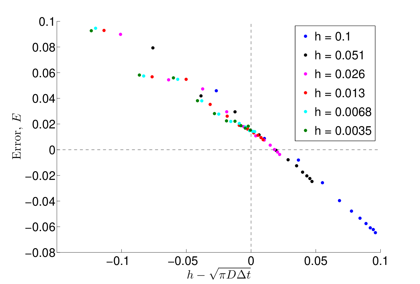Therefore, the error that is due to unphysical shifting of molecules is proportional to the expected shift of molecules as they are transferred from $\Omega_{M}$ to $\Omega_{C}$ . That is $E\propto h_{m}-\sqrt{\pi D\Delta t}$ .

In Figure 5 a dotted red line showing $h_{m}=\sqrt{\pi D\Delta t}$ approximately follows the path of the minimum absolute error. The discrepancy between the actual minimum absolute error and the dotted red line in Figure 5 can be attributed to higher order error that is inherent in the mesoscopic approximation to the diffusion equation. To show that $E\propto h_{m}-\sqrt{\pi D\Delta t}$ , Figure 7 is a plot of error $E$ versus $h_{m}-\sqrt{\pi D\Delta t}$ . The plot is generated by using various values of $h_{m}$ (see legend) and then plotting a number of points while changing $\Delta t$ . Whilst it is clear that the graph is approximately linear, the higher order mesoscopic error is clearly seen in the form of a vertical displacement of this curve about the origin. The effect that the higher order mesoscopic error has on the interface is difficult to quantify because it will depend on the particular molecular system. Therefore, the best choice of parameters that can be chosen for the TRM is $h_{m}\sim\sqrt{\pi D\Delta t}$ .

In Figure 6, we see that the error of the GCM depends on $\Delta t$ and specifically on its relative size compared to $h$ (the analysis of the GCM is provided in A). Rapidly increasing error (quickly saturating the color bar in Figure 6) is observed when $h_{m}\sim\sqrt{\pi D\Delta t}$ . The higher order mesoscopic error artefact can also be seen in Figure 6 since this artefact is independent of the coupling mechanism (see the larger absolute error for large values of $h$ ). The GCM is therefore most accurate for very small values of $\Delta t$ . Whilst in practice making $\Delta t$ small may significantly increase the computing time, small $\Delta t$ is often required for accurate microscopic simulation (for example, capturing reactions with high resolution) and in such cases the GCM is more appropriate than the TRM.

5.2 Three dimensional simulations: CPM versus GCM

In this section we will demonstrate how, when using an unstructured mesh, the error associated with the GCM coupling converges as $\Delta t\rightarrow 0$ whereas error associated with the CPM is minimized when $h\sim\sqrt{D\Delta t}$ where $h$ is the average size of boundary compartments. Both the error associated with the CPM and GCM are due to imbalances in the flux of molecules over the interface. We implement the CPM and GCM in three spatial dimensions using a tetrahedral primal mesh as described in Section 3. The implementation builds on the freely available software URDME [4].

We consider a cube with side length $L=1$ . The cube is first discretized with an unstructured mesh and then divided into a mesoscopic region $\Omega_{\mathrm{C}}$ , and a microscopic region $\Omega_{\mathrm{M}}$ , where $\Omega_{\mathrm{M}}$ is the set of all voxels with a vertex $(x,y,z)$ such that $x<0.5$ and $\Omega_{\mathrm{C}}=\Omega\setminus\Omega_{\mathrm{M}}$ . Here $\Omega$ is the set of all voxels. The partitioning is illustrated in Figure 8 for two different mesh sizes.

We start each simulation with $N_{0}=2\cdot 10^{4}$ molecules whose initial positions are sampled from a uniform distribution. The diffusion constant of the molecules is $D=1$ , and we simulate the system for time t= $0.1$ . Since we start with a uniform distribution and the molecules only diffuse and do not react, we expect the distribution to be uniform at the final time. As the interface is parallel with the $y-z$ -plane, we expect that the distributions of molecules in the $y$ - and $z$ -directions are uniform, but that we get a small error in the distribution of molecules in the $x$ -direction. We now divide the $x$ -axis into $10$ bins of equal length, and then count the number of molecules in each bin at the final time. Mesoscopic molecules are binned by first sampling a continuous position from a uniform distribution on the voxel. We expect $N_{0}/10$ molecules in each bin, and can therefore estimate the error $E$ by

\displaystyle E=\frac{\sum_{i=1}^{10}|N_{i}-N_{0}/10|}{N_{0}}.

(11)

In Figure 9 we have computed $\left\|E\right\|$ for different mesh sizes and time steps. As expected, the error decreases as we refine the mesh and decrease the time step.

In the CPM method, mesoscopic (resp. microscopic) molecules stay mesoscopic (resp. microscopic) during a time step. This implies that the time step should be chosen sufficiently small such that a molecule does not diffuse across several voxels. On the other hand, if the time step is too small the distribution of molecules in space will be biased towards the microscopic region. This can be seen by considering a microscopic molecule diffusing into the mesoscopic regime. If the time step is small, it is likely that it will be close to the microscopic regime at the end of the time step, but if it ends up on the mesoscopic side it will nevertheless be considered uniformly distributed in the voxel at the end of the time step. Thus, the time step should not be chosen too small relative to the size of the voxels, or the error due to the spatial splitting will become large.

Since the GCM converges with decreasing time step, but performs worse for larger time steps, one could suspect that there is a regime where the CPM in [20] performs better than the GCM. At some point, however, the error of the GCM will become small and outperform the CPM in [20]. The errors of the different methods are compared in Figure 10 for a mesh with $49101$ voxels. Indeed, we see that the CPM method performs better for time steps down to almost $\Delta t=10^{-4}$ , at which point the error of the GCM method becomes smaller.

6 Summary

In this paper we have compared two existing mesoscopic-microscopic coupling techniques for stochastic simulations of reaction-diffusion processes with a new convergent method called the ghost cell method (GCM). Here we will summarize the specific sources of error of the TRM, CPM and GCM, when they converge, how they may be optimized for accuracy and notes on their computational efficiency.

6.1 Summary of the two-regime method

The TRM couples molecules by considering that mesoscopic compartments contain molecules that are evenly distributed in a probabilistic sense. As these molecules diffuse over the interface they are placed according to the distribution $f(x)$ given by (7). Molecules migrating in reverse from the microscopic regime to the mesoscopic regime must be absorbed by the interfacial compartments and be indistinguishable from other molecules in these compartments by virtue of this paradigm. As such, instead of migrating an average distance over the interface proportional to $\sqrt{\Delta t}$ it becomes evenly distributed over the compartment with an expected location of $h/2$ over the interface. The molecules are therefore effectively shifted $(h-\sqrt{\pi D\Delta t})/2$ into the compartment regime. This shift in the molecules therefore creates a discontinuity of in the distribution to find molecules on the interface and therefore an error due to the presence of the coupling proportional to $h-\sqrt{\pi D\Delta t}$ . The nature of this error is that, if the expected net flux of molecules over the interface is 0, then no error due to the presence of the interface will be experienced. This is important to note, since, this is not the case for both the CPM and GCM methods. Furthermore, since the error is proportional to $h-\sqrt{\pi D\Delta t}$ it clearly converges in the limiting case (ii) described in the introduction but not in the limiting case (i).

Whilst the TRM can give controllably accurate results, it can be computationally more costly to implement. This is because perfect absorption of molecules is required on the boundary and this means that each molecule in the molecular-based domain needs to be checked for interaction with the boundary in a given time step using (3).

6.2 Summary of the compartment-placement method

The CPM is a coupling mechanism that, whilst heuristically derived, can produce accurate results under some circumstances and do so with minimum computational cost. Molecules are placed within a pseudo-compartment in the molecular-based domain via diffusion from the compartment-based domain. In reverse molecules are placed in compartments from the molecular-based domain via diffusion of these molecules in the continuous domain over the interface. The antisymmetry that is seen in the methods of migration, mesoscopic to microscopic and microscopic to mesoscopic, result in a boundary layer in the expected distribution of molecules at the interface. This boundary layer is caused by the fact that molecules diffusing from the molecular region to the compartmental region are considered uniformly distributed on the compartment at the end of the time step. If $\Delta t$ is small compared to $h$ , this will be a poor approximation. It should thus be noted that the error of the CPM does not converge in the limiting case (i) described in the introduction, however the error appears to converge according to limiting case (ii).

The CPM is computationally efficient. Its only inefficiency is that, unlike the TRM, it requires the knowledge of a pseudo-compartment in the microscopic domain. The TRM is therefore more appropriate than the CPM for coupling completely independent simulation algorithms, since the CPM requires its own custom algorithm to be implemented fully.

6.3 Summary of the ghost cell method

The GCM couples molecules according to a discrete domain on each side of the interface. Molecules that are in the microscopic domain are binned according to a ghost compartment/cell and jump into the mesoscopic domain using jump rates derived using the mesoscopic approach. In such a way, symmetry is conserved in the method of migration from mesoscopic to microscopic and from microscopic to mesoscopic, unlike the CPM. It is important that the molecules are binned correctly for this coupling to work accurately. The error, therefore, can be attributed to molecules that are in the ghost cell when they should not be, or not in the ghost cell when they should be. Therefore, if the compartment size $h$ at the interface (and of the ghost cell) is much larger than the resolution of the particle tracking in the microscopic domain, the correct number of molecules will be in the ghost cell. The error therefore converges in the limit of small $\Delta t$ so long as $h$ is sufficiently coarse. Furthermore, it is possible to show that, unlike the TRM, this source of error is not due to a displacement of molecules but an unballanced flux of molecules (see A) and will therefore appear even if the expected net flux over the interface is 0. The GCM, however, is convergent in the limiting case (i) but not (ii) from the introduction giving the GCM a unique advantage over both the CPM and TRM.

The GCM is computationally efficient for small $\Delta t$ since the jump rates from the microscopic domain to the mesoscopic domain are determined by the ghost cell size and not the time step (like the TRM for example).

Acknowledgements: The research leading to these results has received funding from the European Research Council under the European Community’s Seventh Framework Programme (FP7/2007-2013)/ ERC grant agreement No. 239870. This publication was based on work supported in part by Award No KUK-C1-013-04, made by King Abdullah University of Science and Technology (KAUST). Stefan Hellander has been supported by the National Institute of Health under Award no. 1R01EB014877-01 and the Swedish Research Council. Radek Erban would also like to thank Brasenose College, University of Oxford, for a Nicholas Kurti Junior Fellowship; the Royal Society for a University Research Fellowship; and the Leverhulme Trust for a Philip Leverhulme Prize.

Appendix A Mathematical justification for the ghost cell method

Here we present an analysis of the GCM in one-dimension. We show that error of the GCM that is produced on the interface between mesoscopic and microscopic subdomains converges in the case (i). Specifically, we see convergence of the interface-derived error as $\Lambda=\sqrt{D\Delta t}/h\rightarrow 0$ . This property of convergence is unique to the GCM when compared with other reported coupling mechanisms. In showing that the interface-derived error vanishes in the small time step limit, we will show that rapid variation within the boundary layer of the interface vanishes as $\Lambda\rightarrow 0$ , leaving behind a linear approximation of the true distribution of molecules. Since the error at the interface will be of order $h^{2}$ it is accurate to the same order as the mesoscopic algorithm itself.

Without loss of generality, consider an interface at $x=0$ on an infinite one-dimensional domain. To the left of this interface ( $x<0$ ) a compartment-based model is used with fixed compartment size $h$ . To the right of the interface ( $x>0$ ) a molecular-based algorithm is used and is updated at fixed time increments of $\Delta t$ , i.e. $\Omega_{C}=(-\infty,0)$ and $\Omega_{M}=(0,\infty)$ . We denote the compartments in $\Omega_{C}$ by $C_{k}=(-kh,-kh+h)$ , where $k=1,2,\dots.$ Then the interface compartment is $C_{1}=(-h,0)$ . The ghost cell will be denoted by $C_{M}=(0,h)$ .

Molecules in $\Omega_{C}$ are described only by their compartment. Their compartment changes with an exponentially distributed random time with a rate that is given by $D/h^{2}$ . This rate is conditional on initial and final states being compartments. The rate given by $D/h^{2}$ is chosen in such a way that the expected number of molecules in each compartment matches that of a discretized diffusion equation (see (4) and (5)). These rates, however, breakdown in the case of the TRM because the initial and final states of jump across the interface are not compartments but rather the final state is a molecule in $\Omega_{M}$ . The jump across the boundary for the TRM is given by (6). Molecules in $\Omega_{M}$ have one thing in common with those in compartments. A domain that is modeled microscopically and then binned into compartments shows the same expected behaviour as a domain modeled with compartments to leading and first order accuracy in $h$ in the limit as $\Delta t\rightarrow 0$ . Therefore, in an attempt to interface the two regimes together it may be appropriate to bin molecules in $\Omega_{M}$ into a ghost cell/compartment $C_{M}$ near the interface. The molecules that are in $C_{M}$ will then have the same properties as a compartment from the perspective of the interface compartment $C_{1}$ . To this end, any molecule in $C_{M}$ may spontaneously change state from the molecular domain to $C_{1}$ . We expect that since the interface compartment-bound molecules see a compartment state for molecules in $C_{M}$ , the change of state from $C_{1}$ to a random position within $C_{M}$ will occur with a normal inter-compartmental rate. In the following analysis we show that this is the case.

We shall test the hypothesis by matching the master equations for $C_{1}$ and the probability distribution in $\Omega_{M}$ in such a way that no rapid variation in probability to find molecules, $\bar{p}(x,t)$ , is apparent at the interface. We shall assume that the rate for molecules to jump into $\Omega_{M}$ from $C_{1}$ is $\Gamma^{+}$ and are placed in an initial position from the interface given by the probability distribution $f(x)$ . Molecules in $\Omega_{M}$ spontaneously jump into $C_{1}$ with a rate $\Gamma^{-}g(x)$ . Functions $f(x)$ and $g(x)$ are normalized such that they have a unit integral over $\Omega_{M}$ . We shall show that

\Gamma^{+}=\Gamma^{-}=\frac{D}{h^{2}}\qquad\mbox{and}\qquad g(x)=f(x)=\left\{\begin{matrix}\displaystyle\frac{1}{h},&\mbox{for}\;x\in C_{M};\\ \rule{0.0pt}{14.22636pt}0,&\mbox{otherwise.}\end{matrix}\right.

(12)

We will find it convenient for the sake of notation to introduce the parameters

\alpha^{\pm}=\frac{h^{2}\Gamma^{\pm}}{D},\qquad\mbox{and}\qquad\Lambda=\frac{\sqrt{D\Delta t}}{h}.

To show (12) we focus on the purely diffusive problem, since bulk reactions have no effect on boundary conditions. In order to limit the flux of molecules jumping into $C_{1}$ , all molecules in $\Omega_{M}$ that hit the interface by Brownian motion are reflected back to $\Omega_{M}$ .

We denote the probability of finding a molecule in compartment $C_{k}$ , $k=1,2,\dots,$ by $p_{k}(t)h$ (so that $p_{k}(t)$ approximates the probability density function at the node within this compartment). If we denote by $p(x,t)$ the probability density function of the discrete-time molecular-based algorithm, then the transmission/reflection rules give us the following master equation

$\displaystyle p_{1}(t+\Delta t)$	$\displaystyle=$	$\displaystyle\left(1-(1+\alpha^{+})\Lambda^{2}\right)p_{1}(t)+\Lambda^{2}\,p_{2}(t)+\alpha^{-}\Lambda^{2}\int_{0}^{\infty}g(x)p(x,t)\,\mbox{d}x,\qquad$	(13)
$\displaystyle p(x,t+\Delta t)$	$\displaystyle=$	$\displaystyle\int_{0}^{\infty}\frac{p(y,t)}{\sqrt{4\pi D\Delta t}}\left[\exp\left(\frac{-(x-y)^{2}}{4D\Delta t}\right)+\exp\left(\frac{-(x+y)^{2}}{4D\Delta t}\right)\right]\,\mbox{d}y$	(14)
		$\displaystyle\mbox{ }+\frac{\alpha^{+}D\Delta tp_{1}(t)f(x)}{h}-\frac{\alpha^{-}D\Delta tp(x,t)g(x)}{h}.$	(14)

In the vicinity of $x=0$ there is a boundary layer of width $O(h)$ so long as $f(x)$ and $g(x)$ vanish for $x\gg h$ [6]. We rescale (13) and (14) using the (dimensionless) boundary layer coordinate $\xi=x/h$ . We also denote $p_{\mathrm{inner}}(\xi,t)=p(h\xi,t)$ , $f_{\mathrm{inner}}(\xi)=h\,f(h\xi)$ and $g_{\mathrm{inner}}(\xi)=h\,g(h\xi)$ . The rescalings of $f$ and $g$ by $h$ are done to keep the integrals of these functions equal to 1. Thus, in the boundary layer coordinates, (13) and (14) become

$\displaystyle p_{1}(t+\Delta t)$	$\displaystyle=$	$\displaystyle\left(1-(1+\alpha^{+})\Lambda^{2}\right)p_{1}(t)+\Lambda^{2}p_{2}(t)$	(15)
		$\displaystyle\mbox{ }+\alpha^{-}\Lambda^{2}\int_{0}^{\infty}g_{\mathrm{inner}}(\xi)\,p_{\mathrm{inner}}(\xi,t)\,\mbox{d}\xi,$	(15)
$\displaystyle p_{\mathrm{inner}}(\xi,t+\Delta t)$	$\displaystyle=$	$\displaystyle\Lambda^{-1}\int_{0}^{\infty}p_{\mathrm{inner}}(\eta,t)\left[K\left(\Lambda^{-1}(\eta-\xi)\right)+K\left(\Lambda^{-1}(\eta+\xi)\right)\right]\,\mbox{d}\eta$	(16)
		$\displaystyle\mbox{ }+\alpha^{+}\Lambda^{2}p_{1}(t)\,f_{\mathrm{inner}}(\xi)-\alpha^{-}\Lambda^{2}p_{\mathrm{inner}}(\xi,t)\,g_{\mathrm{inner}}(\xi),$	(16)

where $K(x)=(4\pi)^{-1/2}\exp(-x^{2}/4)$ . The parameter $\Lambda$ gives us the relative size of $D\Delta t$ to $h^{2}$ and we wish to show that as $\Lambda\rightarrow 0$ the distribution of molecules across the boundary is smooth and the error that remains is of the order of $h^{2}$ , which is the same size of the error associated with the mesoscopic discretization in $\Omega_{C}$ . In order to join these models smoothly we require in $\Omega_{C}$ that

$\displaystyle p_{1}(t)$	$\displaystyle=$	$\displaystyle p(-h/2,t)=p(0,t)-\frac{h}{2}\bar{p}_{x}(0,t)+O(h^{2})+O(\Lambda),$	(17)
$\displaystyle p_{2}(t)$	$\displaystyle=$	$\displaystyle p(-3h/2,t)=p(0,t)-\frac{3h}{2}\bar{p}_{x}(0,t)+O(h^{2})+O(\Lambda),$	(18)
$\displaystyle p_{1}(t+\Delta t)$	$\displaystyle=$	$\displaystyle p_{1}(t)+O(\Delta t),$	(19)

while, for the molecular-based side, we want variation from the linear approximation in the boundary layer to be limited to $O(\Lambda)$ up to order $h^{2}$ accuracy, so that

	$\displaystyle p_{\mathrm{inner}}(\xi,t)$	$\displaystyle=$	$\displaystyle p(0,t)+h\,\xi\,p_{x}(0,t)+O(h^{2})+O(\Lambda),$		(20)
	$\displaystyle p_{\mathrm{inner}}(\xi,t+\Delta t)$	$\displaystyle=$	$\displaystyle p_{\mathrm{inner}}(\xi,t)+O(\Delta t).$		(21)

The prescription of a consistent probability density $p(0,t)$ and derivative $p_{x}(0,t)$ for both sides of the interface, along with linear approximations sufficiently close to the interface equates to continuity and differentiability over the interface which is the matching condition that we are attempting to achieve.

Substituting (17)–(21) into (15) and (16) and equating terms of the same order in $h$ and leading order in $\Lambda$ gives the following conditions that must be placed on $g(x)$ , $f(x)$ , $\alpha^{+}$ and $\alpha^{-}$ :

(i) $O(h^{0}\Lambda^{0})$ terms from equation (15) give condition:

\alpha^{+}=\alpha^{-}\int_{0}^{\infty}g_{\mathrm{inner}}(\xi),\mbox{d}\xi.

(22)

Condition (22) states how the relative rates for molecules to transition to and from $\Omega_{M}$ and $\Omega_{C}$ must be dependent on the relative sizes of $C_{1}$ and $C_{M}$ .

(ii) $O(h^{1}\Lambda^{0})$ terms from equation (15) give condition:

2=\alpha^{+}+\alpha^{-}\int_{0}^{\infty}\xi g_{\mathrm{inner}}(\xi),\mbox{d}\xi.

(23)

Condition (23) states how the rates for molecules to transition to and from $\Omega_{M}$ and $\Omega_{C}$ depend on the average distance molecules are placed from the interface when placed within $C_{M}$ . This is the same condition given in $\Omega_{C}$ for jumps between the compartments.

(iii) $O(h^{0}\Lambda^{0})$ terms from equation (16) give condition:

\alpha^{+}f_{\mathrm{inner}}(\xi)=\alpha^{-}g_{\mathrm{inner}}(\xi).

(24)

Condition (24) states that molecules must be placed into $\Omega_{M}$ with the same probability weighting that they are taken out and placed back into $\Omega_{C}$ .

(iv) $O(h^{1}\Lambda^{0})$ terms from equation (16) are automatically satisfied.

The GCM that is presented in this manuscript uses parameters (12) which satisfy the three conditions (22)–(24) listed above. Such a scheme, therefore, has an error that is no greater than the error of the mesoscopic scheme in the limit $\Lambda\rightarrow 0$ , in other words, in the limit $\Delta t\rightarrow 0$ whilst $h$ remains constant.

References

[1] B. Alberts, A. Johnson, J. Lewis, M. Raff, K. Roberts, and P. Walter. Molecular Biology of the Cell. Garland Science, New York, 2007.
[2] F. Alexander, A. Garcia, and D. Tartakovsky. Algorithm refinement for stochastic partial differential equations: I. linear diffusion. Journal of Computational Physics, 182(1):47–66, 2002.
[3] S. Andrews and D. Bray. Stochastic simulation of chemical reactions with spatial resolution and single molecule detail. Physical Biology, 1:137–151, 2004.
[4] B. Drawert, S. Engblom, and A. Hellander. URDME: A modular framework for stochastic simulation of reaction-transport processes in complex geometries. BMC Syst. Biol., 6:76, 2012.
[5] S. Engblom, L. Ferm, A. Hellander, and P. Lötstedt. Simulation of stochastic reaction-diffusion processes on unstructured meshes. SIAM Journal on Scientific Computing, 31:1774–1797, 2009.
[6] R. Erban and S. J. Chapman. Reactive boundary conditions for stochastic simulations of reaction-diffusion processes. Physical Biology, 4(1):16–28, 2007.
[7] R. Erban and S. J. Chapman. Stochastic modelling of reaction-diffusion processes: algorithms for bimolecular reactions. Physical Biology, 6(4):046001, 2009.
[8] R. Erban, S. J. Chapman, and P. Maini. A practical guide to stochastic simulations of reaction-diffusion processes. 35 pages, available as http://arxiv.org/abs/0704.1908, 2007.
[9] R. Erban, M. Flegg, and G. Papoian. Multiscale stochastic reaction-diffusion modelling: application to actin dynamics in filopodia. to appear in the Bulletin of Mathematical Biology, 2013.
[10] M. Flegg, J. Chapman, and R. Erban. The two-regime method for optimizing stochastic reaction-diffusion simulations. Journal of the Royal Society Interface, 9(70):859–868, 2012.
[11] M. Flegg, J. Chapman, L. Zheng, and R. Erban. Analysis of the two-regime method on square meshes. submitted to SIAM Journal on Scientific Computing, 23 pages, available as http://arxiv.org/abs/1304.5487 2013.
[12] M. Flegg, S. Rüdiger, and R. Erban. Diffusive spatio-temporal noise in a first-passage time model for intracellular calcium release. to appear in the Journal of Chemical Physics, 2013.
[13] E. Flekkøy, J. Feder, and G. Wagner. Coupling particles and fields in a diffusive hybrid model. Physical Review E, 64:066302, 2001.
[14] B. Franz, M. Flegg, J. Chapman, and R. Erban. Multiscale reaction-diffusion algorithms: PDE-assisted Brownian dynamics. available as http://arxiv.org/abs/1206.5860, to appear in SIAM Journal on Applied Mathematics, 2013.
[15] T. Geyer, C. Gorba, and V. Helms. Interfacing Brownian dynamics simulations. Journal of Chemical Physics, 120(10):4573–4580, 2004.
[16] M. Gibson and J. Bruck. Efficient exact stochastic simulation of chemical systems with many species and many channels. Journal of Physical Chemistry A, 104:1876–1889, 2000.
[17] D. Gillespie. Exact stochastic simulation of coupled chemical reactions. Journal of Physical Chemistry, 81(25):2340–2361, 1977.
[18] C. Gorba, T. Geyer, and V. Helms. Brownian dynamics simulations of simplified cytochrome c molecules in the presence of a charged surface. Journal of Chemical Physics, 121(1):457–464, 2004.
[19] J. Hattne, D. Fange, and J. Elf. Stochastic reaction-diffusion simulation with MesoRD. Bioinformatics, 21(12):2923–2924, 2005.
[20] A. Hellander, S. Hellander, and P. Lötstedt. Coupled mesoscopic and microscopic simulation of stochastic reaction-diffusion processes in mixed dimensions. Multiscale Modeling and Simulation, 10(2):585–611, 2012.
[21] M. Klann, A. Ganguly, and H. Koeppl. Hybrid spatial Gillespie and particle tracking simulation. Bioinformatics, 28(18):i549–i555, 2012.
[22] J. Lipkova, K. Zygalakis, J. Chapman, and R. Erban. Analysis of Brownian dynamics simulations of reversible bimolecular reactions. SIAM Journal on Applied Mathematics, 71(3):714–730, 2011.
[23] E. Moro. Hybrid method for simulating front propagation in reaction-diffusion systems. Physical Review E, 69:060101, 2004.
[24] S.A. Rice. Diffusion Limited Reactions. Amsterdam: Elsevier, 1 edition, 1985.
[25] J. van Zon and P. ten Wolde. Green’s-function reaction dynamics: a particle-based approach for simulating biochemical networks in time and space. Journal of Chemical Physics, 123:234910, 2005.
[26] G. Wagner and E. Flekkøy. Hybrid computations with flux exchange. Philosophical Transactions of the Royal Society A: Mathematical, Physical & Engineering Sciences, 362:1655–1665, 2004.