Statistics of Avalanches with Relaxation, and Barkhausen Noise: A Solvable ModelThanks: LPTENS is a Unité Propre du C.N.R.S. associée à l’Ecole Normale Supérieure et à l’Université Paris Sud
Abstract
We study a generalization of the Alessandro-Beatrice-Bertotti-Montorsi (ABBM) model of a particle in a Brownian force landscape, including retardation effects. We show that under monotonous driving the particle moves forward at all times, as it does in absence of retardation (Middleton’s theorem). This remarkable property allows us to develop an analytical treatment. The model with an exponentially decaying memory kernel is realized in Barkhausen experiments with eddy-current relaxation, and has previously been shown numerically to account for the experimentally observed asymmetry of Barkhausen-pulse shapes. We elucidate another qualitatively new feature: the breakup of each avalanche of the standard ABBM model into a cluster of sub-avalanches, sharply delimited for slow relaxation under quasi-static driving. These conditions are typical for earthquake dynamics. With relaxation and aftershock clustering, the present model includes important ingredients for an effective description of earthquakes. We analyze quantitatively the limits of slow and fast relaxation for stationary driving with velocity . The -dependent power-law exponent for small velocities, and the critical driving velocity at which the particle velocity never vanishes, are modified. We also analyze non-stationary avalanches following a step in the driving magnetic field. Analytically, we obtain the mean avalanche shape at fixed size, the duration distribution of the first sub-avalanche, and the time dependence of the mean velocity. We propose to study these observables in experiments, allowing to directly measure the shape of the memory kernel, and to trace eddy current relaxation in Barkhausen noise.
pacs
02.50.Ey, 05.40.Jc, 75.60.EjI Introduction and model
I.1 Barkhausen noise
The Barkhausen noise [1] is a characteristic magnetic signal emitted when a soft magnet is slowly magnetized. It can be measured and made audible as crackling through an induction coil: periods of quiescence followed by pulses, or avalanches, of random strength and duration. The statistics of the emitted signal depends on material properties and its state. By analyzing the Barkhausen signal, one can deduce for example residual stresses [2, 3] or grain sizes [4, 5] in metallic materials. Understanding how particular details of the Barkhausen noise statistics depend on microscopic material properties is important for such applications.
On the other hand, Barkhausen noise pulses are just one example for avalanches in disordered media. Such avalanches also occur in the propagation of cracks during fracture [6, 7, 8], in the motion of fluid contact lines on a rough surface [9, 10, 11, 12], and as earthquakes driven by motion of tectonic plates [13, 14, 15, 16]. Some features of the avalanche statistics, like size and duration distributions [17, 18], are universal for many of these phenomena [19]. Barkhausen noise is easily measurable experimentally, and provides a good way to study aspects of avalanche dynamics common to all these systems.
A first advance in the theoretical description of Barkhausen noise was the stochastic model postulated by Alessandro, Beatrice, Bertotti and Montorsi [20, 21] (ABBM model). They proposed modeling the domain-wall position through the stochastic differential equation (SDE)
| (1) |
We follow here the conventions of [22] and [23]. is the saturation magnetization, and the external field which drives the domain-wall motion. A typical choice is a constant ramp rate , , which leads to a constant average domain-wall velocity [20]. is the demagnetizing factor characterizing the strength of the demagnetizing field generated by effective free magnetic charges on the sample boundary [20, 24]. The domain-wall motion induces a voltage proportional to its velocity , which is the measured Barkhausen noise signal. Here is a random local pinning force. It is assumed to be a Brownian motion, i.e. Gaussian with correlations
This choice may seem unnatural, since the physical disorder does not exhibit such long-range correlations. It is only recently that it has been shown [25, 17, 18] that the “ABBM guess” emerges as an effective disorder to describe the avalanche motion of the center-of-mass of the interface, denoted , in the mean-field limit of the field theory of an elastic interface with internal dimensions. This correspondence holds both for interfaces driven quasi-statically [25, 18], and for static interfaces at zero temperature [17]. The mean-field description is accurate above a certain critical internal dimension . For , a systematic expansion in using the functional renormalization group yields universal corrections to the scaling exponents [26, 27, 28] and avalanche size [17, 18] and duration [25, 29, 18] distributions.
For the particular case of magnetic domain walls, the predictions of the ABBM model are well verified experimentally in certain ferromagnetic materials, for example FeSi alloys [21, 30, 31]. These are characterized by long-range dipolar forces decaying as between parts of the domain wall a distance apart. This leads [32] to a critical dimension coinciding with the physical dimension of the domain wall. In this kind of systems, as expected, the mean-field approximation is reasonably well satisfied. Measurements on other types of ferromagnets, for example FeCoB alloys [31] indicate a universality class different from the mean-field ABBM model. This may be explained by short-range elasticity, and a critical dimension . To describe even the center of mass mode in this class of domain walls, one needs to take into account the spatial structure of the domain wall. Predictions for roughness exponents [27, 28] and avalanche statistics [25, 29, 17, 18] for this non-mean-field universality class have been obtained using the functional renormalization group.
On the other hand, even for magnets in the mean-field universality class, a careful measurement of Barkhausen pulse shapes [33, 34, 19, 22] shows that they differ from the simple symmetric shape predicted by the ABBM model [35, 25]. This hints at a more complicated equation of motion than the first-order overdamped dynamics usually considered for elastic interfaces in disordered media.
In a physical interface, there may be additional degrees of freedom. One example was studied in [36, 37]. Other examples include deformations of a plastic medium, or eddy currents arising during the motion of a magnetic domain wall. For viscoelastic media, these can be modeled by a memory term which is non-local in time [38, 39]. At mean-field level, this is equivalent to a model with dynamical stress overshoots [40]. Such memory terms may lead to interesting new phenomena, like coexistence of pinned and moving states [38, 39, 41]. A similar memory term, non-local in time, is argued in [22] to describe the dissipation of eddy currents in magnetic domain-wall dynamics,
| (2) |
The response function , derived by solving the Maxwell equations in a rectangular sample [42, 22, 23, 24], is
| (3) |
are relaxation times for the individual eddy current modes,
They depend on the sample width , thickness , permeability and conductivity . (2) and (3) correspond to Eqs. (13), (17) and (21) in [23]; we refer the reader there for details of the derivation.
Zapperi et al. [22] showed numerically that avalanche shapes in the model (2) are asymmetric. They concluded that eddy-current relaxation may be one way of explaining the experimentally observed skewness of Barkhausen noise pulses. They also argue that similar relaxation effects may be relevant for other physical situations where asymmetric pulse shapes are observed11 1 For example, [22] mentions slip velocity profiles during earthquakes [43, 14]. However, it is not clear if there are physical reasons to expect a relaxation of the form (2)..
A simplification of Eq. (3) occurs when considering only the leading contributions for small and large relaxation times22 2 We have and . Thus, for small times, is well approximated by for some constant . On the other hand, for long times, only the mode that relaxes slowest remains. Hence, for long times one can set . . Then one obtains [22] a natural generalization of the ABBM equation (1):
| (4) |
Here, is the longest relaxation time of the eddy-current modes, . and are damping coefficients given in [22].
I.2 The ABBM model with retardation
For the remainder of this work, we adopt the conventions used in the study of elastic interfaces. Let us introduce a more general model than (4),
| (5) |
which describes a particle driven in a force landscape , with retardation. At this stage is arbitrary. Here is a general memory kernel with the following properties:
- 1.
(without loss of generality, since a constant may be absorbed into the parameter ).
- 2.
as .
- 3.
for all , i.e. memory of the past trajectory always decays with time.
This model possesses a remarkable property for any such kernel and any landscape . It has monotonicity, i.e. it satisfies the Middleton theorem: For non-negative driving , after an initial transient period one has at all times. A more precise statement and a proof are given in Appendix A. It has very important consequences, both in the driven regime, and in the limit of quasi-static driving, i.e. small . In that limit it converges to the quasi-static process , where is the (forward) Middleton metastable state, defined as the smallest (leftmost) root of
| (6) |
It is independent of the precise form of the kernel . Hence the domain-wall position is uniquely determined by the value of the driving field , due to the monotonicity property [44]. This process exhibits jumps at a set of individual points, the avalanche locations , and the quasi-static avalanche sizes
| (7) |
are thus independent of the retardation kernel. What depends on the kernel is the dynamics within these avalanches, and that is studied here. The quasi-static avalanche sizes have a well-defined distribution which has been computed for a particle in various force landscapes [45, 46] and for the non-trivial case of a -dimensional elastic interface using functional RG methods [29, 47, 48]. As long as the dynamics obeys the Middleton theorem, the avalanche-size distribution remains independent of the details of the dynamics [18].
While monotonicity holds for any , in this article we focus on the case of the Brownian force landscape which can be solved analytically. As in the standard ABBM model, we choose the effective random pinning force to be a random walk, i.e. Gaussian with correlator given by (I.1). 33 3 It can be realized as a stationary landscape, with a cutoff at scale , or by (non-stationary landscape with ). In both cases is a white noise, and that is the important feature. We call this the ABBM model with retardation. In view of the application to Barkhausen noise, the parameter describes the overall strength of the force exerted by eddy currents on the domain wall. For , (5) reduces to the equation of the standard ABBM model in the conventions of [45, 46].
The retarded ABBM model is particularly interesting in view of the monotonicity property. Other ways of generalizing the ABBM model to include inertia, e.g. by a second-order derivative [49], do not inherit this property from the standard ABBM model. This makes the ABBM model with retardation very special, and it will be important for its solution in section III.
When considering the particularly interesting case of exponential relaxation motivated in [22], we set
| (8) |
is the longest time scale of eddy-current relaxation, as discussed above. In this approximation, (5) can be re-written as two coupled, local equations for the domain-wall velocity , and the eddy-current pressure ,
| (9) | ||||
| (10) | ||||
| (11) |
Although most of our quantitative results will be derived for this special case only, most qualitative features carry over to more general kernels with sufficiently fast decay.
By rescaling , and in Eq. (5) (for details, see section III.1), one finds the characteristic time scale and length scale of the standard ABBM model (). They set the scales for the durations and sizes of the largest avalanches. There are of course avalanches of smaller size (up to some microscopic cutoff if one defines it). The velocity scale is and one can define a renewal time for the large avalanches as , the limit of quasi-static driving being , equivalent to . In the retarded ABBM model (8) one introduces an additional memory time scale and various regimes will emerge depending on how compares with the other time scales (whose meaning will be changed).
Eq. (11) then describes a depinning model with relaxation, i.e. one can think of the disorder landscape as relaxing via the additional degree of freedom . This is a feature of interest for earthquake models as discussed below. In this context one considers the limit of well separated time scales, .
Other features of Barkhausen noise predicted for the ABBM model with retardation are quite different from those of the standard ABBM model. Zapperi et al. [22] already realized that the inclusion of eddy currents leads to a skewness in the avalanche shape. In this article, we go further and discuss changes in the avalanche statistics. The relaxation of eddy currents introduces an additional slow time scale into the model. This leads to avalanches which stretch further in time. In particular, avalanches following a kick (or, more generally, stopped driving) never terminate, by contrast with the standard ABBM model. This is because of the exponentially decaying retardation kernel, which never vanishes 44 4 For a model such that for , avalanches would remain of finite duration.. Avalanche sizes however, are not changed by retardation in the limit of quasi-static driving, as discussed above. In that limit, retardation leads to a break-up of avalanches into sub-avalanches, which can also be called aftershocks. Avalanches at continuous driving overlap stronger, and the velocity threshold for the infinite avalanche (i.e. the velocity no longer vanishes) is decreased. We now describe these effects in detail and formulate more precise statements.
I.3 Protocols
Let us first review qualitatively the main situations that we will study, and define the terminology.
(i) stationary driving: The driving velocity is constant, , and the distributions of the domain-wall velocity and of the eddy-current pressure reach a steady state, which we study. If is large enough the velocity will never vanish and one has a single infinite avalanche, also called “continuous motion”. At smaller the velocity will sometimes vanish. That defines steady state avalanches. These are more properly called sub-avalanches of the infinite avalanche since at finite they immediately restart. Only in the limit they become well separated in time and can then be called steady state avalanches.
(ii) Avalanches following a kick: We consider an initial condition at prepared to lie in the “Middleton attractor” at , as discussed above. It can be obtained by driving the system monotonously in the far past with , until memory of the initial condition is erased; then let it relax for a long time with until time . Hence the initial condition is . At one changes the external magnetic field instantaneously by , i.e. sets . For , the external field does not change anymore, thus a kick in the driving velocity corresponds to a step in the applied force. At the system has settled again into the Middleton attractor at because of the properties discussed above. One can thus consider the total motion to define a single avalanche following a kick, which is thus unambiguously defined. The total size is the same as in the absence of retardation. We will ask about the total duration (which becomes infinite) and whether the velocity has vanished at intermediate times, i.e. whether the avalanche has broken into sub-avalanches.
Avalanches following a kick are called non-stationary avalanches (since driving is non-stationary). However, in the limit of they become identical to the steady-state avalanches obtained by stationary driving discussed above (conditioned to start at ).
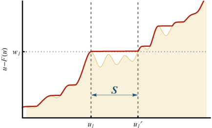
(a) Standard ABBM model.
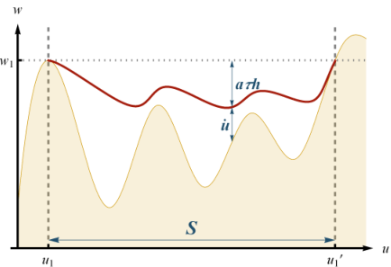 (b) ABBM model with retardation, .
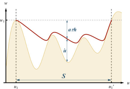 (c) ABBM model with retardation, .
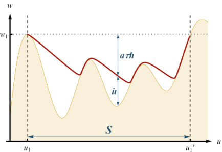 (d) ABBM model with retardation, .
I.4 Organization of this article
The remainder of this article is structured as follows: In section II, we discuss in more detail the phenomenology and the qualitative physics of the ABBM model with retardation. We discuss the splitting of a quasi-static avalanche into sub-avalanches, and the effects of retardation on the stationary and the non-stationary dynamics.
In section III we explain how the probability distribution of observables linear in the domain-wall velocity can be computed by solving a non-linear, non-local “instanton” equation. By this, the stochastic model is mapped onto a purely deterministic problem of non-linear dynamics. This is a generalization of the method developed in [25, 46] for the standard ABBM model with arbitrary driving.
Section IV discusses how the explicit form of the memory kernel can be extracted in an experiment from the response to a kick.
Section V is devoted to an analysis of the instanton equations in the limit . This means that eddy currents relax much more slowly than the domain wall moves. In this limit, we obtain the stationary distributions of the eddy-current pressure and domain-wall velocity, as well as their behavior following an instantaneous kick in the driving field. The instanton solution reflects the two time scales in the problem: A short time scale, on which eddy currents build up but do not affect the dynamics, and a long time scale, on which they relax quasi-statically. We prove that, even after the driving has stopped, the velocity never becomes zero permanently.
In section VI we discuss the fast-relaxation limit . In this limit, eddy currents relax much faster than the domain wall moves. The instanton solutions again exhibit two time scales, but now eddy currents are irrelevant for the long-time asymptotics. Qualitative results (like the fact that the domain-wall motion never stops entirely) are in agreement with those for the slow-relaxation limit, considered in section V.
In section VII we discuss non-stationary avalanches following an instantaneous kick in the driving. In particular, we compute their average shape at fixed size.
In section VIII, we show how to include an absorbing boundary in the instanton solution of section III. This is required for treating avalanches during stationary driving. We then derive the distribution of avalanche durations in the standard ABBM model at finite driving velocity, , and the leading corrections for weak relaxation and . We also show numerical results for more general situations, and give some conjectures on the modification of size and duration exponents by retardation effects.
Last, in section IX, we summarize our results. We discuss how they can be used to learn more about the dependence of Barkhausen noise on eddy current dissipation.
II Physics of the model and summary of the results
II.1 Quasi-static driving: Sub-avalanches and aftershocks
Consider the system either under stationary driving at , or following an infinitesimal kick as discussed above, and call the starting time of the avalanche. The main physics can be understood from figure 1 and keeping in mind the equations (11).
In Fig. 1a we represent the usual construction for in the standard ABBM as the left-most solution of the equation (6) (in the figure we set ). Assuming this construction indicates the position of the domain wall as a function of on time scales of order . At the solution jumps from to corresponding to an avalanche of size ; the latter occurs on the much faster time scale . During the avalanche the velocity (setting ) is given by the difference in height between the line and the landscape , providing a graphic representation of the motion. The velocity vanishes at and . For illustration we have represented a force landscape which is ABBM like at large scales but smooth at small scales. For the continuous ABBM model the construction is repeated at all scales and one has avalanches of all smaller sizes.
Let us now add retardation, setting , and varying the memory time . The graphical construction corresponding to Eq. (11) is represented in Fig. 1b to 1d. The difference in height is now the sum of and (in the Figure we chose ), which evolves according to the second equation in Eq. (11). It can be rewritten as
| (12) |
Hence increases from , initially as (since ). Thus the curve versus starts with a negative slope .
Another way to see this is to note that for , the second equation of (11) gives
| (13) |
Inserting this into the first equation of (11), we obtain
| (14) |
Effectively, for short times the mass is modified from . Thus, while is fixed, the end of the first sub-avalanche is determined not by the roots of , but by the roots of . Equivalently, in the landscape , instead of looking at intersections with the horizontal curve , we should look at intersections with , a line with slope .
At the point where this curve intersects first the landscape we get a point where first vanishes. This defines the size of the first sub-avalanche. If is small this usually occurs near the end, but if is larger the original avalanche (called main avalanche) is divided – in size – in a sequence of sub-avalanches . The number of sub-avalanches in the main avalanche is finite for a smooth landscape, and infinite for the continuous Brownian landscape. The total size is however the same as for , due to the Middleton theorem. For instance in the landscape of figure 1d, the main avalanche is divided into three large sub-avalanches, and for the continuous Brownian landscape the intermediate segments are also divided into smaller sub-avalanches, at infinitum. Figure 1 illustrates the correlation between the sub-avalanche structure (in ) and the realization of the random landscape, where larger hills favor the breakup into sub-avalanches. Note also that in intermediate regions where is very small, starts decreasing again (it decreases whenever ). The effective driving seen by the particle then becomes and increases. This mechanism triggers a new sub-avalanche, and so on.
To obtain the dynamics one must solve the equations (11), which we do below. For the standard ABBM model [46], and in the mean-field theory of the elastic interface [25, 18], it was seen that an avalanche terminates with probability 1, i.e. for . This allowed defining and computing the distribution of avalanche durations [25, 46], and their average shape [35, 25, 46].
In presence of retardation, and for an exponential kernel, the avalanche duration defined in the same way becomes infinite. Inside one avalanche, the velocity becomes zero infinitely often, but is then pushed forward again by the relaxation of the eddy-current pressure. Thus, an avalanche in the ABBM model with retardation splits into an infinite number of sub-avalanches, delimited by zeroes of . Each sub-avalanche has a finite size and duration with (the same size as in the standard ABBM model), but .
Below we study in detail two limits:
In the slow-relaxation limit the duration of the largest sub-avalanches remains of order , while the total duration is of order . This leads to the estimate that the main avalanche breaks into significant (i.e. non-microscopic) sub-avalanches.
For the fast-relaxation limit ( here) . The correction to the domain-wall velocity is small in this limit, and vanishes as (in contrast to the limit discussed above). In fact, the correction due to retardation amounts to a rescaling of the velocity as .
Of course, in presence of driving, the total duration is not strictly infinite since at some time-scale the driving will kick in again, and lead to another main avalanche, itself again divided in sub-avalanches and so on. We can call that scale again but its precise value may differ from the estimate for the case .
Thus one main property of the retarded ABBM model is that it leads to aftershocks, a feature not contained in the standard ABBM model. The main avalanche is divided into a series of aftershocks (the sub-avalanches) which can be unambiguously defined and attributed to a main avalanche (which basically contains all of them) in the limit of small driving. This sequence of sub-avalanches is also called an avalanche cluster. The aftershocks are triggered by the relaxation of the additional degree of freedom . That in turn changes the force acting on the elastic system. Relaxation and aftershock clustering have been recognized as important ingredients of an effective description of earthquakes; the present model is a solvable case in this class. In some earthquake models considered previously, relaxation was implemented in the disorder landscape itself [50, 51, 52]. Here the relaxation mechanism is simpler, which makes it amenable to an analytic treatment. Note of course that at this stage it is still rudimentary. First it is not clear how to identify the“main shock” among the sequence of sub-avalanches; while there is indeed some tendency, see e.g. Fig. 1d, that the earliest sub-avalanche is the largest, this is not necessarily true. Second, to account for features such as the decay of activity in time as a power-law (Omori law [53]) one needs to go beyond the exponential kernel, to a power-law one. Finally, more ingredients are needed if one wants to account for other features of realistic earthquakes, such as quasi-periodicity.
II.2 Stationary motion
In the case where the driving velocity is constant, , the distributions of the domain-wall velocity and of the eddy current pressure become stationary. The distribution of for small has a power-law form with an exponent depending on ,
| (15) |
There is no contribution . is a critical driving velocity, which separates several different regimes:
- 1.
For , the velocity never becomes zero. It is not possible to identify individual avalanches, one can say that there is a single infinite avalanche.
- 2.
For , the velocity vanishes infinitely often. The times delimit individual (sub-)avalanches55 5 Note that there are no finite-time intervals where the velocity is identically zero, since else the probability distribution (15) would have a part. Thus the times are single points, which may, however, be spaced arbitrarily close. Scaling arguments suggest that the set of points has a fractal dimension of .. Their durations and sizes have distributions and depending on the driving velocity . In section VIII we compute for the standard ABBM model and for a special case of the ABBM model with retardation. For sub-avalanches, starting at and a fixed value of the eddy-current pressure , in the limit of small and , we show that
In particular, the pure ABBM power-law exponent is not modified for the first sub-avalanche, starting at . Since the typical goes to zero as , we conjecture that the quasi-static exponents are still given by the mean-field values , .
In sections V.3 and VI, we compute in several limiting regimes. For , i.e. eddy-current relaxation slow with respect to the domain-wall motion, we obtain in section V.3
This means that slow eddy-current relaxation decreases the critical velocity. The stronger the eddy-current pressure , the smaller becomes. On the other hand, for , i.e. fast eddy-current relaxation, we obtain in section VI
Hence, fast eddy-current relaxation also decreases the critical velocity. However, the correction in this case is small and vanishes, as the time-scale separation between and becomes stronger.
The above regimes 1 and 2 do not change qualitatively compared to the standard ABBM model. This means that features like the power-law behavior of around are robust towards changes in the dynamics, as long as it remains monotonous.
(a1) , , , , .
(a2) , , , , . (b1) , , , , . (b2) , , , , . (c1) , , , , . (c2) , , , , .
II.3 Non-stationary driving: Response to a finite kick
Instead of continuous driving, let us now perform a kick as defined in section I.3. In the standard ABBM model, like for the quasi-static driving discussed above, this leads to an avalanche on a time scale of order , which terminates with probability 1. At some time , the domain-wall velocity becomes zero. The domain wall then stops completely, so that for all . This gives an unambiguous definition for the size and duration of the non-stationary avalanche following a kick [46]. Formally, this behavior is seen by computing the probability . It turns out that for any , and tends to as . The distribution (with ) for has a continuous part and a -function part: [46].
In the ABBM model with retardation, the situation is different. We show in section V.4 that following a kick, so that the dynamics never terminates completely. If one defines the avalanche duration as , is infinite. This is also seen from the example trajectories in figure 2b. However, the velocity intermittently becomes zero an infinite number of times. Thus, the avalanche following a kick is split into an infinite number of sub-avalanches, just like a quasi-static avalanche discussed above.
On the other hand, the sub-avalanches become smaller and smaller with time. In section VII.1, we show that the total avalanche size following a kick of size is finite and distributed according to the same law as in the standard ABBM model [45],
| (16) |
This result holds independently of the memory kernel . For infinitesimal kicks, , becomes the distribution of quasi-static avalanche sizes discussed above.
The disorder-averaged velocity following the kick decays smoothly. In the standard ABBM model, the decay is exponential [46]. With retardation, we show in section IV that the dependence of on is directly related to the form of the memory kernel .
Another interesting observable is the mean avalanche shape. Conventionally, it is defined at stationary driving for a sub-avalanche: One takes two neighboring zeroes and which delimit a (sub-)avalanche of duration . The mean avalanche shape is then the average of the domain-wall velocity as a function of time, in the ensemble of all such (sub-)avalanches of duration . It has been realized [22] that the skewness of this shape provides information on the relaxation of eddy currents.
However, this definition is hard to treat analytically. Instead of considering the mean (sub-)avalanche shape at a constant duration, we discuss the mean shape of a complete avalanche (consisting of infinitely many sub-avalanches, with infinite total duration) of a fixed size , triggered by a step in the force at . In section VII.2 we give an explicit expression for this shape at fixed size, for exponential eddy-current relaxation. We show how it reflects the time scale of eddy-current relaxation.
The phenomenology discussed here is expected to be similar if instead of a kick at , one takes some arbitrary driving for , which stops at so that .
We see that the non-stationary relaxation properties of the retarded ABBM model differ qualitatively from those of the standard ABBM model. They provide a more sensitive way of distinguishing experimentally the effect of eddy currents than stationary observables at finite velocity, and allow one to identify the form of the memory kernel . In the following sections, we provide quantitative details underlying this picture.
III Solution of the retarded ABBM model
In this section, we apply the methods developed in [25, 46, 18, 49] to obtain the following exact formula for the generating functional of domain-wall velocities,
| (17) |
It is valid for an arbitrary monotonous driving , where is the solution of the following nonlocal instanton equation,
| (18) |
with boundary condition . The important observation that allows such an exact formula is that for monotonous driving, the motion in the ABBM model with retardation is still monotonous, as in the standard ABBM model (see appendix A) as discussed above.
To prove (17) we apply the same series of arguments as in the absence of retardation[25, 46, 18]. Taking one derivative of Eq. (5) gives a closed equation of motion for , instead of :
| (19) |
is a Gaussian white noise, with . The term comes from rewriting the position-dependent white noise in terms of a time-dependent white noise,
| (20) | ||||||
This uses crucially the monotonicity of each trajectory.
Using the Martin-Siggia-Rose method, we express the generating functional for solutions of (19) as a path integral,
| (21) |
For compactness, we have noted time arguments via subscripts. We will use this notation from now on when convenient.
As in the standard ABBM model, the action (21) is linear in . Thus, the path integral over can be evaluated exactly. It gives a -functional enforcing the instanton equation (18). The only term not involving in the action is , which yields the result (17) for the generating functional. For more details, see section II in [46] and sections II B-E in [18].
Similarly to the discussion in [46, 18] the solution (17) generalizes to an elastic interface with internal dimensions in a Brownian force landscape (i.e. elastically coupled ABBM models). There is indeed a simple way to introduce retardation in that model to satisfy the monotonicity property. We will not study this extension here.
For the case of exponential relaxation, , Eq. (19) can be simplified to a set of two local Langevin equations for the velocity and the eddy-current pressure :
| (22) | ||||
| (23) |
The action for this coupled system of equations is
This action is linear in and . Thus, integrating over these fields gives -functionals enforcing a set of two local instanton equations for and ,
| (24) | ||||
| (25) |
We then obtain the generating functional for the joint distribution of velocity and eddy-current pressure ,
| (26) |
in terms of the solution to these two instanton equations. It reduces to (17) for .
Now, the remaining difficulty for arbitrary observables is to obtain sufficient information on the solutions of (24) and (25) with the corresponding source terms. We shall see that this is more difficult than in the standard ABBM model, but can be done for certain observables and certain parameter values.
III.1 Dimensions and scaling
Before we proceed to compute observables, let us discuss the scaling behaviour of our model, and determine the number of free parameters. The mass can be eliminated by dividing both sides of (19) by ,
| (27) |
The time derivative shows that there is a natural time scale so that , where is dimensionless. The nonlinear term shows that there is a natural length scale , so that , where is dimensionless. We thus rescale velocities as
| (28) |
using the natural unit of velocity . Multiplying with , we get the equation
| (29) |
where the noise is now . Effectively, for the dynamics in terms of the primed variables we have (i.e. we have fixed the units of time and space so that ).
For the standard ABBM model, , and Eq. (29) is a dimensionless equation without any free parameters. To describe a signal produced by the standard ABBM model, it thus suffices to fix the velocity (amplitude) scale , and the time scale .
For the ABBM model with retardation, we have an additional time scale , on which the memory kernel in (19) changes. The ratio of to the time scale of domain-wall motion is a dimensionless parameter . Eq. (29) also contains a second dimensionless parameter , which gives the strength of the eddy-current pressure, as compared to the driving by the external magnetic field. We thus remain with two dimensionless parameters and , which cannot be scaled away.
From now on, we will use the rescaled (primed) variables only. To simplify the notation, we drop all primes; we thus remain with the dimensionless equation of motion
| (30) | ||||
This amounts to setting in the original equation of motion, i.e. to working in the natural units for the ABBM model without retardation.
IV Measuring the memory kernel
First, we discuss how the function in equation (5) can be measured in an experiment or in a simulation. This allows verifying the validity of the exponential approximation (4). We consider the mean velocity at following a kick by the driving field at , i.e. . Our claim is that its Fourier transform and the Fourier transform of the memory kernel are related via
| (31) |
where .
To show this, we apply (17) to express the mean velocity at time as
| (32) |
The function is the solution of (18) with . Since above we only need the term of order , and is of order itself, the nonlinear term in (18) can be neglected. In other words, the disorder does not influence the mean velocity , and to obtain , it suffices to solve the linear equation
| (33) |
Its solution is a function of the time difference only, , which can be obtained by taking the Fourier transform as
| (34) |
Here is the Fourier transform of the memory kernel. Inserting this relation into (32), the Fourier transform of the mean velocity after a kick is
| (35) | |||||
which then gives (31), as claimed. In fact, it is easy to see from (32) that a more general relation holds for a kick of arbitrary shape,
| (36) |
where .
This relation allows one to obtain, at least in principle, the memory kernel by measuring following a kick. This permits to verify the validity of the exponential approximation (11) experimentally. It also allows to test the validity of the ABBM model. Indeed, while (36) at small is simply a linear response, the fact that it holds for a kick of arbitrary amplitude is a very distinctive property of the ABBM model. Alternatively, it may allow to determine the frequency range in which the model provides a good description of the experiment.
V The slow-relaxation limit
In order to go beyond the mean velocity and see the influence of disorder, one needs to solve the instanton equation (18) including the nonlinear term. Even in the special case of exponential relaxation, where (18) reduces to the local equations (24) and (25), their solution is complicated. However, we can analyze the latter in the slow-relaxation limit . In this limit, the relaxation of the domain wall to the next (zero force) metastable state, occurring on a time scale , is much faster than the relaxation of eddy currents (occurring on a time scale ). Using the expressions for the relaxation times derived in [22], one sees that this is the case for very thick or very permeable samples66 6 In the pure ABBM model, the small-dissipation limit is equivalent – up to a choice of time scale – to the limit of quasi-static driving . However, these two limits are different for the retarded ABBM model which we discuss here.. To simplify the expressions, we rescale as discussed in section III.1. This amounts to setting . Thus, the time scale of domain-wall motion becomes .
In the following sections, we will compute stationary distributions of the eddy-current pressure and domain-wall velocity at constant driving , as well as their behaviour following a kick. A similar calculation for position differences at constant driving velocity is relegated to appendix B.
V.1 Stationary distribution of eddy-current pressure
Using (26), the generating functional for the eddy-current pressure , at constant driving is
| (37) |
is obtained from the instanton equations (24), (25) with the sources , and . From (25), one sees that evolves on a time scale . On this scale, both and have a finite limit for . In this limit they are related via
| (38) | ||||
| (39) |
The equation (25) for reads
| (40) |
Replacing on both sides of this equation using Eq. (38) yields a closed equation for ,
| (41) |
The boundary condition at is fixed by the source, (note by causality):
| (42) |
Using Eq. (41), we can now compute the generating functional (37),
| (43) |
Inserting this result into Eq. (37) we get
| (44) |
where is given by (42) and we have defined a rescaled velocity (i.e. the driving length during the relaxation time)
The stationary distribution of , obtained by inverting the Laplace transform, is
| (45) |
is a parabolic cylinder function [54].
For small , the distribution (45) behaves as
| (46) | |||||
Thus, there is a small- cutoff (due to the exponential term) and a power-law regime with a non-trivial exponent, . Note that the above results hold in the double limit and with fixed. Restoring units this is fixed, with both , hence compares the two longest time scales, the driving time scale and the eddy-relaxation time scale.
In the limit where the driving is slow compared to the eddy-relaxation time scale, , the stationary distribution (45) takes the form of a limiting (un-normalized) density proportional to
In this limit, the small- behaviour is a pure power law,
| (47) |
We note the resemblance of the tail of the distribution of and the one of the size in the usual ABBM model with the exponent in both cases. If we assume that during avalanches (sub-avalanches) varies much faster than the relaxation time (i.e. on scales ) we can rewrite where sub-avalanche occurs at . Schematically integrates avalanche sizes occurring in a time window of order , which could account for the similarity.
V.2 Eddy-current pressure following a kick
Still in the limit , let us now discuss a non-stationary situation: The dynamics following a kick of size at , . Using (26), the generating function for the eddy-current pressure at time is given by
| (48) |
where is the solution of (24), (25) with the sources , , as in the previous section. Now, we need its time-dependence and not just the total integral. An implicit solution for at is obtained from Eq. (41):
| (49) |
is fixed by (42). As in the previous section, we define a rescaled time . There is no expression in closed form for for general , but for specific values one obtains simple expressions (see table 1).
In the case , the solution is particularly simple. Equation (48) gives
| (50) |
Taking the inverse Laplace transform, one obtains the distribution of eddy-current pressure after a kick of size at time ,
| (51) |
The average pressure decays exponentially with time. Note that the limit leads to a non-trivial which should hold within the entire matching region .
For , we did not obtain an exact solution. However, for any , taking the limit , or equivalently , Eq. (49) shows that . This implies that the probability to find zero pressure, . Thus, after a kick at , there is no time such that for all ; the eddy current pressure never stops. A similar discussion for the domain-wall velocity follows in section V.4.
Another interesting statement can be made regarding the time integral of the eddy-current pressure following a kick. From Eq. (11) it must equal the total avalanche size (integrating this equation and using that for a kick ), i.e. .
V.3 Distribution of instantaneous velocities
The distribution of instantaneous velocities at stationary driving is one of the simplest observables that can be determined from an experimental Barkhausen signal. For the standard ABBM model, it has been obtained in [20]. For a -dimensional elastic interface driven quasi-statically through short-range correlated disorder, this form is modified by universal corrections below the critical dimension . These corrections have been computed using the functional renormalization group to one loop in in [25, 18]. Using (26), the generating function of the instantaneous velocity, for constant driving , is
| (52) |
Now is the solution of the instanton equations (24), (25) with the sources , .
To obtain the leading-order velocity distribution for , we need to solve (24) to order . The solution , has two time scales, which are well-separated in the limit: and . We thus introduce
| (53) |
and assume the scaling
| (54) | ||||
| (55) | ||||
| (56) | ||||
| (57) |
Physically, the first regime is the regime where the eddy currents have not yet built up () and are negligible. Hence the instanton is, up to a parameter change, identical to that of the standard ABBM model. The second regime is the regime of quasi-static relaxation of the eddy currents built up during the first stage. In that regime the instanton will be related to the instanton for the eddy-current relaxation discussed in the previous section.
The source terms enforce the boundary conditions , . We now construct and in turn.
V.3.1 Boundary layer:
Let us first compute the leading term , which is of order . For , inserting Eq. (54) into Eq. (25), the term is subdominant compared to and . We therefore obtain
| (58) |
Thus, the term in Eq. (24) is of order , and negligible in this regime. This is consistent with the interpretation of the boundary layer as the regime where the eddy currents have not yet built up. Eq. (24) reduces to
| (59) |
This is just the instanton equation (Eq. (13) of Ref. [25]) of the standard ABBM model, but with a modified mass, . We obtain the known solution [25, 46]
| (60) |
Consequently, for , is given by
| (61) |
To compute the correction of order , we need to expand (24) to the next order. We get the linear equation
| (62) |
Using the expressions (58), (60) for , its solution is given by
| (63) |
For , this tends to a constant,
| (64) |
Since , see Eq. (60), this is the dominant contribution of the boundary-layer solution for in the limit .
V.3.2 Long-time regime:
Now, let us consider the regime . Inserting the rescaled time into Eq. (24), we see that the term is subdominant in . The instanton in this regime is thus a special case of the instanton discussed in section V.1. Applying Eq. (56) we see that is small. Thus, we can also neglect the non-linear term in (24). This gives the simple relation
Consequently Eq. (25) reduces to
The boundary condition at is now non-trivial, and given not by the sources, but by the asymptotics of the boundary layer as ,
| (65) |
The resulting solution of Eq. (24) is
| (66) | ||||
| (67) |
A non-trivial consistency check is that this expression matches the term of the asymptotics of the boundary layer given in Eq. (64),
| (68) |
The boundary-layer solution (60) for , and the long-time asymptotics (66) for compare well to a direct numerical solution of (24), (25) in the corresponding regimes, see figure 3.
V.3.3 The velocity distribution
From the combined knowledge of the previous sections, we can extract the generating function for the velocity distribution (52). We have
| (69) |
Thus, the generating function for the velocity distribution (52) is
| (70) |
The Laplace inversion is easy to do, giving the distribution of instantaneous velocities to leading order in (but without any approximation in ). Restoring units, this is
| (71) |
We can compare this to the distribution of the standard ABBM model,
| (72) |
We see that the effect of eddy currents on the instantaneous velocity distribution, in the limit of , is the same as if the mass in the standard ABBM model were increased from to . In particular, this means that the transition between intermittent avalanches and continuous motion happens for driving velocities reduced by a factor of . In dimensionful units
| (73) |
V.4 Velocity following a kick
Let us now assume that the driving velocity undergoes a kick at time , i.e. . As discussed in section I.3, we consider an initial condition at prepared in the “Middleton attractor” with . The kick gives deterministically , so that the distribution of velocities is the propagator at zero driving velocity77 7 In this section, we still keep but restore units of in some places for clarity.. Applying (17), the generating function for the velocity at time is given by
| (74) |
One can obtain the probability distribution of in the slow-relaxation limit by inverse Laplace transformation as follows. There are two time regimes:
(i) for we need to insert in (74) as given by (60) and (63). For small we need to use only (60) and we recover the velocity distribution and propagator of the standard ABBM model at zero driving velocity, but with modified parameters. The propagator of the standard ABBM model has been discussed, among others, in [24, 25, 46]. Here we use the result from Eq. (24) in Ref. [25], or equivalently (19) in Ref. [46], with and :
| (75) |
This distribution is not normalized; formally, there is an additional -function term as in Eq. (24) in Ref. [25]. This indicates that this formula is valid for only; there is another regime which requires a more careful treatment but will not be considered here.
At later times there is a complicated crossover to regime (ii), which requires to keep the correction, which we will not detail here.
(ii) for long times , is given by (56) and (67). This gives
| (76) |
Inverting the Laplace transform, one obtains the velocity distribution and propagator
| (77) |
It approaches rather quickly a (normalized and regularized) power-law distribution proportional to . Note that for an infinitesimal kick we recover the limiting density obtained from the stationary motion where was obtained in (71) and is a typical time scale.
In general, the velocity distribution following a kick can be decomposed as
| (78) |
where is the probability that the domain-wall has come to a complete halt. From (77) one sees that in the ABBM model with retardation, and the domain-wall motion following a kick never stops completely. This is in contrast to the standard ABBM model, where one has (cf. [46], Eq. (28))
This can also be seen directly from the instanton solution : The decomposition (78) implies
| (79) |
Since , we can conclude that is zero, if and only if . This is the case in the retarded ABBM model, where (67) shows that . However, it is not the case in the standard ABBM model, where is finite (cf. [46], Eq. (14)).
We conclude that in the ABBM model with retardation, the velocity following a kick never becomes zero permanently, even though its mean decays exponentially in time over time scales of order , with for ,
| (80) |
Although the calculation above was done at leading order in , we expect the phenomenology to be similar for arbitrary . To make this explicit, we now consider the opposite limit of fast relaxation, , in which analytical progress is also possible.
VI The fast-relaxation limit
We can also consider the limit , where the eddy currents relax much faster than the domain-wall motion. Experimentally, this limit is even more relevant than the slow-relaxation limit discussed in section V: As a function of sample thickness , the eddy-current relaxation time , whereas the domain-wall motion occurs on a time scale . For typical experimental setups [22, 55] and hence .
We now discuss the stationary velocity distribution, and the velocity following a kick in the driving velocity, in the fast-relaxation limit. As in section V.3, we need to construct the instanton , solving Eqs. (24), (25) with sources . Now, however, and not is a small parameter. We expect a two-scale solution: A boundary layer for around , and an asymptotic regime for . We thus introduce the rescaled time and make the ansatz
| (81) | ||||
| (82) | ||||
| (83) | ||||
| (84) |
VI.1 Leading order
VI.2 Next-to-leading order
We obtained in Eq. (85) the leading-order solution , valid in both regimes. Expanding around it, setting , we get an equation for
In the boundary layer, and
Hence, the next-to-leading-order contribution in the boundary layer satisfies
| (86) | ||||||
On the other hand, Eq. (25) gives in the asymptotic regime
| (87) |
Inserting this relation into Eq. (24) gives
| (88) |
Here we used the matching condition , as given by Eq. (86).
The next-to-leading order corrections (86) and (88) compare well to a direct numerical solution of Eqs. (24) and (25), see figure 4.
VI.3 Stationary velocity distribution
With the above analysis, we can obtain some results on the velocity distribution. The integral over the instanton solution gives
| (89) |
Inserting this result into Eq. (52) for the generating functional of instantaneous velocities gives
| (90) |
To the same order in , this can also be rewritten as
| (91) | ||||
This makes it clearer that, to leading order, the form of the velocity distribution is not modified, and only the parameters are rescaled.
For small , it indicates that, in the fast-relaxation limit, the instantaneous velocity distribution has a power-law behaviour
| (92) |
Putting back the units, the power-law exponent becomes , where
| (93) | |||||
We see that fast eddy-current relaxation decreases , just as in Eq. (71) for slow eddy-current relaxation. Both formulas have the form , where is the fastest time scale in the problem, for the slow-relaxation limit, and for the fast-relaxation limit. In contrast to Eq. (71) however, the correction we obtain here is perturbative: It vanishes as . In the limit we recover the standard ABBM model.
VI.4 Velocity following a kick
The generating functional for the distribution of velocities following a kick of size at can also be expressed in terms of the instanton solution (81),
| (94) |
and are given by Eqs. (85) and (88) above. They have a finite limit as :
| (95) | ||||
| (96) |
This would suggest, that the velocity distribution contains a term . However, for large negative , the expansion above breaks down, and higher orders in become non-negligible. By solving the complete instanton equations numerically one obtains figure 5. One observes that the leading order (standard ABBM) instanton (85) goes to a fixed value for . The next-to-leading order correction (88) coincides better with the numerical solution, but still breaks down around , and goes to a fixed value, too. However, the true (numerically obtained) solution of the instanton equations goes to as . Hence, , and the distribution does not have a piece, consistent with the results obtained above in section V.4 in the limit.
From the instanton expansion (85), (88), valid for , we can obtain the velocity distribution following a kick at , in the regime . Using Eq. (94), we write its generating function to order as
| (97) |
with
The inverse Laplace transform of can be written as
| (98) | |||||
We have set to arrive at the above formula. We numerically checked that the integral is independent of . One can evaluate it analytically, if either , or , by expanding in powers of , and retaining only terms which scale as (note ). The final result can be written as a convolution of the two:
| (99) | ||||
| (100) | ||||
| (101) |
Note again that formally the -function parts are an artifact of our expansion, which is not valid as or . We expect them to be smeared out on a scale , which goes to as . However, physically, these velocities are extremely small and unlikely to be observable. Thus the -function term is physically sensible, and can be interpreted as the probability that all significant avalanche activity has stopped.
Numerically, the convolution can easily be computed. An example of the distributions for various times is shown in figure 6. We see that for small times the distribution is peaked around the value imposed by the step in the force. Later on the typical value of the velocity approaches , and the distribution becomes monotonous. Its area decreases since part of the probability is absorbed by the (smoothened) -function near (), which we are unable to analyze here in more detail.
VII Avalanche statistics at fixed size
In the previous section we saw, at least in the two limits and , that avalanches following even an infinitesimal kick never completely stop. Computing observables conditioned to their duration of first return to , i.e. the sub-avalanche duration, requires introducing an artificial “absorbing boundary” at which will terminate the avalanche once becomes zero88 8 The natural boundary at would be reflecting, since if becomes zero at some instant of time, it immediately restarts to positive velocities due to the decrease of the eddy current pressure in the next time step.. This task is deferred to section VIII. However, the mean velocity following a (finite or infinitesimal) kick still decreases, and the total avalanche size remains finite. We will now compute its distribution, and other observables conditioned on the total avalanche size.
VII.1 Avalanche sizes
We define the size of a non-stationary avalanche following a kick of size at as . The Laplace transform of the probability distribution of is given by Eq. (17),
| (102) |
Here is the solution of (18) with a time-independent source . This means that is also time-independent. Then, using and , the terms proportional to drop out from Eq. (18) and we get
| (103) |
Choosing the solution which tends to as , we get
| (104) |
and
| (105) |
Inverting the Laplace transform gives
| (106) |
with . Note that this extends to any finite kick of arbitrary shape replacing [18]. This is precisely the distribution obtained for the standard ABBM model and the mean-field theory of interfaces in [45, 46, 18]. Of course, this can already be seen from the fact that the terms proportional to drop out from (18) when is time-independent. Note that this result is independent of the shape of the memory kernel in (5). This is a consequence of the monotonicity of the model, as discussed in the Introduction. In the limit of an infinitesimal kick, i.e. small , one recovers the stationary avalanche-size density.
Universal corrections to the distribution (106) are expected when one goes beyond the mean-field limit and considers -dimensional elastic interfaces. Without retardation effects, the universal corrections at slow driving were obtained to one loop in an expansion around the critical dimension [18]. We expect them to remain unchanged by retardation effects, as seen in this section for the mean-field case.
VII.2 Avalanche shape at fixed size
The avalanche shape is usually obtained by computing the mean velocity as a function of time, in the ensemble of all avalanches of a fixed duration [19, 56, 22, 35]. Here we shall instead consider the ensemble of all avalanches of a fixed size . In a numerical simulation or in an experiment, the shape at fixed size is just as easily measurable as the shape at fixed duration. However, it is easier to obtain theoretically with our methods, and it can be defined without a microscopic cutoff. We will thus compute the shape function defined via
| (107) |
is the avalanche size distribution (106).
We follow the approach used in [45, 46, 18] to obtain the avalanche shape in the standard ABBM model from the Martin-Siggia-Rose field theory. The driving performs a kick at , i.e. we set . We then consider the observable
| (108) |
is related to the shape function via a Laplace transform,
| (109) |
as defined in (108) can be evaluated using (17),
| (110) |
where is the solution of (18) with the source . To compute (110), we need to solve the instanton equation (18) to first order in . The solution for is the constant , obtained previously in Eq. (104) for the size distribution. The correction of order , , has to satisfy the linear (but still non-local) equation
| (111) |
We now restrict ourselves to the case of an exponentially decaying memory term, . Through the substitution , equation (111) is transformed into a linear second-order ODE,
| (112) |
The right-hand side yields the boundary conditions , . The resulting solution for is
where we defined via
| (113) |
The shape function (110) is then
| (114) |
The shape at fixed size is finally obtained by inverting the Laplace transform. This is best done using the coordinate introduced in Eq. (113):
| (115) |
fixes the location of the integration contour; it can be chosen arbitrarily, as long as 99 9 This is in order to avoid the singularity of the integrand at . We checked that the result of the (numerical) integration of (115) is independent of the value and the sign of ..
Our final result for the avalanche shape at fixed size (following a kick of arbitrary strength ) is thus obtained by inserting this result into
where we have used (106). On this expression the limit of is easy to take and provides the result for the stationary avalanches.
One non-trivial check of this formula is that the resulting shape is properly normalized,
where in the second line we used the substitution .
The integral (115) could be calculated in closed form in the case of the standard ABBM model. There one finds
and the result for the shape,
| (116) |
In the limit of an infinitesimal kick we thus obtain the shape at fixed size for the standard ABBM model () for stationary avalanches as
| (117) |
For we could not find a closed expression, however the integral (115) is easily evaluated numerically. Some example curves are shown in figure 7 in the limit of small . Observe that especially for large values of , the additional time scale introduced by the eddy-current relaxation is clearly visible. Overall the shape stretches longer in time, and becomes non-monotonous, as is increased.
VII.2.1 Tail of the shape function
The behaviour of the avalanche shape for long times can also be understood analytically from equation (115). For simplicity, we consider the case in the following. For large , the integral is dominated by its saddle-point. Since we have for all times, the dominant exponential factor is
Its maximum for large is obtained by solving :
Determining the location of the saddle-point to higher order in is more complicated. The terms of depend on whether the sub-exponential terms in (115) are included in the maximization procedure or not. However, to the order given here, is independent of such choices.
Since the integral (115) does not depend on as discussed above, we can choose . Setting , we have due to the Cauchy-Riemann equations. Thus, we can approximate the integral (115) for large and fixed by
| (118) |
Again, note that to this order both the exponent and the prefactor are independent of whether the sub-exponential terms are included in the maximization. In particular, the term of order in the exponent is independent of the term of order in . We thus see that the Gaussian tail of the shape in the standard ABBM model is replaced by an exponential tail, decaying on a time scale . This is confirmed by numerical Laplace inversion of Eq. (115), see figure 8. We also observe good agreement between the asymptotic expansion and the numerical result.
Using a similar method one can try to determine the tail of for fixed , at large . In this limit, the maximum obtained by solving is
One finds
Noting that , this means that the exponential factor in the saddle-point contribution to vanishes to leading order. This indicates that will scale as a power-law for fixed at large . However, since the pre-exponential factors in (115) also vanish at , obtaining a quantitative result requires a more controlled approximation.
VIII Sub-avalanche statistics
As we saw in section V.4, an avalanche in the ABBM model with exponential retardation never strictly terminates, even after the driving has stopped. It is thus interesting to explore the “sub”-avalanches, or aftershocks, inside an avalanche, and their durations , . is defined as the time it takes to start from at time , go to positive values and back to at time , without touching in the interval . In other words, it is the separation in time between successive passages of at zero. The same question can be asked for avalanches at non-zero driving velocity in the standard ABBM model, which can also be seen as sub-avalanches of an infinite avalanche (there too never vanishes on a finite time interval).1010 10 In the context of the standard ABBM models, these sub-avalanches are also called pulses [57]. We will obtain detailed results in that case.
A convenient setting to study this problem is the Fokker-Planck approach, introducing an artificial absorbing boundary at . It can be implemented in the case of the simple exponential relaxation (8) which reduces to two coupled Langevin equations for and (11). We will discover that, with such an absorbing boundary, equations (17) and (26) for the generating functional of domain-wall velocities, as well as some details of the instanton method, need to be modified.
VIII.1 Sub-avalanches in the standard ABBM model at finite driving velocity
In order to present our approach on a simple example, let us consider first the standard ABBM model with monotonous, but otherwise arbitrary driving . The equation of motion (19) with is, due to its Markovian nature, completely characterized by the propagator
| (119) |
Here means “expectation”, i.e. the average over the disorder. As a function of the final velocity , satisfies the forward Fokker-Planck equation
| (120) |
where
| (121) |
is (minus) the probability current. As a function of the initial condition , satisfies the backward Fokker-Planck equation
| (122) |
The propagator also satisfies the initial condition
| (123) |
In order to obtain the solution of the forward or backward FPEs, one needs to complement them with a boundary condition at . We consider two cases:
(i) Propagator with reflecting boundary . This is the case we studied so far in this article, and in [46]. It is defined by a vanishing probability current: , or
| (124) |
Typically, this is satisfied by a power-law-like behaviour for (see the examples in [20, 24, 46]).
(ii) Propagator with absorbing boundary . This is the relevant case for sub-avalanches. The problem is characterized by a vanishing propagator, when starting from , i.e. . This implies (except for pathological cases) that the “current” for the backwards FPE vanishes,
| (125) |
On the other hand, for the forward Fokker-Planck equation, will typically be a non-vanishing, non-trivial function of time, and the current will not vanish (as expected from physical intuition, since trajectories touching are ‘‘absorbed’’). This is why treating the absorbing boundary using the forward Fokker-Planck equation is inconvenient; instead, the backward equation is natural here1111 11 Similarly, for the reflecting boundary, will typically be a non-vanishing, non-trivial function of time. So, for the reflecting boundary, the backward equation is inconvenient and the forward equation is natural. For the absorbing boundary it is the other way around. This peculiar behaviour is due to the nature of the ABBM noise term, which vanishes for . For a standard Brownian motion, the absorbing boundary can be treated equally well using the forward or the backward Fokker-Planck equation: There we have .
Let us now define Laplace transforms with respect to the final velocity for and with respect to the initial velocity for :
| (126) | ||||
| (127) |
Laplace-transforming the forward Fokker-Planck equation (120), with the reflecting boundary condition (124), we obtain a first-order PDE for
| (128) |
Note that while boundary terms would arise in general, the reflecting boundary condition (124) ensures that they vanish. Similarly, Laplace-transforming the backward Fokker-Planck equation (122) with the absorbing boundary condition (125), we obtain a first-order PDE for :
| (129) |
Again, vanishing of boundary terms for the Laplace transformation is ensured by the absorbing boundary condition (125). On the other hand, the Laplace-transformed equations for and are more complicated: There, the boundary terms at do not vanish and are undetermined functions of time. Thus, in the following, we will always use the propagator in terms of the final condition or its Laplace-transform when discussing a reflecting boundary, and the propagator in terms of the initial condition or its Laplace-transform when discussing an absorbing boundary.
Now, Eqs. (128) and (129) can be solved using the method of characteristics. In the forward (reflecting boundary) case this method was shown to provide a general connection between the Fokker-Planck approach to the ABBM model and the dynamical path integral (instanton equation) approach [18, 49]. In the following we take a first step towards generalizing this to the case of an absorbing boundary. The solution of (129) is
| (130) |
where satisfies the backward instanton equation
| (131) |
with the boundary condition .1212 12 Note that this equation is causal – solved by increasing the time – in contrast to the forward instanton.
The initial condition (123) for the propagator gives . Inserting this into (130), we obtain
| (132) |
It is useful to recall that the fact that this solves the problem with an absorbing boundary is an indirect consequence of our chain of arguments: It stems from the fact that we use the backward instanton equation (131) which encodes the solution (via the method of characteristics) of the Laplace-transformed backward FPE, which itself contains no boundary term precisely in the case of an absorbing boundary. For the case of a reflecting boundary, the analogous formula is
| (133) |
As discussed in Ref. [49], this is equivalent to solving (19) as above using the MSR field theory and the instanton equations. For details, see [49] section V C, and, in the present article, section VIII.4, where we discuss this in general for the ABBM model with retardation.
VIII.1.1 Propagator at constant driving
Let us now apply (132) in order to determine the propagator of the standard ABBM model with an absorbing boundary, at a constant driving velocity .
The solution of Eq. (131) is
| (134) |
Inserting this into (132), we obtain the Laplace transform (w.r.t. the initial condition) of the propagator with an absorbing boundary, at a constant driving velocity ,
| (135) |
Inverting the Laplace transform from to yields the propagator of the ABBM model with an absorbing boundary at ,
| (136) | ||||
Here we set for simplicity since the result depends only on .
Our result is identical to Eq. (37) in the recent calculation [58], there obtained using completely different methods (decomposition in eigenfunctions of the Fokker-Planck operator). The advantage of our approach is that it makes the connection to field theory clearer, and that it is easily generalizable to situations with a non-constant driving velocity (where the eigenfunction method is not applicable).
It is straightforward to check explicitly that (136) satisfies the backward FPE (122). Near we have . For , it satisfies the absorbing boundary condition and (125). On the other hand, near , is a non-vanishing constant, so the “forward” current (121) does not vanish. For velocities , our assumption on the absorbing boundary condition, and (125), seems to break down. In fact, the absorbing boundary becomes equal to the reflecting one since is unreachable1313 13 In fact, for , one can still formally define avalanche-size distributions conditioned to being close to 0 instead of precisely 0 as for , see the appendix in [45]..
VIII.1.2 Sub-avalanche durations in the standard ABBM model
Another simple example is the “survival probability”, i.e. the probability never to touch the absorbing boundary until time , starting at some initial at time :
Its leading behaviour as corresponds to the probability of an avalanche duration .
It can be obtained using (130) as in the previous section, but with the initial condition
| (137) |
for .
As above, inserting the solution (134) for , we obtain for the survival probability at time
| (138) |
This is, of course, identical to the integral of (135) over . Inverting the Laplace transform, we obtain the survival probability at time when starting from at . It is a function of only. For it reads
| (139) |
It increases from to as increases from to , while for it is equal to unity for all , i.e. there are no zeroes of the velocity. Note that this result was obtained independently in [59] and [58] by completely different methods. It can also be obtained by integrating the propagator (136) over from to .
The case is considered from now on. Taking a derivative w.r.t. the final time gives the probability density of first-passage times for to become zero, given an initial velocity ,
| (140) |
Since an avalanche always starts at , we can extract from the leading term in small a density of durations ,
| (141) |
In the limit , density means units of . Since diverges like , hence is not normalizable for , we have chosen to normalized it as . Note that has a finite limit at which agrees with the avalanche-duration density obtained in [25].
The probability density for an avalanche to continue a time beyond an arbitrary chosen time is obtained by integrating over the distribution of in the stationary state ,
| (142) |
Note that this is a bona-fide probability distribution (normalized to unity).
Finally, we obtain again the density of avalanche durations by taking a derivative,
| (143) |
This density can be interpreted as a probability in the following sense: Take a random time . The velocity is positive with probability 1. Thus, there is a first-passage time at zero velocity on the left of , and a first-passage time at zero velocity on the right of . The duration is the distance between the two. It is thus normalized not by , but rather by
In terms of units, is not a probability density (which would give a dimensionless number when multiplied by a time interval ), but a “double”-probability density which gives a dimensionless number when multiplied by two time intervals , . In other words since the probability that a randomly chosen time belongs to an avalanche is proportional to its duration .
VIII.2 Fokker-Planck equations and propagator including retardation
Now let us go back to the more general ABBM model with retardation.
The equations of motion (23) are equivalent to a Fokker-Planck equation1414 14 To derive the forward Fokker-Planck equation (144), we set Then apply Itô calculus to with For the backward equation (145), apply Itô calculus to generalizing (144) for the joint probability distribution ,
| (144) |
As discussed in [49], this forward Fokker-Planck equation provides an alternative derivation for the generating function (26). The instanton equations (24), (25) are equivalent to the equations for the characteristics of the linear PDE (144), see [49] section V C for details. The transformation between the “real space” and the “Laplace space” of the characteristics, i.e. instantons is a very useful tool whenever boundary terms are absent. This is the case for a zero probability current at , i.e. for a reflecting boundary condition.
To study the case of an absorbing boundary, as noted above for the pure ABBM model, it is useful to consider the flow of the probability density as a function of the initial condition at time , which satisfies the backward Fokker-Planck equation14 [60]
| (145) | ||||
Both (144) and (145) are linear in the probability density or . Hence, they are completely characterized by the Green function or propagator , the probability to go from at to at . It satisfies (144) as a function of and (145) as a function of ; it has the initial condition .
VIII.3 Monotonicity, domains of definition, and boundaries
It is important to note that and satisfy together a monotonicity property: If and both and , then they remain so at all times. Although the quadrant , is the more physical one, as we see below it is convenient to solve the FP equations in the half-space and then at the end restrict to the quadrant . The reason for this is simple: No matter whether we impose an absorbing or a reflecting boundary at , one has a finite probability of reaching starting from . So, as a function of the initial value , is smooth around , and has a finite value there. Its natural boundary is at , where . Thus, when considering the backward equation, we will work on the half-space in the following, in order to avoid undetermined boundary terms.
Due to the aforementioned monotonicity property, we know that the restriction to of the half-space propagator obtained in this way, will actually be equal to the propagator restricted to the physical quadrant from the beginning.
By taking linear functionals of the propagator, one obtains other observables. We give a few examples:
(i) Starting not from a fixed point, but from a distribution of initial values , the probability density of final values
| (146) |
still satisfies the forward FPE (144). The initial condition is, naturally, .
(ii) One may be interested not in the probability density of the final point at (given by the propagator), but the actual probability to land in a domain , starting from an arbitrary initial condition . This is given by
| (147) | ||||
where is inside and outside. satisfies the backward FPE (145), with the initial condition . This can be used to determine the distribution of avalanche durations, starting from an initial value . Choosing to be the set , one obtains the probability to have any positive domain-wall velocity at , i.e. the probability not to have touched the boundary between and
As mentioned above, our instanton solution (26) is, equivalent to the forward propagator from a given initial condition to some final point , with a reflecting boundary at (the boundary at is unreachable when propagating forward). Imposing an absorbing boundary at , as required for analyzing sub-avalanche durations, is less trivial. In contrast to the case of e.g. a standard Brownian motion, the probability current at the final point vanishes as soon as one sets . The correct propagator with an absorbing boundary should thus have , an undetermined function of time, as confirmed by the explicit calculation in section VIII.1.1 (see also the discussion in Appendix D of [18]). Hence obtaining it from the forward FPE (144) is not easy. However, in terms of the initial condition, as motivated for the pure ABBM model above, we expect . Then, the backward FPE (145) is easy to analyze using Laplace transforms, since the boundary term vanishes.
VIII.4 Characteristics and instantons
To solve the backward FPE, we define the Laplace transform via
| (148) |
Equation (145) then gives
| (149) |
Note that to obtain this equation (with vanishing boundary terms) we used , and the fact that the noise vanishes at (which is a special property of the ABBM model). 1515 15 Eq. (149) is valid for the LT (148) defined on the half-space . If one wishes to define the LT on the physical quadrant one cannot avoid a boundary term from , since does not vanish. Since there is no noise term in the evolution equation for , the solution does not have to be continuous, and there is no contradiction to . One possibility to eliminate the boundary term is to add an extra diffusion term on the r.h.s. of (145), which leads to an additional term on the r.h.s. of (149), and on the l.h.s. of Eq. (151). Then vanishes at , is continuous, and one can show that as it converges pointwise for any to the (discontinuous) restriction to the quadrant of the presently considered solution in full space. We will however not need to further explore this method here, but can work with on the full real line.
We now define the characteristics , via the backward instanton equations
| (150) | ||||
| (151) | ||||
| (152) |
The boundary conditions are , , . Note that the first two equations are identical to the standard instanton equations (24) and (25). The equation for along a characteristic simplifies to
| (153) |
Its solution is
| (154) | |||||||
The initial condition depends on the observable we want to compute. For concreteness, let us think about the propagator . There we have
| (155) |
Then, the propagator is given by inverting the Laplace transform
| (156) | ||||
To summarize, one can say the following: The usual instanton equations (24) and (25) encode the solution of our model with a reflecting boundary at . The backward instanton equations (150) and (151) encode the solution with an absorbing boundary at , assuming the absorbing boundary indeed satisfies .
It would be interesting to extend this approach to a general retardation kernel, beyond the simple exponential. In that case no local-in-time Fokker-Planck approach seems available. It is tempting to conjecture that the correct generalization of the backward instanton equation (150) is
| (157) |
corresponding to (18) after mapping . Note that (157) reduces to (150) and (151) for the exponential kernel (8), by setting
| (158) |
as would be required.
VIII.5 Sub-avalanche durations with retardation
In order to compute sub-avalanche durations, we need to eliminate the variable from (156). This is done by integrating over and fixing a value of .1616 16 Or convoluting later with a normalized distribution of . In any case, this is not the same as setting in (156). The latter would be an integral over all , which in general diverges. For example, in the pure ABBM model the sub-avalanche duration is independent of . In appendix F, we motivate the following generalization of (156) for this case,
| (159) |
Now , are solutions of the backward instanton equations (150), (151) with the boundary conditions
| (160) |
The effect of going from a fixed to a fixed is thus a change in boundary conditions for , and the Jacobian factor in (159). To understand its importance, let us see how (159) reduces to the pure ABBM solution (132) in the case of . This is not trivial, for example the exponential factors in (156), (159) and (132) are quite different.
VIII.5.1 Recovering the pure ABBM model
For , we can solve Eq. (151) explicitly,
| (161) |
Thus, the Jacobian factor in (159) is
Inserting this into (159) for gives
| (162) |
where now , are solutions of (150), (151) with and with the boundary conditions (160). Note that the Jacobian factor was necessary to cancel the term of the exponential. The solution (161) for with the boundary condition from (160) implies that for all . Hence, (162) reduces to the pure ABBM solution (132), and the equation (150) for reduces to the pure ABBM instanton equation (131).
As expected, we obtain that in the limit
is independent of and reduces to the propagator of the standard ABBM model.
Now let us return to the more interesting case of the ABBM model with retardation. In the following section we will apply (159) to determine the correction to the duration distribution of the first sub-avalanche, for small (weak relaxation) and . This is similar to the perturbation theory in performed in appendix C. We also attempted to analyze the backward instanton solution in the physically interesting limits of fast and slow relaxation, as done in sections V and VI for the forward (reflecting boundary) solution. However, we encountered technical difficulties and leave this for future work.
VIII.5.2 Weak-relaxation limit
Let us consider the solution of (150), (151) with boundary condition
| (163) |
We will be interested in the limit of small (required for computing the Jacobian factor in (159); the rest can be computed at ). To this end we expand the instanton to order as
| (164) |
The correction of order to , i.e. the cumulative distribution function for the avalanche durations, is obtained from (159) as
| (165) |
The pure ABBM result is given by (138). By time translation invariance, this expression only depends on . In appendix D we perform the perturbative calculation and determine explicitly the functions appearing in the expansion (164), for the case . In figure 15 we show the form of the resulting backward instantons, obtained from the perturbative expansion and a numerical solution. The case of general is more complicated and left for future research.
The survival probability is the probability of having a first-passage time to of . The (normalized) probability distribution of first-passage times at , starting from is thus
| (166) |
By time-translation invariance, this is independent of . For the pure ABBM model, we computed in (140). The (unnormalized) density of avalanche durations at a fixed value of is the leading order of as , in our case
We can then express as the leading order of , as :
| (167) | ||||
This further simplifies for the case of a vanishing driving velocity, . There we obtain
On the other hand, expanding (167) for small we get
| (168) | ||||
We observe that the power-law behavior near , , is not modified for the first sub-avalanche (), but is modified for later ones to
| (169) |
to leading order in . This is natural, since for small avalanches remains essentially unchanged, and replaces in (19) . In order to obtain the sub-avalanche-duration distribution for stationary driving, one would need to average over all taken from the stationary distribution . Presumably, this would replace the correction to the exponent in (169) by a velocity-dependent correction. We leave the details for further research.
In figures 9 and 10, we compare the result (167) to numerical simulations of the original model. One observes good agreement for small but larger deviations starting around . In figure 11 we verify numerically the result (169) for the sub-avalanche-duration exponent as a function of . The agreement is very good, even for .
VIII.5.3 Numerical results
Since the analytical results we obtained above for sub-avalanche sizes and durations are rather limited, we also give a few qualitative numerical results. In this section we neglect the difference between densities and probability distributions, and use instead of everywhere.
- 1.
Sub-avalanches at fixed initial , and . In (168), we derived that the ABBM power-law for small (see (143)) remains unchanged in this case, at least for and small . In figure 12 we consider the sub-avalanche sizes and durations for general values of . We see that the mean-field zero-velocity power-laws are clearly visible even when varying . For large and small , there is an interesting crossover in the shape of the distributions, showing a similar power law but with different amplitudes, depending on . The case of large is equivalent to a modification of the mass, i.e. of the large-avalanche cutoff, as discussed in section II.1.
- 2.
Sub-avalanches at fixed , and taken from the stationary distribution at the driving velocity. We observe in figure 13 that this leads to a modification of the ABBM power-law exponent. However, the variation in the exponent due to retardation becomes smaller as the driving velocity decreases. This is expected from (169), since the typical value of (and hence the correction to the exponent) decreases as .
From these numerical results we conjecture that sub-avalanche durations in the ABBM model with retardation, at constant driving, satisfy
Here depend on , and vanish as and/or . In other words, we conjecture that the zero-velocity exponents are unchanged, and only the driving-velocity-dependent part is modified. This is also consistent with our analytical results in sections V and VI for the velocity distribution . Verifying these conjectures in more detail, numerically or analytically, is an interesting task for the future.
IX Conclusion and Outlook
In this article we have analyzed in detail a general ABBM model with retardation. We showed that it satisfies the Middleton property (monotonicity of the dynamics). Using this, and the Brownian nature of the ABBM disorder, we have been able to reduce the calculation of the expectation value of a general observable in presence of monotonous driving to the problem of solving retarded non-linear instanton equations. These equations can be implemented numerically for arbitrary retardation kernels, and are much simpler than the original model with quenched disorder. To obtain analytical results, we focused on a model with exponential relaxation, which reduces to two coupled “instanton” equations, local in time. We have derived explicit forms for a number of observables at stationary and non-stationary driving. We mostly focused on the two limits of fast relaxation (describing eddy current effects in magnetic Barkhausen noise) and slow relaxation (of interest for earthquake models).
In the limit of slow relaxation, the main physics is the splitting of a single avalanche of size of the standard ABBM model, into a “cluster of aftershocks”, of the same total size , but of much longer duration (strictly infinite for an exponential retardation kernel). This splitting is sharp in the limit of quasi-static driving and strong time-scale separation. Although we have been able to quantify some of these ideas, a more detailed analysis of the statistics of these sub-avalanches remains an important challenge for future work. In particular, if these ideas are to be extended to realistic earthquake dynamics, one needs to investigate power-law retardation kernels motivated by the Omori law of decay of activity. Still, it is of great interest to have found a tractable model with aftershocks, given that the standard ABBM model, which also models interfaces within mean-field theory (at the upper critical dimension) yields independent avalanches following a Levy process [29, 17, 18].1717 17 While this work was completed we learned of an independent work by Jagla, Rosso [61]. These authors consider several variants of earthquake models, and one of them is similar to the retarded model considered here.
In the context of magnetic systems, the retardation describes the influence of eddy currents on the statistics of Barkhausen noise pulses. Experimentally, the time scale of eddy current relaxation is much shorter than that of the domain-wall motion, motivating our study of the fast-relaxation limit. In this limit, the effects of retardation are perturbative and vanish when the eddy-current relaxation-time tends to zero. We have obtained the leading corrections to the stationary velocity distribution, as well as the decay following a kick in the driving velocity.
In both the slow-relaxation and the fast-relaxation limit, the influence of retardation turned out to be most pronounced in non-stationary observables. For example, we computed explicitly the tail of the avalanche shape at fixed size. While it is Gaussian in the standard ABBM model, in the ABBM model with retardation it decays exponentially. Furthermore, we showed that formally the avalanche activity following a kick in the driving velocity never stops (even if in the fast-relaxation limit, all significant avalanche activity still ceases), also in strong contrast to the pure ABBM model.
One important direction for future theoretical investigations is the role of the internal dimension of the interface. Here we reduce the description of the magnetic domain wall, which is a two-dimensional elastic interface in a three-dimensional medium, to a single degree of freedom (its center of mass). This mean-field description has been argued [24] and recently shown in detail [25, 18] to be accurate for the center of mass of the interface above a critical internal dimension . For certain soft magnets, due to long-range elastic forces, one has [24]. Hence, some realistic domain walls have just the critical internal dimension. In that situation the internal degrees of freedom of the interface contribute only logarithmic corrections to the mean-field behavior as described in detail in [18]. Other ferromagnets are known to be in a non-mean-field universality class [31]. There, correctly describing the details of Barkhausen noise requires combining the eddy current modifications discussed in this article with a treatment of the spatial degrees of freedom, for example using the functional renormalization group as in [25, 18, 62].
Another important avenue for further work is a detailed comparison of the analytical results discussed here with experiments on real magnetic domain walls. Considering the above results, non-stationary observables seem most promising. For example, the avalanche shape discussed in section VII.2 shows a clear qualitative difference to the result of the standard ABBM model. As recognized in [19, 22] this is an inertial effect due to an effective negative domain-wall mass. However, inertia can be modelled in different ways – for example, the retarded ABBM model considered here and in [22], the ABBM model with second-order dynamics considered in [49], and the mean-field model with stress overshoots considered in [40]. We believe the avalanche shape allows identifying not just the existence and the sign of inertial effects, but their precise form. To this end, more precise analytical and experimental results (which go beyond a single “skewness” quantity, and consider the entire shape) are necessary.
Acknowledgements.
We thank Yanjiun Chen, Gianfranco Durin, Aleksandra Petkovic and Andrei Fedorenko for useful discussions. We are particularly grateful to Aleksandra Petkovic for bringing to our attention Ref. [22]. We also thank Alberto Rosso and Eduardo Jagla for bringing to our attention their independent work [61] and for discussions. This work was supported by ANR Grant No. 09-BLAN-0097-01/2, and by the CNRS through a doctoral fellowship for A.D.Appendix A Monotonicity of the domain-wall motion in the retarded ABBM model
The model defined in (5) satisfies Middleton’s theorem [44]: If the driving is monotonous, for , then so is the motion of the domain wall1818 18 Note this is not true for models where domain-wall inertia is included by adding a second-order derivative in the ABBM equation of motion [49]. This makes the retarded ABBM model considered here quite special..
To prove this, note first that the velocity is continuous. Hence, before any negative velocities can occur, there would be an instant where becomes zero for the first time. Then, using (5), we get
The first term is by monotonicity of the driving . The second term is since , and for all . Similarly one checks that if , then . In other words, at any time where , the first non-vanishing derivative of is positive. Thus, the domain-wall motion is monotonous.
Note that the vanishing of for is ensured if is smooth. In the case of the ABBM Brownian landscape is a white noise. One can then consider a version smoothed at short scale and take the continuum limit. Alternatively one sees on the formulation in (20) that this is not a problem.
Appendix B Position differences in the small-dissipation limit
As discussed in section V.3, instantaneous velocities are almost surely 0 in the small-dissipation limit . However, the distribution of position differences has a finite limit. The generating function of position differences at constant driving velocity is given by (26):
| (170) |
where . is given by the instanton equations (24), (25) with sources , . In the dissipation-less limit , (25) and (24) give an instanton equation similar to (41),
| (171) |
Here we thus work in the limit , i.e. we set . We express all times in units of , i.e. our variable is the variable in section V.1. In other words, we set , while space units remain such that . For , the sources vanish and the solution is identical to that in section V.1. Thus, the integral over in that region has the closed form (43),
| (172) |
Similarly, the integral over in the region is
| (173) | ||||
The relationship between and is given implicitly by
| (174) |
The relationship between and , as well as between and is given by the matching conditions
Altogether, this gives a complete (albeit implicit) solution for in terms of . This allows plotting the generating function (170), figure 14. It can also be compared to the result of the standard ABBM model,
| (175) |
While the result (175) holds in the small-dissipation (equivalently large-time) limit , a more general result was obtained in [18] (Section II F) for the standard ABBM model in the case where and are comparable.
In figure 14b one observes that the slope is independent of the value of . This is also seen from the explicit solution above: The instanton equation (171), to linear order in (equivalently to linear order in ) simplifies to
| (176) |
Its solution is
| (177) |
and its integral is
| (178) |
Thus, . This means that the average displacement, . Of course, this is consistent with the fact that the mean velocity of the domain wall is fixed by the harmonic well .
On the other hand, from figure 14 (b) one also sees that the curvature decreases with increasing . Thus, the fluctuations are decreased by retardation effects. This is in agreement with the intuition of eddy currents slowing the domain wall down when it is moving fast, and pushing it forward when it is moving slowly.
(a) at fixed , as a function of . Solid blue line: standard ABBM model (175). Red (dashed), green (dotted), yellow (dot-dashed) lines: ABBM model with retardation for .
Appendix C Direct perturbation theory in
Instead of looking at the slow-relaxation limit or fast-relaxation limit discussed in sections V and VI, one may attempt to determine the corrections to the stationary velocity distribution for through a direct perturbation expansion in . For this, we need to solve the instanton equations (24), (25) for , . We take fixed but and work, as in most of the article, in the units where , . We set
| (179) |
where is the known instanton for the standard ABBM model [25],
for is then determined by (25),
To obtain for , we need to solve the linear equation
| (180) |
with . One simple case is where
| (181) |
and
This solution has the asymptotics
We see that as , for any fixed . Consistent with the discussion in sections V.3 and V.4, we recover the result that there is no contribution, following a kick, and avalanches never end.
Instead of the stationary velocity distribution, one can also consider the stationary distribution of eddy-current pressure as in section V.1. In contrast to (179), the contribution of order to does not vanish. To order the expressions (24) and (25) in dimensionless units reduce to
Thus
and the equation for becomes
| (182) |
It is the instanton equation for the standard ABBM model (), but with a time-dependent source . This is natural, stating that to , the distribution of is the distribution of the observable in the pure ABBM model.
The solution of (182) is , where
Fixing using the boundary condition , we obtain
Thus, the generating function of the stationary distribution of is
| (183) |
We can now make contact with the result of section V.1. Defining , and using that
Eq. (183) in the limit reduces to the limit of (44). Its Laplace inverse is given by (45) for . However, computing the Laplace inverse of (183) for general seems to be doable only numerically. Likewise, we did not manage to obtain simple expressions for at the next-to-leading order, .
In the limit one defines the density and one finds
| (184) |
where we defined for the following suppose . For half-integer values of (184) can be expressed in terms of elementary functions, for instance for :
where is the Jacobi theta function. For small it diverges as , similar to the result (47) found in the limit of large and fixed (not necessarily small) .
Appendix D Perturbation theory in for the backward equation
In this section, we compute the 6 functions and used in the perturbative expansion (164) for sub-avalanche durations. Expanding (150), (151) in and , and inserting the ansatz (164), we obtain the following set of equations
| (185) | ||||
| (186) | ||||
| (187) |
| (188) | ||||
| (189) | ||||
| (190) |
Some numerical solutions, and their comparison to this perturbative expansion, can be seen in figure 15.
(185) shows that is given by the pure ABBM solution (134). Similarly, (186) shows that is also given by the expression from the pure ABBM model (161),
| (191) |
The term can still be computed at order , by solving (187) with the boundary condition . The solution reads
| (192) |
On the other hand, is obtained by solving (188) with the boundary condition . The solution reads
| (193) |
Obtaining the higher-order terms for arbitrary is now complicated, due to the appearance of hypergeometric functions. However, the latter simplify significantly in the limit . From now on, we will consider this limit only. We then have
| (194) | ||||
| (195) |
To obtain , we need to solve (189) with the boundary condition . The solution reads
| (196) |
This integral can be evaluated in closed form and gives a lengthy expression in terms of logarithms and dilogarithms. However, the expression (165) for the avalanche duration only depends on , and on . These two terms depend only on , and are simpler:
| (197) | ||||
| (198) |
To obtain , we need to solve (190) with the boundary condition . Note that the formula (165) for the avalanche duration only contains . The result for this value again only depends on :
| (199) |
Finally, is obtained from (195) as
| (200) |
In figure 15, we show that these perturbative expressions compare well to a direct numerical solution of the backward-instanton equations.
In order to apply (165) we need to compute the leading behaviour as . We get
| (201) | ||||
| (202) | ||||
| (203) | ||||
| (204) |
Appendix E Avalanche sizes at finite driving velocity in the standard ABBM model
Similar to the computation of avalanche durations in the standard ABBM model at finite driving velocity in section VIII.1.2, we can also compute the avalanche sizes. The discussion follows closely Ref. [45] where some explicit expressions were obtained in the small- limit (at fixed ). Let us now consider the stochastic process , i.e. the domain-wall velocity as a function of its position. Its first-passage distribution was derived in [45] (equivalent to formula (E30) there1919 19 and must be replaced by in the first argument of the hypergeometric function there.) and later in [59]:
| (205) | ||||
As , this has a finite limit for (the first-passage distribution at ),
Integrating this over the stationary distribution for , , we get the Laplace-transformed cumulative distribution of avalanche sizes in the form
| (206) |
Here, is the usual Beta function. (206) is valid since the probability that belongs to an avalanche of size is and the conditional distribution of is then . Putting this together produces (206). One can check that taking the large- limit and Laplace inverting one recovers exactly the formula below (E.28) in [45], valid in the small- limit (at fixed ).
The Laplace transform of the avalanche density is obtained by integration by part of (206),
| (207) |
A nontrivial check of (207) is that it satisfies the normalization condition automatically.
Using standard relations for the Beta function [54], one can rewrite (207) as
| (208) |
Using the substitution , we can write the inverse Laplace transform in the compact form
where .
For the case , (207) reduces to the known expression [17, 18]
which leads to the standard ABBM avalanche-size density .
For any , we can obtain the behaviour of at small from the limit of (208). In this limit, the Beta function tends to a constant and we obtain
Inverting the Laplace transform, we see that near
| (209) |
This is in agreement with previous results [55, 24, 45], and extends them by giving the prefactor of the power law.
Appendix F Fixing initial conditions instead of final conditions
In this section, we discuss how to transform (156), a formula with a fixed value of and a Laplace transform taken with respect to , into (159), a formula with a fixed value of and a Laplace transform taken with respect to .
We start by integrating (156) over ,
| (210) |
We now invert the Laplace transform from to using a complex integral,
This now is Eq. (159). Due to the -function, the only value of that contributes is the one which leads to . So, the effect of going from a fixed to a fixed in the propagator is a change in the boundary conditions for the pair of backward instanton equations (150), (151). When integrating over all , we have to impose the boundary conditions (160)
In addition, we get the “Jacobian” factor in (159). In the pure ABBM case , as discussed in section VIII.5.1, it just cancels the factor in the exponential. For it is more complicated.
Appendix G Some exact relations for the propagator
Finding general solutions to the forward instanton equations (24), (25) and the backward instanton equations (150), (151) is difficult. However, simple particular solutions exist, where the instanton is constant in time. These imply exact relations on particular observables in the ABBM model with retardation, which we discuss below.
G.1 Forward instanton
A particular solution of (24), (25) is
| (211) |
To see the significance of this solution, consider starting at fixed at , and driving with a constant velocity for . Using (26), and accounting for the initial condition as in [46], Eq. (4), we get
| (212) |
This implies the following exact relation on the propagator of the ABBM model with retardation at constant driving velocity ,
| (213) |
For the case (pure ABBM model), this relation can be checked explicitly using the formula for the ABBM propagator, Eq. (19) in [46]. It generalizes similarly to the case of arbitrary driving .
G.2 Backward instanton
Now let us apply the same idea to the backward instanton, used in section VIII, in order to perform calculations with an absorbing boundary at . A particular solution of (150), (151) is
| (214) |
To see the significance of this solution, consider the density to arrive at at , while driving with a constant velocity for , as a function of the initial condition at . Using (154), we get
| (215) |
This implies the following exact relation on the propagator of the ABBM model with retardation at constant driving velocity , with an absorbing boundary at :
| (216) |
Again, for the pure ABBM model this relation can easily be checked using the expression (136) for the propagator with an absorbing boundary at .
References
- [1] H. Barkhausen, Phys. Z. , 401 (1919).
- [2] J. Gauthier, T. Krause, and D. Atherton, NDT & E International 31, 23 (1998).
- [3] D. Stewart, K. Stevens, and A. Kaiser, Current Applied Physics 4, 308 (2004).
- [4] R. Ranjan, D. C. Jiles, O. Buck, and R. B. Thompson, J. Appl. Phys. 61, 3199 (1987).
- [5] S. Yamaura, Y. Furuya, and T. Watanabe, Acta materialia 49, 3019 (2001).
- [6] H. J. Herrman and S. Roux, Statistical Models for the Fracture of Disordered Media (North Holland, Amsterdam, 1990).
- [7] B. K. Chakrabarti and L. G. Benguigui, Statistical Physics of Fracture and Breakdown in Disordered Systems (Clarendon, Oxford, 1997).
- [8] K. Måløy, S. Santucci, J. Schmittbuhl, and R. Toussaint, Phys. Rev. Lett. 96, 1 (2006).
- [9] E. Rolley, C. Guthmann, R. Gombrowicz, and V. Repain, Phys. Rev. Lett. 80, 2865 (1998).
- [10] S. Moulinet, C. Guthmann, and E. Rolley, Eur. Phys. J. E 8, 437 (2002).
- [11] P. Le Doussal and K. J. Wiese, Phys. Rev. E 82, 011108 (2010), arXiv:0908.4001 .
- [12] P. Le Doussal, K. J. Wiese, S. Moulinet, and E. Rolley, Europhys. Lett. 87, 56001 (2009a), arXiv:0904.4156 .
- [13] Y. Ben-Zion and J. Rice, J. Geophys. Res. 98, 14109 (1993).
- [14] A. Mehta, K. Dahmen, and Y. Ben-Zion, Phys. Rev. E 73, 1 (2006), arXiv:cond-mat/0509226 .
- [15] D. Fisher, K. Dahmen, S. Ramanathan, and Y. Ben-Zion, Phys. Rev. Lett. 78, 4885 (1997), arXiv:cond-mat/9703029 .
- [16] Y. Ben-Zion and J. Rice, J. Geophys. Res. 102, 17 (1997).
- [17] P. Le Doussal and K. J. Wiese, Phys. Rev. E 85, 061102 (2012a), arXiv:1111.3172 .
- [18] P. Le Doussal and K. J. Wiese, submitted (2013), arXiv:1302.4316 .
- [19] J. P. Sethna, K. A. Dahmen, and C. R. Myers, Nature 410, 242 (2001), arXiv:cond-mat/0102091 .
- [20] B. Alessandro, C. Beatrice, G. Bertotti, and A. Montorsi, J. Appl. Phys. 68, 2901 (1990a).
- [21] B. Alessandro, C. Beatrice, G. Bertotti, and A. Montorsi, J. Appl. Phys. 68, 2908 (1990b).
- [22] S. Zapperi, C. Castellano, F. Colaiori, and G. Durin, Nature Physics 1, 46 (2005).
- [23] F. Colaiori, G. Durin, and S. Zapperi, Phys. Rev. B 76, 1 (2007), arXiv:0706.2122 .
- [24] F. Colaiori, Adv. Phys. 57, 287 (2008), arXiv:0902.3173 .
- [25] P. Le Doussal and K. J. Wiese, Europhys. Lett. 97, 46004 (2012b), arXiv:1104.2629 .
- [26] T. Nattermann, S. Stepanow, L.-H. Tang, and H. Leschhorn, Journal de Physique II 2, 1483 (1992).
- [27] P. Chauve, P. Le Doussal, and K. J. Wiese, Phys. Rev. Lett. 86, 1785 (2001), arXiv:cond-mat/0006056 .
- [28] P. Le Doussal, K. J. Wiese, and P. Chauve, Phys. Rev. B 66, 1 (2002), arXiv:cond-mat/0205108 .
- [29] P. Le Doussal and K. J. Wiese, Phys. Rev. E 79, 051106 (2009a), arXiv:0812.1893 .
- [30] K. O’Brien and M. Weissman, Phys. Rev. E 50, 3446 (1994).
- [31] G. Durin and S. Zapperi, Phys. Rev. Lett. 84, 4705 (2000), arXiv:cond-mat/0001191 .
- [32] P. Cizeau, S. Zapperi, G. Durin, and H. Stanley, Phys. Rev. Lett. 79, 4669 (1997), arXiv:cond-mat/9709300 .
- [33] D. Spasojevic, S. Bukvic, S. Milosevic, and H. Stanley, Phys. Rev. E 54, 2531 (1996).
- [34] M. Kuntz and J. Sethna, Phys. Rev. B 62, 11699 (2000), arXiv:cond-mat/9911207 .
- [35] S. Papanikolaou, F. Bohn, R. L. Sommer, G. Durin, S. Zapperi, and J. P. Sethna, Nature Physics 7, 316 (2011), arXiv:0911.2291 .
- [36] V. Lecomte, S. Barnes, J.-P. Eckmann, and T. Giamarchi, Phys. Rev. B 80, 054413 (2009), arXiv:0903.0175 .
- [37] S. E. Barnes, J.-P. Eckmann, T. Giamarchi, and V. Lecomte, Nonlinearity 25, 1427 (2012), arXiv:1105.2219 .
- [38] M. C. Marchetti, A. A. Middleton, and T. Prellberg, Phys. Rev. Lett. 85, 1104 (2000), arXiv:cond-mat/9912461 .
- [39] M. C. Marchetti, Pramana 64, 1097 (2005), arXiv:cond-mat/0503639 .
- [40] J. Schwarz and D. Fisher, Phys. Rev. Lett. 87, 1 (2001), arXiv:cond-mat/0012246 .
- [41] P. Le Doussal, M. C. Marchetti, and K. Wiese, Phys. Rev. B 78, 224201 (2008), arXiv:0801.0137 .
- [42] J. E. L. Bishop, J. Phys. D: Appl. Phys. 13, L15 (1980).
- [43] H. Houston, H. M. Benz, and J. E. Vidale, J. Geophys. Res. 103, 29895 (1998).
- [44] A. Middleton, Phys. Rev. Lett. 68, 670 (1992).
- [45] P. Le Doussal and K. J. Wiese, Phys. Rev. E 79, 051105 (2009b), arXiv:0808.3217 .
- [46] A. Dobrinevski, P. Le Doussal, and K. J. Wiese, Phys. Rev. E 85, 18 (2012), arXiv:1112.6307 .
- [47] P. Le Doussal, A. A. Middleton, and K. J. Wiese, Phys. Rev. E 79, 050101 (2009b), arXiv:0803.1142 .
- [48] A. Rosso, P. Le Doussal, and K. Wiese, Phys. Rev. B 80, 1 (2009), arXiv:0904.1123 .
- [49] P. Le Doussal, A. Petković, and K. Wiese, Phys. Rev. E 85, 061116 (2012), arXiv:1203.5620 .
- [50] E. A. Jagla, Phys. Rev. E 81, 046117 (2010), arXiv:0905.0421 .
- [51] E. A. Jagla and A. B. Kolton, J. Geophys. Res. 115, B05312 (2010), arXiv:0901.1907 .
- [52] E. A. Jagla, Europhys. Lett. 93, 19001 (2011), arXiv:1008.3485 .
- [53] C. H. Scholz, Nature 391, 37 (1998).
- [54] M. Abramowitz and I. Stegun, Handbook of mathematical functions: with formulas, graphs, and mathematical tables, 1st ed. (Dover Publications, New York, 1965).
- [55] G. Durin and S. Zapperi, in The Science of Hysteresis, edited by G. Bertotti and I. Mayergoyz (Academic Press, Amsterdam, 2006) p. 51, arXiv:cond-mat/0404512 .
- [56] F. Colaiori, S. Zapperi, and G. Durin, J. Magn. Magn. Mater. 272-276, E533 (2004), arXiv:cond-mat/0507296 .
- [57] R. White and K. Dahmen, Phys. Rev. Lett. 91, 085702 (2003), arXiv:cond-mat/0202246 .
- [58] M. Leblanc, L. Angheluta, K. Dahmen, and N. Goldenfeld, Phys. Rev. E 022126, 1 (2013), arXiv:1303.1781 .
- [59] J. Masoliver and J. Perelló, Phys. Rev. E 86, 041116 (2012), arXiv:1209.2909 .
- [60] C. Gardiner, Stochastic Methods: A Handbook for the Natural and Social Sciences, 4th ed. (Springer, Berlin, 2009).
- [61] E. A. Jagla and A. Rosso, in preparation .
- [62] A. Dobrinevski, P. Le Doussal, and K. Wiese, in preparation .