跳到论文正文
W Papers独立论文阅读器 arXiv:1304.7031 论文正文 计算阅读时间 · 0%
引用这篇论文根据当前论文元数据生成,正式投稿前建议核对。


License: arXiv.org perpetual non-exclusive license
arXiv:1304.7031v1 [quant-ph] 25 Apr 2013

The conditional entropy power inequality
for Gaussian quantum states

Robert Koenig
August 24, 2026
Abstract

We propose a generalization of the quantum entropy power inequality involving conditional entropies. For the special case of Gaussian states, we give a proof based on perturbation theory for symplectic spectra. We discuss some implications for entanglement-assisted classical communication over additive bosonic noise channels.

1 Classical and quantum entropy-power inequalities

The entropy power inequality, proposed by Shannon [27] and later established with increasing rigor by Stam [29] and Blachman [5], has become a fundamental tool in classical information theory. Shannon’s original application of the entropy power inequality is a lower bound on the capacity of an additive (but potentially non-Gaussian) noise channel [27, Theorem 18]. However, the usefulness of the entropy power inequality is especially evident in multi-terminal information theory. Among the most well-known applications are the characterization of the Gaussian broadcast channel by Bergman [4], the Gaussian two-description problem by Ozarow [25] and the quadratic Gaussian CEO problem by Oohama [24]. In these multi-user settings, Fano’s inequality by itself is insufficient to characterize different tradeoffs. A more recent application proposed by Liu and Viswanath [23] uses entropy power inequalities to solve certain optimization problems.

The entropy power inequality lower bounds the differential entropy of the convolution of two independent random variables XX, YY taking values in ℝn\mathbb{R}^{n}. Its covariance-preserving version states that

H⁡(λ​X+1−λ​Y)≥λ​H​(X)+(1−λ)​H​(Y) for all ​0≤λ≤1.\displaystyle H(\sqrt{\lambda}X+\sqrt{1-\lambda}Y)\geq\lambda H(X)+(1-\lambda)H(Y)\qquad\textrm{ for all }0\leq\lambda\leq 1\ . (1)

Eq. (1) can be shown [22, 32] to be equivalent to the more commonly used statement

e2​H​(X+Y)/n≥e2​H​(X)/n+e2​H​(Y)/n.\displaystyle e^{2H(X+Y)/n}\geq e^{2H(X)/n}+e^{2H(Y)/n}\ .

The latter explains the terminology as e2​H​(X)/ne^{2H(X)/n} is the power, i.e., variance of a Gaussian random variable with identical entropy as H⁡(X)H(X). Inequalities such as (1) are closely related to Log-Sobolev inequalities (see e.g., [31]) as well as Brunn-Minkowski-type inequalities [6]. Generalizations to free probability [30] and quantum states have been considered.

Figure 1: The setting of the (unconditional) quantum entropy power inequality: two independent sets of modes (i.e., a product state ρX⊗ρY\rho_{X}\otimes\rho_{Y}) combine at a beam-splitter of transmissivity λ∈[0,1]\lambda\in[0,1].

Among known quantum generalizations is the photon-number-inequality conjectured in [13] (and proved for special cases such as Gaussian states in [12]), and a version of (1) involving von Neumann entropies S(ρ)=−tr(ρlogρ)S(\rho)=-\mathop{\mathrm{tr}}\nolimits(\rho\log\rho) instead of differential (Shannon) entropies [20]. Formally, this statement is obtained by substituting states ρX,ρY\rho_{X},\rho_{Y} of nn bosonic modes for the random variables (X,Y)(X,Y), and using a beamsplitter to process the product state ρX⊗ρY\rho_{X}\otimes\rho_{Y}, see Fig. 1. This results in an output denoted ρX⊞λY\rho_{X\boxplus_{\lambda}Y} on one of the output arms (see below for a precise definition), and the corresponding quantum generalization states that

S(X⊞λY)≥λS(X)+(1−λ)S(Y) for all 0≤λ≤1.\displaystyle S(X\boxplus_{\lambda}Y)\geq\lambda S(X)+(1-\lambda)S(Y)\qquad\textrm{ for all }0\leq\lambda\leq 1\ . (2)

As discussed in [21], Eq. (2) provides strong upper limits on classical communication over additive thermal noise channels. Indeed, for suitable parameter regimes, the resulting upper bounds on the classical capacity are close to the Holevo-Schumacher-Westmoreland lower bound achievable by coherent states. This limits the degree of potential additivity violations, implying that coding strategies using simple product states are close to optimal for thermal noise channels.

2 Conditional entropy-power inequalities

Most applications of the classical entropy power inequality make use of a version for conditional entropies H⁡(X|Z)=H⁡(X​Z)−H⁡(Z)H(X|Z)=H(XZ)-H(Z). It is easy to see that, if (X,Y)(X,Y) are conditionally independent given ZZ, then

H⁡(λ​X+1−λ​Y|Z)≥λ​H​(X|Z)+(1−λ)​H​(Y|Z) for all ​0≤λ≤1.\displaystyle H(\sqrt{\lambda}X+\sqrt{1-\lambda}Y|Z)\geq\lambda H(X|Z)+(1-\lambda)H(Y|Z)\qquad\textrm{ for all }0\leq\lambda\leq 1\ . (3)

Indeed, (3) is an immediate consequence of (1) and the fact that the conditional entropy H⁡(X|Z)=∑zPZ​(z)​H​(X|Z=z)H(X|Z)=\sum_{z}P_{Z}(z)H(X|Z=z) is the average of the entropies H⁡(X|Z=z)H(X|Z=z) of the conditonal distributions {PX|Z=z}z\{P_{X|Z=z}\}_{z}.

It is natural to ask whether a generalization of (3) is true for states ρX​Y​Z\rho_{XYZ} for which the nn-mode systems XX and YY are conditionally independent given the quantum system ZZ, i.e., whether

S(X⊞λY|Z)≥λS(X|Z)+(1−λ)S(Y|Z).\displaystyle S(X\boxplus_{\lambda}Y|Z)\geq\lambda S(X|Z)+(1-\lambda)S(Y|Z)\ . (4)

We will argue that (4) is useful to estimate entanglement-assisted capacities of additive noise channels. The inequality may have additional applications in multi-user quantum information theory.

Establishing an inequality of the form (4) appears to be non-trivial because we cannot simply condition on the quantum system ZZ (unless, of course, it is purely classical). However, the following simplification is immediate: it suffices to establishes an inequality of the form

S(X⊞λY|Z1Z2)≥λS(X|Z1)+(1−λ)S(Y|Z2) for all product states ρX​Z1⊗ρY​Z2.\displaystyle S(X\boxplus_{\lambda}Y|Z_{1}Z_{2})\geq\lambda S(X|Z_{1})+(1-\lambda)S(Y|Z_{2})\ \textrm{ for all product states }\rho_{XZ_{1}}\otimes\rho_{YZ_{2}}\ . (5)

This is because any conditionally independent state ρX​Y​Z\rho_{XYZ} has the Markov form [15]

ρX​Y​Z\displaystyle\rho_{XYZ} =⨁jpj​ρX​Z1(j)⊗ρY​Z2(j)\displaystyle=\bigoplus_{j}p_{j}\rho_{XZ^{(j)}_{1}}\otimes\rho_{YZ^{(j)}_{2}}\

and the von Neumann entropy satisfies S⁡(⨁jpj​ρj)=∑jpj​S​(ρj)+H⁡(p)S(\bigoplus_{j}p_{j}\rho_{j})=\sum_{j}p_{j}S(\rho_{j})+H(p) on direct sums, where H⁡(p)H(p) is the Shannon entropy of the distribution {pj}j\{p_{j}\}_{j}.

Here we prove inequality (5) for all pairs of Gaussian states ρX​Z1\rho_{XZ_{1}} and ρY​Z2\rho_{YZ_{2}}. We conjecture that Eq. (4) holds in general for arbitrary conditionally independent states ρX1​X2​Z\rho_{X_{1}X_{2}Z}. If this is the case, the implications for entanglement-assisted capacities discussed here extend to all additive (but not necesssarily Gaussian) channels.

It may be possible to find a proof of Eq. (4) using a similar strategy as we employ in the Gaussian case. However, this will require a novel analysis of the evolution of conditional entropies under a certain Markovian evolution. In the Gaussian case, this is based on perturbation theory for symplectic eigenvalues, as we explain below.

3 Implications for entanglement-assisted communication

Quantum communication channels are characterized by different capacities depending on the additional auxiliary resources available, as well as whether or not the communicated information is classical or quantum. Here we focus on entanglement-assisted classical capacities which are arguably best understood. Consider a point-to-point scenario where a sender AA tries to communicate to a receiver CC over a channel ℰ:ℬ⁡(A)→ℬ⁡(C)\mathcal{E}:\mathcal{B}(A)\rightarrow\mathcal{B}(C). The entanglement-assisted classical capacity CE​(ℰ)C_{E}(\mathcal{E}) is defined as the maximal rate (in bits/channel use) at which classical bits can be transmitted reliably if the sender and receiver share an unlimited amount of prior entanglement.

In sharp contrast to the unassisted classical [14] or the quantum capacity [28], the quantity CE​(ℰ)C_{E}(\mathcal{E}) is additive [1]. In particular, it has the single-letter expression CE​(ℰ)=supρI⁡(ℰ,ρ)C_{E}(\mathcal{E})=\sup_{\rho}I(\mathcal{E},\rho) in terms of the quantum mutual information

I⁡(ℰ,ρ)=S⁡(ρ)+S⁡(ℰ⁡(ρ))−S⁡((ℰ⊗IA′)​(ΨA​A′))=:I​(A′:C)(ℰ⊗IA′)​(ΨA​A′),\displaystyle I(\mathcal{E},\rho)=S(\rho)+S(\mathcal{E}(\rho))-S((\mathcal{E}\otimes I_{A^{\prime}})(\Psi_{AA^{\prime}}))=:I(A^{\prime}:C)_{(\mathcal{E}\otimes I_{A^{\prime}})(\Psi_{AA^{\prime}})}\ ,

where ΨA​A′\Psi_{AA^{\prime}} is a purification of the input density operator ρ\rho. (This statement is a generalization [2, 16] of the Holevo-Schumacher-Westmoreland theorem.) The quantity I⁡(ℰ,ρ)I(\mathcal{E},\rho) has a number of nice properties: it is positive and concave with respect to the input state ρ\rho.

For channels involving infinite-dimensional state spaces, such capacity results can be adapted by certain limiting procedures – see [17] for a rigorous analysis of the entanglement-assisted capacity. It is necessary to constrain the inputs to obtain meaningful results: one is led to consider the quantity CE​(ℰ,𝐍)C_{E}(\mathcal{E},{\bf N}) obtained by maximizing over all input states ρ\rho with mean photon number upper bounded by 𝐍{\bf N}, i.e.,

CE(ℰ,𝐍)=supρ:⟨a†​a⟩ρ≤𝐍I(ℰ,ρ).\displaystyle C_{E}(\mathcal{E},{\bf N})=\sup_{\rho:\langle a^{\dagger}a\rangle_{\rho}\leq{\bf N}}I(\mathcal{E},\rho)\ . (6)
Figure 2: The additive noise channel ℰλ,σE\mathcal{E}_{\lambda,\sigma_{E}} with a transmissivity λ\lambda-beamsplitter and environment in the state σE\sigma_{E} is schematically illustrated by the dotted box. Its entanglement-assisted capacity CE​(ℰλ,σE,𝐍)C_{E}(\mathcal{E}_{\lambda,\sigma_{E}},{\bf N}) is obtained by maximizing the mutual information I⁡(A′:C)I(A^{\prime}:C) over all input states ρA\rho_{A} (with purification ΨA​A′\Psi_{AA^{\prime}}) subject to the mean photon number constraint tr(a†​a​ρ)≤𝐍\mathop{\mathrm{tr}}\nolimits(a^{\dagger}a\rho)\leq{\bf N}.

We are interested in estimating (6) when ℰ=ℰλ,σE\mathcal{E}=\mathcal{E}_{\lambda,\sigma_{E}} is an additive noise channel. Such a channel is characterized by the transmissivity λ∈[0,1]\lambda\in[0,1] and a state σE\sigma_{E} of the environment, see Figure 2. Both the input as well as the environment of the channel ℰλ,σE\mathcal{E}_{\lambda,\sigma_{E}} consist of nn bosonic modes; the two interact with a beamsplitter of transmissivity λ\lambda. The output of the channel is a set of nn modes (see Section 8.1 for a precise definition of these expressions). We will focus on n=1n=1 (this often being sufficient because of additivity), although the entropy power inequality also applies for n>1n>1.

The entanglement-assisted capacity of ℰλ,σE\mathcal{E}_{\lambda,\sigma_{E}} can easily be upper bounded by twice the maximum output entropy, i.e., 11 1 The proof of (7) follows immediately from (see Figure 2) I⁡(A′:C)=S⁡(C)−S⁡(C|A′)=S⁡(C)+S⁡(C|E′​D)≤2​S​(C).\displaystyle I(A^{\prime}:C)=S(C)-S(C|A^{\prime})=S(C)+S(C|E^{\prime}D)\leq 2S(C)\ . Here E′E^{\prime} purifies the environment, and DD is the second beam-splitter output. The second identity uses the purity of the overall state on A′​C​E′​DA^{\prime}CE^{\prime}D and the inequality is subadditivity of the entropy.

CE(ℰλ,σE,𝐍)≤2maxρ:⟨a†​a⟩ρ≤𝐍S(C)≤2g(𝐍max).\displaystyle C_{E}(\mathcal{E}_{\lambda,\sigma_{E}},{\bf N})\leq 2\max_{\rho:\langle a^{\dagger}a\rangle_{\rho}\leq{\bf N}}S(C)\leq 2g({\bf N}_{\max})\ . (7)

Here the second inequality uses the fact [34] that Gaussian states maximize entropy under a given photon number constraint: g⁡(x)=(x+1)​log⁡(x+1)−x​log⁡xg(x)=(x+1)\log(x+1)-x\log x is the entropy (in nats) of a Gaussian state with mean photon number xx, 𝐍max=λ​𝐍+(1−λ)​𝐍E{\bf N}_{\max}=\lambda{\bf N}+(1-\lambda){\bf N}_{E} is the maximal mean photon number at the output, and 𝐍E=⟨a†​a⟩σE{\bf N}_{E}=\langle a^{\dagger}a\rangle_{\sigma_{E}} is the mean photon number of the environment. In the limit λ→1\lambda\rightarrow 1 of perfect transmission, the rhs. of (7) becomes twice the entropy of the input as achievable by dense coding [3]. The following Corollary to our conditional entropy power inequality (Theorem 8.1 below) improves on the upper bound (7).

Corollary 3.1.

Let ℰλ,σE\mathcal{E}_{\lambda,\sigma_{E}} be the additive noise channel with transmissivity λ\lambda and environment in a state σE\sigma_{E} with mean photon number 𝐍E{\bf N}_{E}. If σE\sigma_{E} is Gaussian, then the entanglement-assisted capacity satisfies

CE​(ℰλ,σE,𝐍)≤g⁡(𝐍max)+λ​g​(𝐍)−(1−λ)​S​(E),\displaystyle C_{E}(\mathcal{E}_{\lambda,\sigma_{E}},{\bf N})\leq g({\bf N}_{\max})+\lambda g({\bf N})-(1-\lambda)S(E)\ , (8)

where 𝐍max=λ​𝐍+(1−λ)​𝐍E{\bf N}_{\max}=\lambda{\bf N}+(1-\lambda){\bf N}_{E}. Moreover, if conjecture (4) holds for all states, then the bound (8) holds even in the case where σE\sigma_{E} is not Gaussian.

We emphasize that Corollary 3.1 is of interest mainly in cases where the channel is not completely characterized as e.g., in quantum cryptography. Under conjecture (4), it gives a universal upper bound independent of the detailed structure of the environment’s state σE\sigma_{E}.

Proof.

Assume that σE\sigma_{E} is Gaussian such that ℰλ,σE\mathcal{E}_{\lambda,\sigma_{E}} is a Gaussian operation. Then the optimization (6) can be restricted to Gaussian states [18]. Consider an arbitrary Gaussian ρA\rho_{A}, and let ΨA​A′\Psi_{AA^{\prime}} be a Gaussian purification. Then

I⁡(A′:C)=S⁡(C)−S⁡(C|A′)≤S⁡(C)−(λ​S​(A|A′)+(1−λ)​S​(E))\displaystyle I(A^{\prime}:C)=S(C)-S(C|A^{\prime})\leq S(C)-(\lambda S(A|A^{\prime})+(1-\lambda)S(E))

by the conditional entropy power inequality for Gaussian states. The claim then follows from the maximum entropy principle [34] (i.e., the fact that Gaussian states maximize entropy under a constraint on the second moments) because S⁡(A|A′)=−S⁡(A)S(A|A^{\prime})=-S(A) for a pure state ΨA​A′\Psi_{AA^{\prime}}.

The case of a non-Gaussian state σE\sigma_{E} follows in a similar manner (under conjecture (4)). Here we cannot restrict the optimization (6) to Gaussian states. ∎

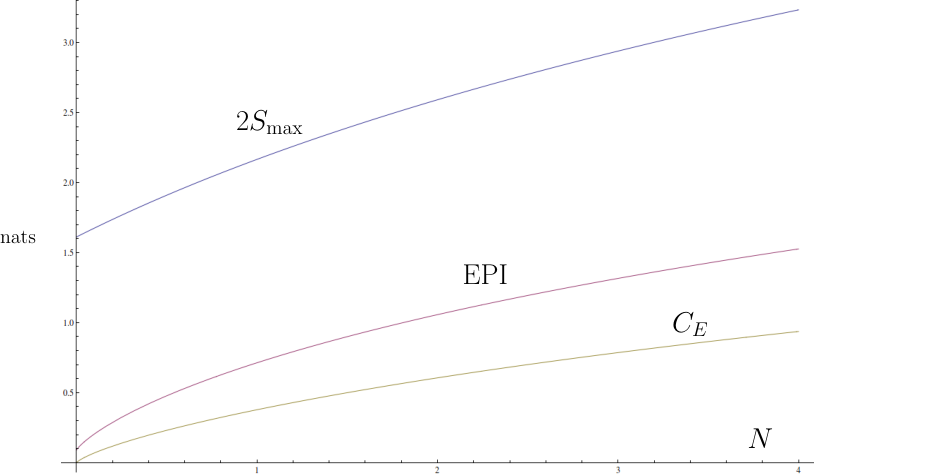
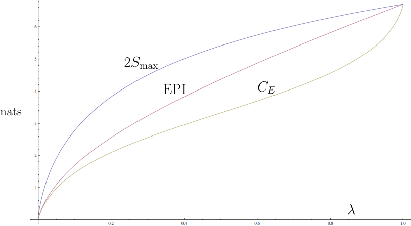
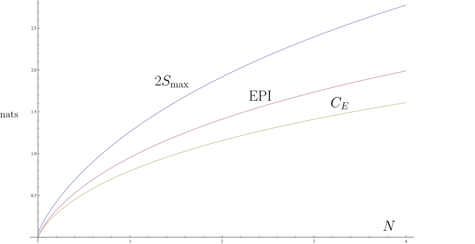
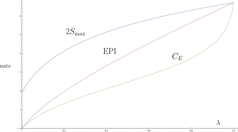
Figure 3 shows a comparison of this bound with the known capacity of the thermal noise channel.
Refer to caption
(a) 𝐍E=1/2{\bf N}_{E}=1/2, 𝐍=10{\bf N}=10 and λ∈[0,1]\lambda\in[0,1]
Refer to caption
(b) 𝐍E=1/2{\bf N}_{E}=1/2, λ=1/4\lambda=1/4 and 𝐍∈[0,4]{\bf N}\in[0,4]
Refer to caption
(c) 𝐍E=0.005{\bf N}_{E}=0.005, 𝐍=10{\bf N}=10 and λ∈[0,1]\lambda\in[0,1]
Refer to caption
(d) 𝐍E=0.005{\bf N}_{E}=0.005, λ=1/4\lambda=1/4 and 𝐍∈[0,4]{\bf N}\in[0,4]
Figure 3: Here we compare the upper bound of Corollary 3.1 with the known capacity of the thermal noise channel (with environment photon number 𝐍E{\bf N}_{E}). The latter is given by [18] the expression CE​(ℰλ,σE,𝐍)=g⁡(𝐍)+g⁡(𝐍max)−g⁡((D+𝐍max−𝐍−1)/2)−g⁡((D−𝐍max+𝐍−1)/2)C_{E}(\mathcal{E}_{\lambda,\sigma_{E}},{\bf N})=g({\bf N})+g({\bf N}_{\max})-g((D+{\bf N}_{\max}-{\bf N}-1)/2)-g((D-{\bf N}_{\max}+{\bf N}-1)/2), where D=(𝐍+𝐍max+1)2−4​λ​𝐍​(𝐍+1)D=\sqrt{({\bf N}+{\bf N}_{\max}+1)^{2}-4\lambda{\bf N}({\bf N}+1)}. We are interested in the case where σE\sigma_{E} is close to the vacuum state corresponding to a pure loss channel. We plot the capacity CEC_{E}, the EPI upper bound (8) and the maximum entropy upper bound (7). While in this case, the exact value of the capacity is known, these figures illustrate how the entropy power inequality improves over the trivial bound. Its insensitivity to the exact form of the environment’s state may be useful in certain applications. In contrast, the expression for CEC_{E} depends on the fact that σE\sigma_{E} is a thermal Gaussian state, that is, the gauge-invariance of ℰλ,σE\mathcal{E}_{\lambda,\sigma_{E}}.

Note that if the state σE\sigma_{E} is Gaussian, then the channel ℰλ,σE\mathcal{E}_{\lambda,\sigma_{E}} is a Gaussian operation. Various capacities of such channels have been studied in detail [18] (see [10] for a recent review). In particular, the entanglement-assisted capacity CE​(ℰλ,σE,𝐍)C_{E}(\mathcal{E}_{\lambda,\sigma_{E}},{\bf N}) is the result of a convex optimization problem: it is obtained by maximizing the mutual information over the (convex) set of covariance matrices MM associated with Gaussian states ρ\rho satisfying the photon number constraint22 2 This follows from the fact that the maximum mutual information in (6) is achieved on a Gaussian state ρ\rho and the concavity of I⁡(ℰ,ρ)I(\mathcal{E},\rho) in ρ\rho, see [18].. In principle, this can be addressed using efficient numerical algorithms. Furthermore, in special cases, it is possible to give an explicit expression for CE​(ℰλ,σE,𝐍)C_{E}(\mathcal{E}_{\lambda,\sigma_{E}},{\bf N}): Holevo and Werner [18] computed the entanglement-assisted capacity of the attenuation/amplification channel with classical noise (the most general one-mode channel not involving squeezing). Similarly, the entanglement-assisted capacity of the broadband lossy channel was discussed in detail in [11]. The crucial feature enabling these calculations is gauge-invariance of ℰλ,σE\mathcal{E}_{\lambda,\sigma_{E}}. Because the entanglement-assisted capacity is additive, this is equivalent to the state σE\sigma_{E} being thermal with respect to the mode operators defining the beam-splitter. In contrast, Corollary 3.1 gives a bound which is applicable to all Gaussian additive channels without further restrictions.

Recall that the entropy power inequality [21] provides an additive upper bound on the classical capacity of thermal noise channels. Because the entanglement-assisted capacity is additive, the conditional entropy power inequality plays a somewhat different role in Corollary 3.1: it substitutes an optimization problem by a bound depending on simple universal parameters (i.e., the entropy and the mean photon number of the environment). One may hope that the conditional entropy power inequality may also be used to address additivity problems in the context of entanglement-assisted communication. A natural candidate problem here is the rate region of the quantum multiple access channel (MAC) characterized by Hsieh, Devetak and Winter [19], where a single-letter formula is not known. The use of conditional entropy power inequalities is especially suggestive in the case of the additive bosonic MAC (see e.g., [35]), where Alice and Bob are connected to a receiver Charlie via two arms of a beamsplitter. As shown by Cezkaj et al. [7] (see also [8]), this scenario exhibits uniquely quantum activation effects: providing entanglement-assistance to Bob can boost Alice’s maximal rate of communication. This is in contrast to analogous classical settings, where providing additional resources to Bob cannot change her maximal rate (the latter is determined by her signal power). While the conditional entropy power inequality can be used to bound the strength of this activation effect, a direct application does unfortunately not appear to yield fundamental new insights into the additivity problem for the bosonic MAC.

Outline

In Section 4, we recall basic definitions. In Section 5, we perturbatively compute the first-order corrections to the symplectic eigenvalues of symmetric matrices relevant in our context. In Section 6, we apply these perturbative results to obtain the asymptotic scaling of the conditional entropy, as well as its infinitesimal rate of increase when part of a Gaussian state undergoes diffusion. In Section 7, we connect this to Fisher information by establishing a de Bruijin-type identity for conditional entropies. In Section 8, we complete the proof of the entropy power inequality for conditional entropies.

4 Basic definitions

Consider NN bosonic modes described by mode operators R→=(Q1,P1,…,QN,PN)\vec{R}=(Q_{1},P_{1},\ldots,Q_{N},P_{N}) satisfying the canonical commutation relations

[Rk,Rℓ]=i​Jk,ℓ where JN=(01−10)⊕N.\displaystyle[R_{k},R_{\ell}]=iJ_{k,\ell}\qquad\textrm{ where }\qquad J_{N}=\left(\begin{matrix}0&1\\ -1&0\end{matrix}\right)^{\oplus N}\ .

A Gaussian quantum state ρ=ρM,d→\rho=\rho_{M,\vec{d}} on this system is completely specified by its first and second moments, i.e., the displacement vector d→=(d1,…,d2​N)∈ℝ2​N\vec{d}=(d_{1},\ldots,d_{2N})\in\mathbb{R}^{2N} and its (symmetric) covariance matrix MM, defined by

dk=tr(ρ​Rk) and Mj,k=tr(ρ⁡{Rj−dj,Rk−dk}).\displaystyle d_{k}=\mathop{\mathrm{tr}}\nolimits(\rho R_{k})\qquad\textrm{ and }\qquad M_{j,k}=\mathop{\mathrm{tr}}\nolimits(\rho\{R_{j}-d_{j},R_{k}-d_{k}\})\ .

Here {A,B}=A​B+B​A\{A,B\}=AB+BA. We call ρM,0\rho_{M,0} a centered Gaussian state and often write ρM\rho_{M} for it.

A Gaussian operation maps Gaussian states to Gaussian states and is determined by its action on (M,d)(M,d). An example is a displacement (or Weyl) operator W⁡(ξ→)W(\vec{\xi}), ξ→∈ℝ2​N\vec{\xi}\in\mathbb{R}^{2N}: this is a unitary operation satisfying

W⁡(ξ→)​ρM,d→​W​(ξ→)†\displaystyle W(\vec{\xi})\rho_{M,\vec{d}}W(\vec{\xi})^{\dagger} =ρM,d→+ξ→,\displaystyle=\rho_{M,\vec{d}+\vec{\xi}}\ , (9)

for all Gaussian states ρM,d\rho_{M,d}. It will sometimes be convenient to write the conjugation map as 𝒲ξ→​(ρ):=W⁡(ξ→)​ρ​W​(ξ→)†\mathcal{W}_{\vec{\xi}}(\rho):=W(\vec{\xi})\rho W(\vec{\xi})^{\dagger} . Statement (9) is equivalent to the Heisenberg action on the mode operators

W​(ξ)†​Rk​W​(ξ)=Rk+ξk for all ​k=1,…,2​N.\displaystyle W(\xi)^{\dagger}R_{k}W(\xi)=R_{k}+\xi_{k}\qquad\textrm{ for all }k=1,\ldots,2N\ . (10)

A matrix SS satisyfing S​JN​ST=JNSJ_{N}S^{T}=J_{N} is called symplectic. A symplectic matrix SS uniquely defines a Gaussian unitary USU_{S} by the action on mode operators

US†​Rj​US\displaystyle U_{S}^{\dagger}R_{j}U_{S} =∑k=12​NSj,kRk=:Rj′ for all j=1,…,2N.\displaystyle=\sum_{k=1}^{2N}S_{j,k}R_{k}=:R_{j}^{\prime}\qquad\textrm{ for all }j=1,\ldots,2N\ . (11)

Because SS is symplectic, the transformed operators R→′=(R1′,…,R2​N′)=(Q1′,P1′,…,QN′,PN′)\vec{R}^{\prime}=(R_{1}^{\prime},\ldots,R_{2N}^{\prime})=(Q_{1}^{\prime},P_{1}^{\prime},\ldots,Q_{N}^{\prime},P_{N}^{\prime}) again satisfy canonical commutation relations. It is convenient to define the (transformed) creation and annihilation operators

ak†=12​(Qk′+i​Pk′) and ak=12​(Qk′−i​Pk′).\displaystyle a_{k}^{\dagger}=\frac{1}{\sqrt{2}}(Q^{\prime}_{k}+iP^{\prime}_{k})\qquad\textrm{ and }\qquad a_{k}=\frac{1}{\sqrt{2}}(Q_{k}^{\prime}-iP_{k}^{\prime})\ .

The associated number operators

n^k=ak†ak=12((Qk′)2+(Pk′)2)−12I,k=1,…,N\displaystyle\hat{n}_{k}=a_{k}^{\dagger}a_{k}=\frac{1}{2}((Q^{\prime}_{k})^{2}+(P^{\prime}_{k})^{2})-\frac{1}{2}I,\qquad k=1,\ldots,N\ (12)

are mutually commuting, and there is a simultaneous orthonormal eigenbasis of the form |n⟩=|n1,…,nk⟩|n\rangle=|n_{1},\ldots,n_{k}\rangle with n^k​|n⟩=nk​|n⟩\hat{n}_{k}|n\rangle=n_{k}|n\rangle.

Eq. (11) translates into the action

US​ρM,d​US†\displaystyle U_{S}\rho_{M,d}U_{S}^{\dagger} =ρS​M​ST,S​d,\displaystyle=\rho_{SMS^{T},Sd}\ , (13)

on the covariance matrix and the displacement vector. In particular, displacement operators and unitaries of the form USU_{S} can be used to diagonalize any Gaussian state (with (9) and (13)). More precisely, Williamson’s theorem [33] states that a symmetric positive definite matrix MM can be diagonalized by a symplectic matrix SS, i.e.,

S​M​ST=diag​(λ1,λ1,λ2,λ2,…,λN,λN)=:DN​(λ→).\displaystyle SMS^{T}=\mbox{diag}(\lambda_{1},\lambda_{1},\lambda_{2},\lambda_{2},\ldots,\lambda_{N},\lambda_{N})=:D_{N}(\vec{\lambda})\ . (14)

We call λ→=(λ1,…,λN)\vec{\lambda}=(\lambda_{1},\ldots,\lambda_{N}) the symplectic eigenvalues of MM. Observe that this list may include multiplicities (i.e., λi=λj\lambda_{i}=\lambda_{j} for i≠ji\neq j). We will occasionally denote the set of distinct symplectic eigenvalues as 𝖲𝗌𝗉𝖾𝖼⁡(M)\mathsf{Sspec}(M). The quantity Δ⁡(M)=minλ,λ~∈𝖲𝗌𝗉𝖾𝖼⁡(M),λ≠λ~⁡|λ−λ~|\Delta(M)=\min_{\lambda,\tilde{\lambda}\in\mathsf{Sspec}(M),\lambda\neq\tilde{\lambda}}|\lambda-\tilde{\lambda}| will be referred to as the symplectic gap of MM.

With (13), identity (14) implies that a centered Gaussian state ρM\rho_{M} with covariance matrix MM can be brought into product form as

US​ρM​US†=⨂j=1ne−βj​n^jtre−βj​n^j,\displaystyle U_{S}\rho_{M}U_{S}^{\dagger}=\bigotimes_{j=1}^{n}\frac{e^{-\beta_{j}\hat{n}_{j}}}{\mathop{\mathrm{tr}}\nolimits e^{-\beta_{j}\hat{n}_{j}}}\ , (15)

where the inverse temperatures βj=β⁡(λj)\beta_{j}=\beta(\lambda_{j}) are given in terms of the symplectic eigenvalues by

β⁡(λ)=log⁡λ+1λ−1.\displaystyle\beta(\lambda)=\log\frac{\lambda+1}{\lambda-1}\ . (16)

Note that β⁡(λ)\beta(\lambda) is monotonically decreasing with increasing λ\lambda, β⁡(λ)<2\beta(\lambda)<2 for λ>2\lambda>2, and limλ→∞β⁡(λ)=0\lim_{\lambda\rightarrow\infty}\beta(\lambda)=0. If λj=1\lambda_{j}=1, then the factor e−βj​n^jtre−βj​n^j\frac{e^{-\beta_{j}\hat{n}_{j}}}{\mathop{\mathrm{tr}}\nolimits e^{-\beta_{j}\hat{n}_{j}}} in (15) needs to be replaced by the pure ‘vacuum’ state |0⟩​⟨0|Qj′​Pj′|0\rangle\langle 0|_{Q_{j}^{\prime}P_{j}^{\prime}} associated the the mode operators Qj′Q^{\prime}_{j}, Pj′P^{\prime}_{j}. Eq. (15) shows that the number states {|n⟩}n∈ℕ0N\{|n\rangle\}_{n\in\mathbb{N}_{0}^{N}} corresponding to the transformed mode operators R→′\vec{R}^{\prime} are an eigenbasis of US​ρM​US†U_{S}\rho_{M}U_{S}^{\dagger}.

The entropy S(ρ)=−tr(ρlogρ)S(\rho)=-\mathop{\mathrm{tr}}\nolimits(\rho\log\rho) of an NN-mode Gaussian state ρ=ρM,d\rho=\rho_{M,d} only depends on the symplectic eigenvalues λ→=(λ1,…,λN)\vec{\lambda}=(\lambda_{1},\ldots,\lambda_{N}) of the covariance matrix. To express it, it is useful to define the mean photon number 𝐍⁡(λk){\bf N}(\lambda_{k}) in the eigenmode kk by the function

𝐍⁡(λ)=(λ−1)/2\displaystyle{\bf N}(\lambda)=(\lambda-1)/2 (17)

of a symplectic eigenvalue λ\lambda. Then the entropy is given by

S⁡(ρ)\displaystyle S(\rho) =∑j=1Ng(𝐍(λj)) with g(𝐍):=(𝐍+1)log(𝐍+1)−𝐍log𝐍.\displaystyle=\sum_{j=1}^{N}g({\bf N}(\lambda_{j}))\qquad\textrm{ with }\qquad g({\bf N}):=({\bf N}+1)\log({\bf N}+1)-{\bf N}\log{\bf N}\ . (18)

Let us give a simple bound on the dependence of the entropy on the symplectic eigenvalues.

Lemma 4.1.

Suppose ρ\rho and σ\sigma are NN-mode Gaussian states with (arbitrarily ordered) symplectic eigenvalues ν→=(ν1,…,νN)\vec{\nu}=(\nu_{1},\ldots,\nu_{N}) and λ→=(λ1,…,λN)\vec{\lambda}=(\lambda_{1},\ldots,\lambda_{N}), respectively, and assume that λj≠1\lambda_{j}\neq 1 for all j=1,…,Nj=1,\ldots,N. Let ‖ν→−λ→‖∞=max1≤j≤N⁡|νj−λj|\|\vec{\nu}-\vec{\lambda}\|_{\infty}=\max_{1\leq j\leq N}|\nu_{j}-\lambda_{j}| and λ∗=min1≤j≤N⁡λj\lambda_{*}=\min_{1\leq j\leq N}\lambda_{j}. Then

|S⁡(ρ)−S⁡(σ)|≤N2​(‖ν→−λ→‖∞​β​(λ∗)+‖ν→−λ→‖∞2λ∗2−1).\displaystyle|S(\rho)-S(\sigma)|\leq\frac{N}{2}\left(\|\vec{\nu}-\vec{\lambda}\|_{\infty}\beta(\lambda_{*})+\frac{\|\vec{\nu}-\vec{\lambda}\|_{\infty}^{2}}{\lambda_{*}^{2}-1}\right)\ .

The requirement that σ\sigma has no symplectic eigenvalue equal to 11 (or equivalently λ∗>1\lambda_{*}>1) implies that none of the eigenmodes factors out in a pure product state, and we can usually assume this without loss of generality in our considerations below.

Proof.

We have g′​(𝐍)=log⁡((𝐍+1)/𝐍)g^{\prime}({\bf N})=\log(({\bf N}+1)/{\bf N}), and combining this with (17), we obtain the inverse temperature according to

g′​(𝐍⁡(λ))=β⁡(λ).\displaystyle g^{\prime}({\bf N}(\lambda))=\beta(\lambda)\ . (19)

Furthermore, we have

β′​(λ)=−2λ2−1.\displaystyle\beta^{\prime}(\lambda)=-\frac{2}{\lambda^{2}-1}\ . (20)

Let us define the function G⁡(λ):=g⁡(𝐍⁡(λ))G(\lambda):=g({\bf N}(\lambda)). Because 𝐍′​(λ)=λ/2{\bf N}^{\prime}(\lambda)=\lambda/2, Eqs. (19) and (20) imply

G′​(λ)=β⁡(λ)/2 and G′′​(λ)=−1λ2−1.\displaystyle G^{\prime}(\lambda)=\beta(\lambda)/2\qquad\textrm{ and }\qquad G^{\prime\prime}(\lambda)=-\frac{1}{\lambda^{2}-1}\ .

Hence the Taylor series expansion gives

|G⁡(λ+ϵ)−G⁡(λ)|≤ϵ​β​(λ)/2+ϵ22​|λ2−1|.\displaystyle|G(\lambda+\epsilon)-G(\lambda)|\leq\epsilon\beta(\lambda)/2+\frac{\epsilon^{2}}{2|\lambda^{2}-1|}\ .

Since β\beta is monotonically decreasing, we get

maxj|G⁡(νj)−G⁡(λj)|≤12​maxk​|νk−λk|​β​(minj⁡λj)+maxk⁡|νk−λk|22​minj​|λj2−1|\displaystyle\max_{j}|G(\nu_{j})-G(\lambda_{j})|\leq\frac{1}{2}\max_{k}|\nu_{k}-\lambda_{k}|\beta(\min_{j}\lambda_{j})+\frac{\max_{k}|\nu_{k}-\lambda_{k}|^{2}}{2\min_{j}|\lambda_{j}^{2}-1|}\

The claim follows from this because S⁡(ρ)=∑j=1NG⁡(νj)S(\rho)=\sum_{j=1}^{N}G(\nu_{j}) and S⁡(σ)=∑j=1NG⁡(λj)S(\sigma)=\sum_{j=1}^{N}G(\lambda_{j}) . ∎

5 Perturbation theory for symplectic eigenvalues

We begin with a straightforward application of degenerate perturbation theory which is illustrative of the method. We will need slightly more involved statements for bipartite systems below (Lemma 5.2). Note that a similar perturbative analysis was used in a different context in [26, Appendix B].

Lemma 5.1 (Perturbation of symplectic spectrum to 00th order).

Let MM be a covariance matrix of NN modes and consider the symplectic eigenvalues λ→​(ϵ)=(λ1​(ϵ),…,λN​(ϵ))\vec{\lambda}(\epsilon)=(\lambda_{1}(\epsilon),\ldots,\lambda_{N}(\epsilon)) of

M∞​(ϵ)\displaystyle M^{\infty}(\epsilon) =I+ϵ​M,\displaystyle=I+\epsilon M\ ,

where we assume that ‖M‖=O⁡(1)\|M\|=O(1) and ϵ≪1\epsilon\ll 1. Then

λj​(ϵ)=1+O⁡(ϵ) for all ​j=1,…,N.\displaystyle\lambda_{j}(\epsilon)=1+O(\epsilon)\qquad\textrm{ for all }j=1,\ldots,N\ .
Proof.

The symplectic eigenvalues λ→​(ϵ)\vec{\lambda}(\epsilon) can be obtained from the spectrum 𝗌𝗉𝖾𝖼⁡(i​JN​M∞​(ϵ))\mathsf{spec}(iJ_{N}M^{\infty}(\epsilon)) of i​JN​M∞​(ϵ)iJ_{N}M^{\infty}(\epsilon) since this operator has eigenvalues (λ1​(ϵ),−λ1​(ϵ),…,λN​(ϵ),−λN​(ϵ))(\lambda_{1}(\epsilon),-\lambda_{1}(\epsilon),\ldots,\lambda_{N}(\epsilon),-\lambda_{N}(\epsilon)). Let us write

i​JN​M∞​(ϵ)\displaystyle iJ_{N}M^{\infty}(\epsilon) =H+V where H=iJN and V=iϵJNM.\displaystyle=H+V\qquad\textrm{ where }\qquad H=iJ_{N}\qquad\textrm{ and }\qquad V=i\epsilon J_{N}M\ .

Observe that the eigenvalues of HH are {1,−1}\{1,-1\} and ‖V‖=O⁡(ϵ)\|V\|=O(\epsilon). This means that we can apply standard degenerate perturbation theory: the spectrum 𝗌𝗉𝖾𝖼⁡(H+V)\mathsf{spec}(H+V) is given by

{μ+𝗌𝗉𝖾𝖼⁡(V|ℋμ)|μ∈𝗌𝗉𝖾𝖼⁡(H)}+O⁡(ϵ2)\displaystyle\{\mu+\mathsf{spec}(V|_{\mathcal{H}_{\mu}})\ \big|\ \mu\in\mathsf{spec}(H)\}+O(\epsilon^{2}) (21)

to first order in ϵ\epsilon, where V|ℋμV|_{\mathcal{H}_{\mu}} denotes the restriction of VV to the degenerate eigenspace ℋμ\mathcal{H}_{\mu} of HH to eigenvalue μ\mu. An immediate consequence is that (by assumption on ‖M‖\|M\|), the symplectic eigenvalues of M∞​(ϵ)M^{\infty}(\epsilon) are of the form λj​(ϵ)=1+O⁡(ϵ)\lambda_{j}(\epsilon)=1+O(\epsilon) for all j=1,…,Nj=1,\ldots,N. ∎

To obtain the correct constant (i.e., the first-order correction in (21)), it is necessary to compute the restriction V|ℋμV|_{\mathcal{H}_{\mu}} to the eigenspace with eigenvalue μ\mu. For this purpose, it is convenient to use a basis of ℋμ\mathcal{H}_{\mu}. For example, for the case of Lemma 5.1, we can define the vectors

|v+⟩=12​(i,1)=12​(i⁡|1⟩+|2⟩) and |v−⟩=12​(1,i)=12​(|1⟩+i⁡|2⟩)\displaystyle|v^{+}\rangle=\frac{1}{\sqrt{2}}(i,1)=\frac{1}{\sqrt{2}}(i|1\rangle+|2\rangle)\qquad\textrm{ and }\qquad|v^{-}\rangle=\frac{1}{\sqrt{2}}(1,i)=\frac{1}{\sqrt{2}}(|1\rangle+i|2\rangle)\

in ℝ2\mathbb{R}^{2} (Here and below, we will often use |j⟩|j\rangle to denote standard orthonormal basis vectors in ℝ2​N\mathbb{R}^{2N}.) Importantly, these vectors satisfy

i​J1​|v±⟩=±|v±⟩,\displaystyle iJ_{1}|v^{\pm}\rangle=\pm|v^{\pm}\rangle\ , (22)

and

⟨v±|i​J1​D1​(α)|v±⟩=±α⟨v∓|i​J1​D1​(α)|v±⟩=0 for all ​α∈ℝ.\displaystyle\langle v^{\pm}|iJ_{1}D_{1}(\alpha)|v^{\pm}\rangle=\pm\alpha\qquad\langle v^{\mp}|iJ_{1}D_{1}(\alpha)|v^{\pm}\rangle=0\qquad\textrm{ for all }\alpha\in\mathbb{R}\ . (23)

Writing (0,0)⊕k=(0,0)⊕⋯⊕(0,0)(0,0)^{\oplus k}=(0,0)\oplus\cdots\oplus(0,0) (kk summands), we can define

|vj,N±⟩=(0,0)(j−1)⊕|v±⟩⊕(0,0)⊕(N−j−1).\displaystyle|v_{j,N}^{\pm}\rangle=(0,0)^{(j-1)}\oplus|v^{\pm}\rangle\oplus(0,0)^{\oplus(N-j-1)}\ .

where |v±⟩|v^{\pm}\rangle is at mode jj (of NN modes).

Because of (22), the eigenspace ℋ1\mathcal{H}_{1} of HH to eigenvalue 11 has orthonormal basis {|vj,N+⟩}j=1,…,N\{|v_{j,N}^{+}\rangle\}_{j=1,\ldots,N}. Similarly, the eigenspace ℋ−1\mathcal{H}_{-1} has orthonormal basis {|vj,N−⟩}j=1,…,N\{|v_{j,N}^{-}\rangle\}_{j=1,\ldots,N}. The restriction of VV to ℋ1\mathcal{H}_{1} is given by the matrix (⟨vj+|V|vk+⟩)j,k=1,…,N(\langle v_{j}^{+}|V|v_{k}^{+}\rangle)_{j,k=1,\ldots,N}, and diagonalizing this matrix gives the first-order corrections to the eigenvalue 11 (the degeneracy is lifted). We will omit a more detailed discussion here as we will need a more general version (including a reference system BB). However, the proof of the following Lemma proceeds in this fashion; the key here is to apply perturbation theory to a suitably transformed matrix.

Lemma 5.2 (Perturbation of symplectic spectrum to 11st order).

Let

MA​B\displaystyle M_{AB} =(MALA​BLA​BTMB)\displaystyle=\left(\begin{matrix}M_{A}&L_{AB}\\ L_{AB}^{T}&M_{B}\end{matrix}\right)

be the covariance matrix of a state on m+nm+n modes with respect to the ordering

R→=(Q1A,P1A,…,QmA,PmA,Q1B,P1B,…,QnB,PnB)\displaystyle\vec{R}=(Q_{1}^{A},P_{1}^{A},\ldots,Q_{m}^{A},P_{m}^{A},Q_{1}^{B},P_{1}^{B},\ldots,Q_{n}^{B},P_{n}^{B})

of modes.

  1. (i)

    Assume that ‖MA​B‖=O⁡(1)\|M_{AB}\|=O(1) and ϵ≪1\epsilon\ll 1. Then the symplectic eigenvalues λ→​(ϵ)=(λ1​(ϵ),…,λm+n​(ϵ))\vec{\lambda}(\epsilon)=(\lambda_{1}(\epsilon),\ldots,\lambda_{m+n}(\epsilon)) of the covariance matrix

    MA​B∞​(ϵ)\displaystyle M^{\infty}_{AB}(\epsilon) =(IA000)+ϵ​MA​B=:IA⊕0B+ϵ​MA​B\displaystyle=\left(\begin{matrix}I_{A}&0\\ 0&0\end{matrix}\right)+\epsilon M_{AB}=:I_{A}\oplus 0_{B}+\epsilon M_{AB} (24)

    are of the form

    λj​(ϵ)=ηj​(ϵ)+O⁡(ϵ2)​ for ​j=1,…,m and λm+j​(ϵ)=ϵ​νj+O⁡(ϵ2)​ for ​j=1,…,n\displaystyle\lambda_{j}(\epsilon)=\eta_{j}(\epsilon)+O(\epsilon^{2})\ \textrm{ for }j=1,\ldots,m\quad\textrm{ and }\quad\lambda_{m+j}(\epsilon)=\epsilon\nu_{j}+O(\epsilon^{2})\ \textrm{ for }j=1,\ldots,n\

    where η→​(ϵ)=(η1​(ϵ),…,ηm​(ϵ))\vec{\eta}(\epsilon)=(\eta_{1}(\epsilon),\ldots,\eta_{m}(\epsilon)) are the eigenvalues of IA+ϵ​MAI_{A}+\epsilon M_{A} and ν→=(ν1,…,νn)\vec{\nu}=(\nu_{1},\ldots,\nu_{n}) are the eigenvalues of MBM_{B}.

  2. (ii)

    Let λ→=(λ1,…,λm+n)\vec{\lambda}=(\lambda_{1},\ldots,\lambda_{m+n}) be the symplectic eigenvalues of MA​BM_{AB} and let SA​BS_{AB} be the symplectic matrix diagonalizing MA​BM_{AB}, i.e.,

    SA​B​MA​B​SA​BT\displaystyle S_{AB}M_{AB}S_{AB}^{T} =Dm+n​(λ→).\displaystyle=D_{m+n}(\vec{\lambda})\ .

    Suppose ϵ≪Δ⁡(MA​B)\epsilon\ll\Delta(M_{AB}). Let λ→​(ϵ)=(λ1​(ϵ),…,λm+n​(ϵ))\vec{\lambda}(\epsilon)=(\lambda_{1}(\epsilon),\ldots,\lambda_{m+n}(\epsilon)) be the symplectic eigenvalues of

    MA​B0​(ϵ)\displaystyle M^{0}_{AB}(\epsilon) =MA​B+ϵ​IA⊕0B.\displaystyle=M_{AB}+\epsilon I_{A}\oplus 0_{B}\ . (25)

    Then degeneracies are split according to

    |{ℓ|λℓ=λ}|=|{ℓ|λℓ​(ϵ)∈[λ−Δ/2,λ+Δ/2]}\displaystyle|\{\ell\ |\ \lambda_{\ell}=\lambda\}|=|\{\ell\ |\ \lambda_{\ell}(\epsilon)\in[\lambda-\Delta/2,\lambda+\Delta/2]\} (26)

    where ℓ\ell ranges over ℓ∈{1,…,m+n}\ell\in\{1,\ldots,m+n\}. Furthermore

    ∑ℓ:λℓ​(ϵ)∈[λ−Δ/2,λ+Δ/2]λℓ(ϵ)\displaystyle\sum_{\ell:\lambda_{\ell}(\epsilon)\in[\lambda-\Delta/2,\lambda+\Delta/2]}\lambda_{\ell}(\epsilon) =∑ℓ:λℓ=λ(λ+ϵ2tr[SA​B(IA⊕0B)SA​BT](ℓ))+O(ϵ2)\displaystyle=\sum_{\ell:\lambda_{\ell}=\lambda}\left(\lambda+\frac{\epsilon}{2}\mathop{\mathrm{tr}}\nolimits[S_{AB}(I_{A}\oplus 0_{B})S_{AB}^{T}]^{(\ell)}\right)+O(\epsilon^{2})\

    for each λ∈𝖲𝗌𝗉𝖾𝖼⁡(MA​B)\lambda\in\mathsf{Sspec}(M_{AB}). Here [Z](ℓ)[Z]^{(\ell)} denotes the submatrix corresponding to the ℓ\ell-th mode, i.e., the 2×22\times 2-matrix with entries ([Z](ℓ))i,j=Z2​ℓ−1+i,2​ℓ−1+j([Z]^{(\ell)})_{i,j}=Z_{2\ell-1+i,2\ell-1+j}, i,j∈{0,1}i,j\in\{0,1\}.

Proof of Lemma 5.2 (i)

Our goal is to compute the symplectic eigenvalues λ1​(ϵ),…,λm+n​(ϵ)\lambda_{1}(\epsilon),\ldots,\lambda_{m+n}(\epsilon) of the covariance matrix

MA​B∞​(ϵ)\displaystyle M^{\infty}_{AB}(\epsilon) =IA⊕0B+ϵ​MA​B,\displaystyle=I_{A}\oplus 0_{B}+\epsilon M_{AB}\ ,

to first order in ϵ\epsilon. Let ν→=(ν1,…,νm)\vec{\nu}=(\nu_{1},\ldots,\nu_{m}) be the symplectic eigenvalues of MBM_{B}, and let SBS_{B} be the symplectic matrix diagonalizing MBM_{B}, i.e.,

SB​MB​SBT\displaystyle S_{B}M_{B}S_{B}^{T} =Dn​(ν→),\displaystyle=D_{n}(\vec{\nu})\ ,

where Dn​(ν→)=diag​(ν1,ν1)⊕⋯⊕diag​(νn,νn)D_{n}(\vec{\nu})=\mbox{diag}(\nu_{1},\nu_{1})\oplus\cdots\oplus\mbox{diag}(\nu_{n},\nu_{n}). Similarly, let α→​(ϵ)=(α1​(ϵ),…,αm​(ϵ))\vec{\alpha}(\epsilon)=(\alpha_{1}(\epsilon),\ldots,\alpha_{m}(\epsilon)) be such that the symplectic eigenvalues of IA+ϵ​MAI_{A}+\epsilon M_{A} are equal to (1+α1​(ϵ),…,1+αm​(ϵ))(1+\alpha_{1}(\epsilon),\ldots,1+\alpha_{m}(\epsilon)). Observe that

|αj​(ϵ)|=O⁡(ϵ) for ​j=1,…,m.\displaystyle|\alpha_{j}(\epsilon)|=O(\epsilon)\qquad\textrm{ for }j=1,\ldots,m\ . (27)

Let SA​(ϵ)S_{A}(\epsilon) be the symplectic matrix diagonalizing IA+ϵ​MAI_{A}+\epsilon M_{A}, i.e.,

SA​(ϵ)​(IA+ϵ​MA)​SA​(ϵ)T\displaystyle S_{A}(\epsilon)(I_{A}+\epsilon M_{A})S_{A}(\epsilon)^{T} =IA+Dm​(α→​(ϵ)).\displaystyle=I_{A}+D_{m}(\vec{\alpha}(\epsilon))\ .

Finally, let SA​B​(ϵ)=SA​(ϵ)⊕SBS_{AB}(\epsilon)=S_{A}(\epsilon)\oplus S_{B}. The symplectic spectrum of MA​B∞​(ϵ)M^{\infty}_{AB}(\epsilon) is identical to that of

M^A​B∞​(ϵ):=SA​B​(ϵ)​MA​B∞​(ϵ)​SA​B​(ϵ)T=(IA+Dm​(α→​(ϵ))ϵ​SA​(ϵ)​LA​B​SBTϵ​SB​LA​BT​SA​(ϵ)Tϵ​Dn​(ν→)).\displaystyle\hat{M}^{\infty}_{AB}(\epsilon):=S_{AB}(\epsilon)M^{\infty}_{AB}(\epsilon)S_{AB}(\epsilon)^{T}=\left(\begin{matrix}I_{A}+D_{m}(\vec{\alpha}(\epsilon))&\epsilon S_{A}(\epsilon)L_{AB}S_{B}^{T}\\ \epsilon S_{B}L^{T}_{AB}S_{A}(\epsilon)^{T}&\epsilon D_{n}(\vec{\nu})\end{matrix}\right)\ .

In particular, the eigenvalues of the matrix i​Jm+n​M^A​B∞​(ϵ)iJ_{m+n}\hat{M}^{\infty}_{AB}(\epsilon) are given by

𝗌𝗉𝖾𝖼⁡(i​Jm+n​M^A​B∞​(ϵ))=(λ1​(ϵ),−λ1​(ϵ),…,λm+n​(ϵ),−λm+n​(ϵ)).\displaystyle\mathsf{spec}(iJ_{m+n}\hat{M}_{AB}^{\infty}(\epsilon))=(\lambda_{1}(\epsilon),-\lambda_{1}(\epsilon),\ldots,\lambda_{m+n}(\epsilon),-\lambda_{m+n}(\epsilon))\ . (28)

Since Jm+n=Jm⊕JnJ_{m+n}=J_{m}\oplus J_{n}, we obtain

i​J​M^A​B∞​(ϵ)=H+V where ​H=(i​Jm000)​ and ​V=(i​Jm​Dm​(α→​(ϵ))Jm​X​(ϵ)Jn​X​(ϵ)Ti​ϵ​Jn​Dn​(ν→)),\displaystyle iJ\hat{M}^{\infty}_{AB}(\epsilon)=H+V\qquad\textrm{ where }H=\left(\begin{matrix}iJ_{m}&0\\ 0&0\end{matrix}\right)\ \textrm{ and }\ V=\left(\begin{matrix}iJ_{m}D_{m}(\vec{\alpha}(\epsilon))&J_{m}X(\epsilon)\\ J_{n}X(\epsilon)^{T}&i\epsilon J_{n}D_{n}(\vec{\nu})\end{matrix}\right)\ ,

where we introduced the abbreviation X⁡(ϵ)=i​ϵ​SA​(ϵ)​LA​B​SBTX(\epsilon)=i\epsilon S_{A}(\epsilon)L_{AB}S_{B}^{T}. By the assumption ‖MA​B‖=O⁡(1)\|M_{AB}\|=O(1), we have ‖X⁡(ϵ)‖=O⁡(ϵ)\|X(\epsilon)\|=O(\epsilon) and ‖Dn​(ν→)‖=O⁡(1)\|D_{n}(\vec{\nu})\|=O(1). Similarly, we have ‖Dm​(α→​(ϵ))‖=O⁡(ϵ)\|D_{m}(\vec{\alpha}(\epsilon))\|=O(\epsilon) because of Eq. (27). We conclude that ‖V‖=O⁡(ϵ)\|V\|=O(\epsilon). On the other hand, the eigenvalues of HH are {0,1,−1}\{0,1,-1\}, hence we can apply first-order (degenerate) perturbation theory to compute the spectrum of i​J​M^A​B∞​(ϵ)iJ\hat{M}^{\infty}_{AB}(\epsilon).

We consider the eigenspaces separately.

  • •

    μ=0\mu=0: Consider the eigenspace ℋ0\mathcal{H}_{0} of HH to eigenvalue μ=0\mu=0. It is easy to check that the vectors {v1,B+,v1,B−,…,vn,B+,vn,B−}\{v^{+}_{1,B},v^{-}_{1,B},\ldots,v^{+}_{n,B},v^{-}_{n,B}\} defined by

    |vj,B±⟩:=0A⊕|vj,n±⟩\displaystyle|v_{j,B}^{\pm}\rangle:=0_{A}\oplus|v_{j,n}^{\pm}\rangle\

    are an orthonormal basis of ℋ0\mathcal{H}_{0}. (Here we write 0A0_{A} for the zero-vector (0,0)⊕m(0,0)^{\oplus m}.) Since

    V​|vk,Bτ⟩\displaystyle V|v_{k,B}^{\tau}\rangle =(Jm​X​|vk,nτ⟩)⊕(i​ϵ​Jn​Dn​(ν)​|vk,nτ⟩),\displaystyle=(J_{m}X|v_{k,n}^{\tau}\rangle)\oplus(i\epsilon J_{n}D_{n}(\nu)|v_{k,n}^{\tau}\rangle)\ ,

    we get the matrix elements

    ⟨vj,Bσ|V|vk,Bτ⟩\displaystyle\langle v_{j,B}^{\sigma}|V|v_{k,B}^{\tau}\rangle =⟨vj,nσ|i​ϵ​Jn​Dn​(ν→)|vk,nτ⟩=δj,k​δσ,τ​(σ⋅ϵ​νj)\displaystyle=\langle v_{j,n}^{\sigma}|i\epsilon J_{n}D_{n}(\vec{\nu})|v_{k,n}^{\tau}\rangle=\delta_{j,k}\delta_{\sigma,\tau}(\sigma\cdot\epsilon\nu_{j})\

    according to (23). In particular, the restriction V|ℋ0V|_{\mathcal{H}_{0}} is described by a diagonal matrix with diagonal elements of the form {±ϵ​νj}j=1n\{\pm\epsilon\nu_{j}\}_{j=1}^{n}. With (21), we have found mm symplectic eigenvalues of the form

    λm+j​(ϵ)=ϵ​νj+O⁡(ϵ2) for ​j=1,…,n.\displaystyle\lambda_{m+j}(\epsilon)=\epsilon\nu_{j}+O(\epsilon^{2})\qquad\textrm{ for }j=1,\ldots,n\ . (29)

    (Only the non-negative entries on the diagonal are symplectic eigenvalues according to (28).) Note that these are simply the eigenvalues of MBM_{B}, up to a factor of ϵ\epsilon.

  • •

    μ=1\mu=1: An orthonormal basis of ℋ1\mathcal{H}_{1} is given by the vectors {|vj,A+⟩}j=1m\{|v_{j,A}^{+}\rangle\}_{j=1}^{m} defined by

    |vj,A+⟩:=|vj,m±⟩⊕0B\displaystyle|v_{j,A}^{+}\rangle:=|v_{j,m}^{\pm}\rangle\oplus 0_{B}\

    where 0B0_{B} stands for (0,0)⊕n(0,0)^{\oplus n}. It is easy to check that

    ⟨vj,A+|V|vk,B+⟩=δj,k​αj​(ϵ),\displaystyle\langle v_{j,A}^{+}|V|v_{k,B}^{+}\rangle=\delta_{j,k}\alpha_{j}(\epsilon)\ ,

    i.e., the restriction of VV to ℋ1\mathcal{H}_{1} is diagonal when expressed in this basis. In conclusion, we found mm symplectic eigenvalues of the form

    λj​(ϵ)=1+αj​(ϵ)+O⁡(ϵ2) for ​j=1,…,m.\displaystyle\lambda_{j}(\epsilon)=1+\alpha_{j}(\epsilon)+O(\epsilon^{2})\qquad\textrm{ for }j=1,\ldots,m\ . (30)

    By definition of αj​(ϵ)\alpha_{j}(\epsilon), these are equal to the symplectic eigenvalues ηj​(ϵ)=1+αj​(ϵ)\eta_{j}(\epsilon)=1+\alpha_{j}(\epsilon) of IA+ϵ​MAI_{A}+\epsilon M_{A} in order O⁡(ϵ)O(\epsilon).

  • •

    μ=−1\mu=-1: Here we find an orthonormal basis with vectors |vj,A+⟩:=|vj,m+⟩⊕0B|v_{j,A}^{+}\rangle:=|v_{j,m}^{+}\rangle\oplus 0_{B}. The restriction of VV to ℋ−1\mathcal{H}_{-1} is diagonal with diagonal entries (−α1​(ϵ),…,−αm​(ϵ))(-\alpha_{1}(\epsilon),\ldots,-\alpha_{m}(\epsilon)). The corresponding eigenvalues are the negatives of (30), consistent with (28).

Proof of Lemma 5.2 (ii)

Let us briefly recall the definitions involved in the statement. We consider the covariance matrix

MA​B0​(ϵ)\displaystyle M^{0}_{AB}(\epsilon) =MA​B+ϵ⁡(IA000)=MA​B+ϵ​IA⊕0B,\displaystyle=M_{AB}+\epsilon\left(\begin{matrix}I_{A}&0\\ 0&0\end{matrix}\right)=M_{AB}+\epsilon I_{A}\oplus 0_{B}\ ,

where MA​BM_{AB} has symplectic eigenvalues λ→=(λ1,…,λm+n)\vec{\lambda}=(\lambda_{1},\ldots,\lambda_{m+n}) and is diagonalized by SA​BS_{AB}, i.e.,

SA​B​MA​B​SA​BT=Dm+n​(λ→).\displaystyle S_{AB}M_{AB}S_{AB}^{T}=D_{m+n}(\vec{\lambda})\ .

We assume that ϵ≪Δ\epsilon\ll\Delta, where Δ=Δ⁡(MA​B)\Delta=\Delta(M_{AB}) is the symplectic gap. Then MA​B0​(ϵ)M^{0}_{AB}(\epsilon) has the same symplectic eigenvalues as

M^A​B0​(ϵ)=Dm+n​(λ→)+ϵ​SA​B​(IA⊕0B)​SA​BT.\displaystyle\hat{M}^{0}_{AB}(\epsilon)=D_{m+n}(\vec{\lambda})+\epsilon S_{AB}(I_{A}\oplus 0_{B})S_{AB}^{T}\ .

In particular, it suffices to find the eigenvalues of

i​Jm+n​M^A​B0​(ϵ)=i​Jm+n​Dm+n​(λ→)+i​ϵ​Jm+n​SA​B​(IA⊕0B)​SA​BT=:H+V.\displaystyle iJ_{m+n}\hat{M}^{0}_{AB}(\epsilon)=iJ_{m+n}D_{m+n}(\vec{\lambda})+i\epsilon J_{m+n}S_{AB}(I_{A}\oplus 0_{B})S_{AB}^{T}=:H+V\ .

Because H:=i​Jm+n​Dm+n​(λ→)H:=iJ_{m+n}D_{m+n}(\vec{\lambda}) has gap Δ\Delta, ‖i​Jm+n​SA​B​(IA⊕0B)​SA​BT‖=O⁡(1)\|iJ_{m+n}S_{AB}(I_{A}\oplus 0_{B})S_{AB}^{T}\|=O(1) and our assumption ϵ≪Δ\epsilon\ll\Delta, we can apply (degenerate) perturbation theory to compute the spectrum of i​J​M^A​B0​(ϵ)iJ\hat{M}^{0}_{AB}(\epsilon).

The operator HH has eigenvectors (w1+,…,wm+n+)=(v1,A+,…,vm,A+,v1,B+,…,vn,B+)(w_{1}^{+},\ldots,w_{m+n}^{+})=(v_{1,A}^{+},\ldots,v_{m,A}^{+},v_{1,B}^{+},\ldots,v_{n,B}^{+}) with eigenvalues λ1,…,λm+n\lambda_{1},\ldots,\lambda_{m+n}. In particular, for λ∈𝖲𝗌𝗉𝖾𝖼⁡(MA​B)\lambda\in\mathsf{Sspec}(M_{AB}), the eigenspace ℋλ\mathcal{H}_{\lambda} of HH is

ℋλ\displaystyle\mathcal{H}_{\lambda} =span⁡{|wℓ+⟩| 1≤ℓ≤m+n​ with ​λℓ=λ}.\displaystyle=\mathrm{span}\{|w_{\ell}^{+}\rangle\ |\ 1\leq\ell\leq m+n\textrm{ with }\lambda_{\ell}=\lambda\}\ .

Suppose that restriction V|ℋλV|_{\mathcal{H}_{\lambda}} of V:=i​ϵ​Jm+n​SA​B​(IA⊕0B)​SA​BTV:=i\epsilon J_{m+n}S_{AB}(I_{A}\oplus 0_{B})S_{AB}^{T} to ℋλ\mathcal{H}_{\lambda} has eigenvalues θ1,…,θdimℋλ\theta_{1},\ldots,\theta_{\dim\mathcal{H}_{\lambda}}. According to (degenerate) first-order perturbation theory, the matrix i​Jm+n​M^A​B0​(ϵ)iJ_{m+n}\hat{M}^{0}_{AB}(\epsilon) has dimℋλ\dim\mathcal{H}_{\lambda} eigenvalues of the form

λ+θj+O⁡(ϵ2) for ​j=1,…,dimℋλ,\displaystyle\lambda+\theta_{j}+O(\epsilon^{2})\qquad\textrm{ for }j=1,\ldots,\dim\mathcal{H}_{\lambda}\ , (31)

where θj=O⁡(ϵ)\theta_{j}=O(\epsilon). Furthermore, the list (31) includes all eigenvalues λℓ​(ϵ)\lambda_{\ell}(\epsilon) of i​Jm+n​M^A​B0​(ϵ)iJ_{m+n}\hat{M}^{0}_{AB}(\epsilon) in the interval [λ−Δ/2,λ+Δ/2][\lambda-\Delta/2,\lambda+\Delta/2] and the number of such eigenvalues is equal to (26) by the assumption ϵ≪Δ\epsilon\ll\Delta. We conclude that

∑ℓ:λℓ​(ϵ)∈[λ−Δ/2,λ+Δ/2]λℓ(ϵ)\displaystyle\sum_{\ell:\lambda_{\ell}(\epsilon)\in[\lambda-\Delta/2,\lambda+\Delta/2]}\lambda_{\ell}(\epsilon) =(dimℋλ)⋅λ+∑j=1dimℋλθj+O⁡(ϵ2)\displaystyle=(\dim\mathcal{H}_{\lambda})\cdot\lambda+\sum_{j=1}^{\dim\mathcal{H}_{\lambda}}\theta_{j}+O(\epsilon^{2})
=(dimℋλ)⋅λ+tr(V|ℋλ)+O⁡(ϵ2)\displaystyle=(\dim\mathcal{H}_{\lambda})\cdot\lambda+\mathop{\mathrm{tr}}\nolimits(V|_{\mathcal{H}_{\lambda}})+O(\epsilon^{2}) (32)

Because the restriction V|ℋV|_{\mathcal{H}} can be expressed as

V|ℋλ\displaystyle V|_{\mathcal{H}_{\lambda}} =∑j,k:λj=λk=λ⟨wj+|V|wk+⟩⋅|wj+⟩⟨wk+|,\displaystyle=\sum_{j,k:\lambda_{j}=\lambda_{k}=\lambda}\langle w^{+}_{j}|V|w^{+}_{k}\rangle\cdot|w^{+}_{j}\rangle\langle w^{+}_{k}|\ ,

we obtain

tr(V|ℋλ)\displaystyle\mathop{\mathrm{tr}}\nolimits(V|_{\mathcal{H}_{\lambda}}) =iϵ∑ℓ:λℓ=λ⟨wℓ+|Jm+nSA​B(IA⊕0B)SA​BT|wℓ+⟩.\displaystyle=i\epsilon\sum_{\ell:\lambda_{\ell}=\lambda}\langle w_{\ell}^{+}|J_{m+n}S_{AB}(I_{A}\oplus 0_{B})S_{AB}^{T}|w_{\ell}^{+}\rangle\ . (33)

Combining (33) with dimℋλ=|{ℓ:λℓ=λ}|\dim\mathcal{H}_{\lambda}=|\{\ell:\lambda_{\ell}=\lambda\}| and Eq. (32) gives

∑ℓ:λℓ​(ϵ)∈[λ−Δ/2,λ+Δ/2]λℓ(ϵ)=∑ℓ:λℓ=λ(λ+iϵ⟨wℓ+|Jm+nSA​B(IA⊕0B)SA​BT|wℓ+⟩)+O(ϵ2).\displaystyle\sum_{\ell:\lambda_{\ell}(\epsilon)\in[\lambda-\Delta/2,\lambda+\Delta/2]}\lambda_{\ell}(\epsilon)=\sum_{\ell:\lambda_{\ell}=\lambda}\left(\lambda+i\epsilon\langle w_{\ell}^{+}|J_{m+n}S_{AB}(I_{A}\oplus 0_{B})S_{AB}^{T}|w_{\ell}^{+}\rangle\right)+O(\epsilon^{2})\ . (34)

Since |wℓ+⟩=12​(i⁡|2​ℓ−1⟩+|2​ℓ⟩)|w_{\ell}^{+}\rangle=\frac{1}{\sqrt{2}}(i|2\ell-1\rangle+|2\ell\rangle) and Jm+n=∑k=1m+n|2​k−1⟩​⟨2​k|−|2​k⟩​⟨2​k−1|J_{m+n}=\sum_{k=1}^{m+n}|2k-1\rangle\langle 2k|-|2k\rangle\langle 2k-1|, we have ⟨wℓ+|​Jm+n=12​(i⁡⟨2​ℓ|+⟨2​ℓ−1|)\langle w_{\ell}^{+}|J_{m+n}=\frac{1}{\sqrt{2}}(i\langle 2\ell|+\langle 2\ell-1|), and this takes the form

⟨wℓ+|Jm+n​SA​B​(IA⊕0B)​SA​BT|wℓ+⟩=12​(i​Z2​ℓ,2​ℓ−1−i​Z2​ℓ−1,2​ℓ+Z2​ℓ,2​ℓ+Z2​ℓ−1,2​ℓ−1)\displaystyle\langle w_{\ell}^{+}|J_{m+n}S_{AB}(I_{A}\oplus 0_{B})S_{AB}^{T}|w_{\ell}^{+}\rangle=\frac{1}{2}\left(iZ_{2\ell,2\ell-1}-iZ_{2\ell-1,2\ell}+Z_{2\ell,2\ell}+Z_{2\ell-1,2\ell-1}\right)\

where Z=SA​B​(IA⊕0B)​SA​BTZ=S_{AB}(I_{A}\oplus 0_{B})S_{AB}^{T}. Since ZT=ZZ^{T}=Z is symmetric, this is equal to

⟨wℓ+|Jm+n​SA​B​(IA⊕0B)​SA​BT|wℓ+⟩=12​tr[SA​B​(IA⊕0B)​SA​BT](ℓ),\displaystyle\langle w_{\ell}^{+}|J_{m+n}S_{AB}(I_{A}\oplus 0_{B})S_{AB}^{T}|w_{\ell}^{+}\rangle=\frac{1}{2}\mathop{\mathrm{tr}}\nolimits[S_{AB}(I_{A}\oplus 0_{B})S_{AB}^{T}]^{(\ell)}\ , (35)

and the claim follows by inserting (35) into (34).

6 Conditional entropy and diffusion

A central tool in the proof of the quantum entropy power inequality [20] is the one-parameter semigroup {et​ℒ}t≥0\{e^{t\mathcal{L}}\}_{t\geq 0} of completely positive trace-preserving maps generated by the ‘diffusion’ Liouvillean ℒ\mathcal{L} (see [20] for a definition of the latter). For all t≥0t\geq 0, the map et​ℒe^{t\mathcal{L}} is Gaussian and can therefore be defined in terms of its action on the covariance matrix MM and the displacement vector d→\vec{d}: A Gaussian state ρ\rho described by (M,d→)(M,\vec{d}) is transformed into a Gaussian state ρ​(t)=et​ℒ​(ρ)\rho(t)=e^{t\mathcal{L}}(\rho) with covariance matrix (M⁡(t)=M+t​I,d→)(M(t)=M+tI,\vec{d}), i.e., the transformation governing the evolution for time tt is

ρ↦et​ℒ​(ρ)(M,d→)↦et​ℒ(M+t​I,d→) for all covariance matrices ​M​ and displacement vectors ​d→.\displaystyle\begin{matrix}\rho&\mapsto&e^{t\mathcal{L}}(\rho)\\ (M,\vec{d})&\overset{e^{t\mathcal{L}}}{\mapsto}&(M+tI,\vec{d})\end{matrix}\qquad\textrm{ for all covariance matrices }M\textrm{ and displacement vectors }\vec{d}\ .

In this section, we revisit and extend statements of [20] about the behavior of the entropy S​(et​ℒ​(ρ))S(e^{t\mathcal{L}}(\rho)) as a function of time tt. In particular, we specialize to Gaussian initial states ρ\rho and extend our considerations to conditional entropies.

More precisely, we consider the case where diffusion acts only on a subset of modes. Concretely, assume that our system is bipartite, with system AA consisting of mm modes, and system BB consisting of nn modes. Diffusion for time tt acting on the modes in AA only is described by the superoperator et​ℒA⊗IBe^{t\mathcal{L}_{A}}\otimes I_{B} (where IBI_{B} is the identity superoperator on BB). In particular, this family of superoperators is specified by the transformation

ρA​B↦(et​ℒA⊗IB)​(ρA​B)=:ρA​B​(t)(MA​B,d→A​B)↦et​ℒA⊗IB(MA​B+t⁡(IA⊕0B),d→A​B)\displaystyle\begin{matrix}\rho_{AB}&\mapsto&(e^{t\mathcal{L}_{A}}\otimes I_{B})(\rho_{AB})=:\rho_{AB}(t)\\ (M_{AB},\vec{d}_{AB})&\overset{e^{t\mathcal{L}_{A}}\otimes I_{B}}{\mapsto}&(M_{AB}+t(I_{A}\oplus 0_{B}),\vec{d}_{AB})\end{matrix} (36)

for all covariance matrices MA​B∈𝖬𝖺𝗍2​(m+n)​(ℝ)M_{AB}\in\mathsf{Mat}_{2(m+n)}(\mathbb{R}) and displacement vectors d→A​B∈ℝ2​(m+n)\vec{d}_{AB}\in\mathbb{R}^{2(m+n)}. We will examine the conditional entropy S​(A|B)ρA​B​(t)S(A|B)_{\rho_{AB}(t)} for the evolved state ρA​B​(t)\rho_{AB}(t), given some Gaussian initial state ρA​B=ρA​B​(0)\rho_{AB}=\rho_{AB}(0). In Section 6.1, we show that S​(A|B)ρA​B​(t)S(A|B)_{\rho_{AB}(t)} scales as a universal function for t→∞t\rightarrow\infty (independent of the initial state ρA​B\rho_{AB}). In Section 6.2, we derive an explicit expression for the infinitesimal rate of change of this quantity in terms of the covariance matrix of ρA​B\rho_{AB}.

6.1 Scaling of the conditional entropy in the infinite-time limit

In the infinite-time-limit, the entropy of the time-evolved state et​ℒ​(ρ)e^{t\mathcal{L}}(\rho) scales as a universal function of time tt which is independent of the initial state ρ\rho. This statement was shown for general states in [20, Corollary 3.4]; here we give a simple argument for Gaussian states for completeness. We will also need this statement in the proof of Lemma 6.2 which deals with conditional entropies.

Lemma 6.1 (Scaling of entropy in the infinite-time limit under diffusion).

Let ρ\rho be an (arbitrary) Gaussian state of NN modes. Then

limt→∞|S⁡(et​ℒ​(ρ))−N⋅g⁡((t−1)/2)|=0.\displaystyle\lim_{t\rightarrow\infty}|S(e^{t\mathcal{L}}(\rho))-N\cdot g((t-1)/2)|=0\ .
Proof.

Let MM be the covariance matrix of ρ\rho. The covariance matrix of ρ​(t)=et​ℒ​(ρ)\rho(t)=e^{t\mathcal{L}}(\rho) has the form M+t​I=t​M∞​(1/t)M+tI=tM^{\infty}(1/t). Therefore, the symplectic eigenvalues are of the form νj=t⁡(1+O⁡(1/t))=t+O⁡(1)\nu_{j}=t(1+O(1/t))=t+O(1) according to Lemma 5.1. For t≥1t\geq 1, the matrix t​ItI is a valid covariance matrix with symplectic eigenvalues λj=t\lambda_{j}=t for j=1,…,Nj=1,\ldots,N. Let σ⁡(t)\sigma(t) be the centered Gaussian state with covariance matrix t​ItI. Lemma 4.1 applied to ρ⁡(t)\rho(t) and σ⁡(t)\sigma(t) gives

|S⁡(ρ⁡(t))−S⁡(σ⁡(t))|≤N2​O​(1)​(β⁡(t)+1t2−1)→0 for ​t→∞.\displaystyle|S(\rho(t))-S(\sigma(t))|\leq\frac{N}{2}O(1)\left(\beta(t)+\frac{1}{t^{2}-1}\right)\rightarrow 0\qquad\textrm{ for }t\rightarrow\infty\ .

Since S⁡(σ⁡(t))=N⋅g⁡(𝐍⁡(t))=N⋅g⁡((t−1)/2)S(\sigma(t))=N\cdot g({\bf N}(t))=N\cdot g((t-1)/2), the claim follows. ∎

A similar statement holds for conditional entropies:

Lemma 6.2 (Scaling of conditional entropy in the infinite-time limit under diffusion).

Let ρA​B\rho_{AB} be a Gaussian state of (m+n)(m+n) modes AA and BB. Define ρA​B​(t)=(et​ℒA⊗IB)​(ρA​B)\rho_{AB}(t)=(e^{t\mathcal{L}_{A}}\otimes I_{B})(\rho_{AB}). Then

limt→∞|S​(A|B)ρA​B​(t)−m⋅g⁡((t−1)/2)|=0.\displaystyle\lim_{t\rightarrow\infty}|S(A|B)_{\rho_{AB}(t)}-m\cdot g((t-1)/2)|=0\ .

Comparing Lemma 6.2 with Lemma 6.1 suggests that (et​ℒA⊗IB)​(ρA​B)(e^{t\mathcal{L}_{A}}\otimes I_{B})(\rho_{AB}) approaches a product state for large times. Quantifying this convergence for general (possibly non-Gaussian) states may provide an avenue to proving conjecture 4.

Proof.

Let ν→=(ν1,…,ν)\vec{\nu}=(\nu_{1},\ldots,\nu) be the symplectic eigenvalues of the covariance matrix MBM_{B}. Note that we can assume without loss of generality that

νj≠1 for all ​j=1,…,n.\displaystyle\nu_{j}\neq 1\qquad\textrm{ for all }j=1,\ldots,n\ . (37)

Indeed, if we had νj=1\nu_{j}=1 for some j∈{1,…,n}j\in\{1,\ldots,n\}, then the corresponding eigenmode in BB is in a pure state and the state ρA​B\rho_{AB} factorizes. This is true also for the time-evolved state ρA​B​(t)\rho_{AB}(t) (because BB is unaffected by the evolution), hence such eigenmodes do not contribute to the entropy S​(A|B)ρ⁡(t)S(A|B)_{\rho(t)} and can be traced out.

The covariance matrix of the state ρA​B​(t)\rho_{AB}(t) can be written in the form

MA​B+t​IA⊕0B=t⁡(IA⊕0B+1/t⋅MA​B)=:t​MA​B∞​(1/t).\displaystyle M_{AB}+tI_{A}\oplus 0_{B}=t(I_{A}\oplus 0_{B}+{{1}/{t}}\cdot M_{AB})=:tM^{\infty}_{AB}(1/t)\ .

Applying Lemma 5.2 (i) with ϵ=1/t\epsilon=1/t (and multiplying the resulting eigenvalues by tt), we conclude that its symplectic eigenvalues are

λj=ηj​(t)+O⁡(1/t)​ for ​j=1,…,m​ and ​λm+j=νj+O⁡(1/t)​ for ​j=1,…,n,\displaystyle\lambda_{j}=\eta_{j}(t)+O(1/t)\ \textrm{ for }j=1,\ldots,m\ \textrm{ and }\ \lambda_{m+j}=\nu_{j}+O(1/t)\ \textrm{ for }j=1,\ldots,n\ ,

where {ηj​(t)}\{\eta_{j}(t)\} are the symplectic eigenvalues of t​IA+MAtI_{A}+M_{A}. This means that up to order O⁡(1/t)O(1/t), the symplectic spectrum of ρA​B​(t)\rho_{AB}(t) is identical to the one associated with the product state et​ℒ​(ρA)⊗ρBe^{t\mathcal{L}}(\rho_{A})\otimes\rho_{B}. In summary, we have the list of symplectic eigenvalues

ρA​B​(t)\rho_{AB}(t) et​ℒA​(ρA)e^{t\mathcal{L}_{A}}(\rho_{A}) ρB\rho_{B}
(η→​(t)+O​(1/t)⏟=:η~,ν→​(t)+O​(1/t)⏟=:ν~)(\underbrace{\vec{\eta}(t)+O(1/t)}_{=:\tilde{\eta}},\underbrace{\vec{\nu}(t)+O(1/t)}_{=:\tilde{\nu}}) η→​(t)\vec{\eta}(t) ν→​(t)\vec{\nu}(t)

Let ρ~A\tilde{\rho}_{A} be a Gaussian state of mm modes with symplectic spectrum η~\tilde{\eta}, and let ρ~B\tilde{\rho}_{B} be a Gaussian state of nn modes with symplectic spectrum ν~\tilde{\nu}. Then

S⁡(ρA​B​(t))=S⁡(ρ~A)+S⁡(ρ~B).\displaystyle S(\rho_{AB}(t))=S(\tilde{\rho}_{A})+S(\tilde{\rho}_{B})\ . (38)

We can apply Lemma 4.1 to the states ρ~A\tilde{\rho}_{A} and et​ℒA​(ρA)e^{t\mathcal{L}_{A}}(\rho_{A}). Since the latter has symplectic eigenvalues η→​(t)=(η1​(t),…,ηm​(t))\vec{\eta}(t)=(\eta_{1}(t),\ldots,\eta_{m}(t)), we get

|S⁡(ρ~A)−S⁡(et​ℒ​(ρA))|≤m2​(O⁡(1/t)​β​(η∗​(t))+O⁡(1/t2)​1η∗​(t)2−1)→0 as ​t→∞.\displaystyle|S(\tilde{\rho}_{A})-S(e^{t\mathcal{L}}(\rho_{A}))|\leq\frac{m}{2}\left(O(1/t)\beta(\eta_{*}(t))+O(1/t^{2})\frac{1}{\eta_{*}(t)^{2}-1}\right)\rightarrow 0\qquad\textrm{ as }t\rightarrow\infty\ .

Here we used the fact that ηj​(t)=t+O⁡(1)\eta_{j}(t)=t+O(1) for all 1≤j≤m1\leq j\leq m, hence η∗​(t)=minj⁡ηj​(t)→∞\eta_{*}(t)=\min_{j}\eta_{j}(t)\rightarrow\infty for t→∞t\rightarrow\infty. Similarly, applying Lemma 4.1 to the states ρ~B\tilde{\rho}_{B} and ρB\rho_{B} (and using assumption (37)) gives

|S⁡(ρ~B)−S⁡(ρB)|≤n2​(O⁡(1/t)⋅β⁡(ν∗)+O⁡(1/t2)​1minj⁡|νj2−1|)→0 for ​t→∞.\displaystyle|S(\tilde{\rho}_{B})-S(\rho_{B})|\leq\frac{n}{2}\left(O(1/t)\cdot\beta(\nu_{*})+O(1/t^{2})\frac{1}{\min_{j}|\nu_{j}^{2}-1|}\right)\rightarrow 0\qquad\textrm{ for }t\rightarrow\infty\ .

Inserting these upper bounds into (38) and using the triangle inequality then gives

|S⁡((et​ℒA⊗IB)​(ρA​B))−S⁡(et​ℒA​(ρA)⊗ρB)|→0 for ​t→∞.\displaystyle|S((e^{t\mathcal{L}_{A}}\otimes I_{B})(\rho_{AB}))-S(e^{t\mathcal{L}_{A}}(\rho_{A})\otimes\rho_{B})|\rightarrow 0\qquad\textrm{ for }t\rightarrow\infty\ .

Because the states ρA​B​(t)=(et​ℒA⊗IB)​(ρA​B)\rho_{AB}(t)=(e^{t\mathcal{L}_{A}}\otimes I_{B})(\rho_{AB}) and σA​B​(t)=et​ℒA​(ρA)⊗ρB\sigma_{AB}(t)=e^{t\mathcal{L}_{A}}(\rho_{A})\otimes\rho_{B} have the same reduced density operator ρB​(t)=σB​(t)=ρB\rho_{B}(t)=\sigma_{B}(t)=\rho_{B}, the previous statement implies that the difference between their conditional entropies also vanishes in the limit, that is,

|S​(A|B)ρA​B​(t)−S​(A|B)σ⁡(t)|→0 for ​t→∞.\displaystyle|S(A|B)_{\rho_{AB}(t)}-S(A|B)_{\sigma(t)}|\rightarrow 0\qquad\textrm{ for }t\rightarrow\infty\ . (39)

Since σA​B​(t)\sigma_{AB}(t) is a product state, we have

S​(A|B)σ⁡(t)=S⁡(σA​(t)).\displaystyle S(A|B)_{\sigma(t)}=S(\sigma_{A}(t))\ . (40)

The claim then follows from the triangle inequality, i.e.,

|S​(A|B)ρA​B​(t)−m⋅g⁡((t−1)/2)|≤|S​(A|B)ρA​B​(t)−S⁡(σA​(t))|+|S⁡(σA​(t))−m⋅g⁡((t−1)/2)|\displaystyle|S(A|B)_{\rho_{AB}(t)}-m\cdot g((t-1)/2)|\leq|S(A|B)_{\rho_{AB}(t)}-S(\sigma_{A}(t))|+|S(\sigma_{A}(t))-m\cdot g((t-1)/2)|

because the first term on the rhs. goes to 00 for t→∞t\rightarrow\infty according to (39) and (40), whereas the second term goes to 00 according to Lemma 6.1. ∎

6.2 Rate of increase of the conditional entropy

Next we compute the infinitesimal rate of increase of the conditional entropy under the process (36).

Lemma 6.3 (Rate of conditional entropy increase under diffusion).

Consider bipartite system A​BAB of m+nm+n modes. Let ρA​B\rho_{AB} be a Gaussian quantum state whose covariance matrix MA​BM_{AB} has symplectic eigenvalues λ→=(λ1,…,λm+n)\vec{\lambda}=(\lambda_{1},\ldots,\lambda_{m+n}). Let SA​BS_{AB} be a symplectic matrix such that SA​B​MA​B​SA​BT=Dm+n​(λ→)S_{AB}M_{AB}S_{AB}^{T}=D_{m+n}(\vec{\lambda}). Define ρA​B​(t)=(et​ℒA⊗IB)​(ρA​B)\rho_{AB}(t)=(e^{t\mathcal{L}_{A}}\otimes I_{B})(\rho_{AB}). Then

dd​t|t=0​S​(A|B)ρA​B​(t)\displaystyle\frac{d}{dt}\Big|_{t=0}S(A|B)_{\rho_{AB}(t)} =14​∑ℓ=1m+nβ⁡(λℓ)​tr([SA​B​(IA⊕0B)​SA​BT](ℓ)),\displaystyle=\frac{1}{4}\sum_{\ell=1}^{m+n}\beta(\lambda_{\ell})\mathop{\mathrm{tr}}\nolimits\left([S_{AB}(I_{A}\oplus 0_{B})S_{AB}^{T}]^{(\ell)}\right)\ ,

where [Z](ℓ)[Z]^{(\ell)} is the 2×22\times 2 submatrix corresponding to the ℓ\ell-th mode, ([Z]ℓ)i,j=Z2​ℓ−1+i,2​ℓ−1+j([Z]^{\ell})_{i,j}=Z_{2\ell-1+i,2\ell-1+j} for i,j∈{0,1}i,j\in\{0,1\}.

Proof.

Because the reduced density operator trAρA​B​(t)=ρB\mathop{\mathrm{tr}}\nolimits_{A}\rho_{AB}(t)=\rho_{B} is independent of time, we have

dd​t|t=0​S​(A|B)ρA​B​(t)=dd​t|t=0​S​(A​B)ρA​B​(t).\displaystyle\frac{d}{dt}\Big|_{t=0}S(A|B)_{\rho_{AB}(t)}=\frac{d}{dt}\Big|_{t=0}S(AB)_{\rho_{AB}(t)}\ . (41)

To evaluate the rate of change of S​(A​B)ρA​B​(t)S(AB)_{\rho_{AB}(t)}, let (λ1​(t),…,λm+n​(t))(\lambda_{1}(t),\ldots,\lambda_{m+n}(t)) be the symplectic eigenvalues of ρA​B​(t)\rho_{AB}(t). According to expression (18) for the entropy, we have

S​(ρA​B​(t))\displaystyle S\left(\rho_{AB}(t)\right) =∑j=1m+ng(𝐍(λj(t)))=∑λ∈𝖲𝗌𝗉𝖾𝖼⁡(MA​B)∑ℓ:λℓ​(t)∈[λ−Δ2,λ+Δ2]g(𝐍(λℓ(t)))\displaystyle=\sum_{j=1}^{m+n}g({\bf N}(\lambda_{j}(t)))=\sum_{\lambda\in\mathsf{Sspec}(M_{AB})}\sum_{\ell:\lambda_{\ell}(t)\in[\lambda-\frac{\Delta}{2},\lambda+\frac{\Delta}{2}]}g({\bf N}(\lambda_{\ell}(t)))\ (42)

where we reexpressed the summation using the symplectic gap Δ=Δ⁡(MA​B)\Delta=\Delta(M_{AB}). With the expression (17) for the mean photon number, Eq. (19) and the chain rule for differentiation, we have

g⁡(𝐍⁡(λ⁡(t))=g⁡(𝐍⁡(λ⁡(0)))+t​β​(λ⁡(0))2⋅λ′​(0)+O⁡(t2)CLOSE\displaystyle g({\bf N}(\lambda(t))=g({\bf N}(\lambda(0)))+\frac{t\beta(\lambda(0))}{2}\cdot\lambda^{\prime}(0)+O(t^{2})\

Observe that ρA​B​(t)\rho_{AB}(t) has covariance matrix MA​B0​(t)M^{0}_{AB}(t) and we can restrict our attention to times t≪Δ⁡(MA​B)t\ll\Delta(M_{AB}) without loss of generality. Hence we can apply Lemma 5.2 (ii). We obtain

∑ℓ:λℓ​(t)∈[λ−Δ2,λ+Δ2]g(𝐍(λℓ(t)))\displaystyle\sum_{\ell:\lambda_{\ell}(t)\in[\lambda-\frac{\Delta}{2},\lambda+\frac{\Delta}{2}]}\!\!\!\!\!\!\!\!\!g({\bf N}(\lambda_{\ell}(t))) =g(𝐍(λ))⋅|{ℓ|λℓ=λ}|+t​β​(λ)4∑ℓ:λℓ=λtr[SA​B(IA⊕0B)SA​BT](ℓ)+O(t2).\displaystyle=g({\bf N}(\lambda))\cdot|\{\ell\ |\lambda_{\ell}=\lambda\}|+\frac{t\beta(\lambda)}{4}\sum_{\ell:\lambda_{\ell}=\lambda}\mathop{\mathrm{tr}}\nolimits[S_{AB}(I_{A}\oplus 0_{B})S_{AB}^{T}]^{(\ell)}+O(t^{2})\ .

for any λ∈𝖲𝗌𝗉𝖾𝖼⁡(MA​B)\lambda\in\mathsf{Sspec}(M_{AB}). Taking the derivative at t=0t=0 and inserting into (42) therefore gives

dd​t|t=0​S​(ρA​B​(t))\displaystyle\frac{d}{dt}\Big|_{t=0}S\left(\rho_{AB}(t)\right) =14∑λ∈𝖲𝗌𝗉𝖾𝖼⁡(MA​B)β(λ)∑ℓ:λℓ=λtr[SA​B(IA⊕0B)SA​BT](ℓ),\displaystyle=\frac{1}{4}\sum_{\lambda\in\mathsf{Sspec}(M_{AB})}\!\!\!\!\!\!\!\!\!\beta(\lambda)\sum_{\ell:\lambda_{\ell}=\lambda}\mathop{\mathrm{tr}}\nolimits[S_{AB}(I_{A}\oplus 0_{B})S_{AB}^{T}]^{(\ell)}\ ,

which is the claim because of (41).∎

7 Diffusion, translations and Fisher information

A key element in the proof of the classical entropy power inequality is de Bruijin’s identity; it relates the infinitesimal rate of entropy increase to the Fisher information of a family of translated distributions. In [20], a quantum version of this statement in terms of the diffusion semigroup and phase space translations was given. Here we derive a generalization of this statement for conditional entropies (but specialized to Gaussian states). Our proof proceeds by direct calculation and does not involve any technical subtleties associated with formal computations involving infinite-dimensional systems.

We begin by recalling the relevant definitions. Consider a one-parameter family {ρ(θ)}θ∈ℝ\{\rho^{(\theta)}\}_{\theta\in\mathbb{R}} of states depending smoothly on the parameter θ\theta. The divergence-based Fisher information of this family (at θ0∈ℝ\theta_{0}\in\mathbb{R}) is defined as the quantity

J(ρ(θ);θ)|θ=θ0=d2d​θ2S(ρ(0)∥ρ(θ))|θ=θ0,\displaystyle J(\rho^{(\theta)};\theta)|_{\theta=\theta_{0}}=\frac{d^{2}}{d\theta^{2}}S(\rho^{(0)}\|\rho^{(\theta)})|_{\theta=\theta_{0}}\ ,

where S(ρ∥σ)=tr(ρlogρ−ρlogσ)S(\rho\|\sigma)=\mathop{\mathrm{tr}}\nolimits(\rho\log\rho-\rho\log\sigma) is the relative entropy or divergence. Two straightforward but important consequences of this definition are the reparametrization identities

J⁡(ρ(c​θ),θ)|θ=0=c2​J​(ρ(θ),θ)|θ=0 and J⁡(ρ(θ+c),θ)|θ=θ0=J⁡(ρ(θ+c),θ)|θ=θ0+c\displaystyle J(\rho^{(c\theta)};\theta)|_{\theta=0}=c^{2}J(\rho^{(\theta)};\theta)|_{\theta=0}\qquad\textrm{ and }\qquad J(\rho^{(\theta+c)};\theta)|_{\theta=\theta_{0}}=J(\rho^{(\theta+c)};\theta)|_{\theta=\theta_{0}+c} (43)

for c∈ℝc\in\mathbb{R} and its additivity

J⁡(ρA(θ)⊗ρB(θ),θ)|θ=θ0=J⁡(ρA(θ),θ)|θ=θ0+J⁡(ρB(θ),θ)|θ=θ0.\displaystyle J(\rho_{A}^{(\theta)}\otimes\rho_{B}^{(\theta)};\theta)|_{\theta=\theta_{0}}=J(\rho_{A}^{(\theta)};\theta)|_{\theta=\theta_{0}}+J(\rho_{B}^{(\theta)};\theta)|_{\theta=\theta_{0}}\ . (44)

The latter follows from the additivity of the relative entropy under tensor products. Furthermore, because of the monotonicity S(ℰ(ρ)∥ℰ(σ))≤S(ρ∥σ)S(\mathcal{E}(\rho)\|\mathcal{E}(\sigma))\leq S(\rho\|\sigma) of the relative entropy under CPTP maps ℰ\mathcal{E} the Fisher information also satisfies monotonicity (see [20]), i.e.,

J⁡(ℰ⁡(ρ(θ)),θ)|θ=0≤J⁡(ρ(θ),θ)|θ=0.\displaystyle J(\mathcal{E}(\rho^{(\theta)});\theta)|_{\theta=0}\leq J(\rho^{(\theta)};\theta)|_{\theta=0}\ . (45)

de Bruijin’s identity involves the family {ρ(θ,Rk)=𝒲θ​|k⟩(ρ)}θ∈ℝ\{\rho^{(\theta,R_{k})}=\mathcal{W}_{\theta|k\rangle}(\rho)\}_{\theta\in\mathbb{R}} of states obtained by translating an NN-mode state ρ\rho in the direction RkR_{k} in phase space, where k∈{1,…,2​N}k\in\{1,\ldots,2N\}. Let us write

J⁡(ρ):=∑k=12​NJ⁡(ρ(θ,Rk),θ)|θ=0\displaystyle J(\rho):=\sum_{k=1}^{2N}J(\rho^{(\theta,R_{k})};\theta)|_{\theta=0}\ (46)

for the sum of the corresponding Fisher informations. de Bruijin’s identity (shown in [20]) relates this to the rate of entropy increase under diffusion, i.e.,

dd​t|t=0​S​(et​ℒ​(ρ))=14​J​(ρ).\displaystyle\frac{d}{dt}\Big|_{t=0}S(e^{t\mathcal{L}}(\rho))=\frac{1}{4}J(\rho)\ . (47)

In this section, we derive a version of (47) for Gaussian states which involves an auxiliary system: it quantifies the rate of increase in the conditional entropy S⁡(A|B)S(A|B) when AA undergoes diffusion. In contrast to [20], the proof given here proceeds by direct computation. In Section 7.1, we compute the Fisher information of a family of states obtained by translating a Gaussian in phase space. In Section 7.2, we combine this with Lemma 6.3 to prove the de Bruijin identity.

7.1 Conditional Fisher information of translated Gaussian states

Let ρM,d→\rho_{M,\vec{d}} denote an NN-mode Gaussian state with covariance matrix MM and displacement d→∈ℝ2​N\vec{d}\in\mathbb{R}^{2N}. Suppose SS is a symplectic matrix such that S​M​ST=D⁡(γ→)SMS^{T}=D(\vec{\gamma}) is diagonal. Let θ→∈ℝ2​N\vec{\theta}\in\mathbb{R}^{2N} be arbitrary. We will need the following formula for the relative entropy of ρM,d→\rho_{M,\vec{d}} and a displaced state ρM,d→+θ→\rho_{M,\vec{d}+\vec{\theta}}: we have

S(ρM,d→∥ρM,d→+θ→)=F(γ→)+12∑j=1Nβ(γj)((Sθ)2​j−12+(Sθ)2​j2).\displaystyle S(\rho_{M,\vec{d}}\|\rho_{M,\vec{d}+\vec{\theta}})=F(\vec{\gamma})+\frac{1}{2}\sum_{j=1}^{N}\beta(\gamma_{j})\left((S\theta)^{2}_{2j-1}+(S\theta)^{2}_{2j}\right)\ . (48)

where FF is a function of the symplectic eigenvalues only.

Proof.

By the invariance S(UρU†∥UσU†)=S(ρ∥σ)S(U\rho U^{\dagger}\|U\sigma U^{\dagger})=S(\rho\|\sigma) of the relative entropy under unitaries, and applying displacement operators as well as the unitary USU_{S}, we have

S(ρM,d→∥ρM,d→+θ→)=S(ρM,0∥ρM,θ→)=S(ρM,−θ→∥ρM,0)=S(ρD⁡(γ),−S​θ→∥ρD⁡(γ),0).\displaystyle S(\rho_{M,\vec{d}}\|\rho_{M,\vec{d}+\vec{\theta}})=S(\rho_{M,0}\|\rho_{M,\vec{\theta}})=S(\rho_{M,-\vec{\theta}}\|\rho_{M,0})=S(\rho_{D(\gamma),-S\vec{\theta}}\|\rho_{D(\gamma),0})\ .

It hence suffices to analyze S(ρD⁡(γ),η→∥ρD⁡(γ),0)S(\rho_{D(\gamma),\vec{\eta}}\|\rho_{D(\gamma),0}), where η→=−S​θ→∈ℝ2​N\vec{\eta}=-S\vec{\theta}\in\mathbb{R}^{2N}. Because

ρD⁡(γ),η→=ρD1​(γ1),(η1,η2)⊗⋯⊗ρD1​(γN),(η2​N−1,η2​N)\displaystyle\rho_{D(\gamma),\vec{\eta}}=\rho_{D_{1}(\gamma_{1}),(\eta_{1},\eta_{2})}\otimes\cdots\otimes\rho_{D_{1}(\gamma_{N}),(\eta_{2N-1},\eta_{2N})}

is a product state, we obtain (using the additivity of the relative entropy for product states)

S(ρM,d∥ρM,d→+θ→)=S(ρD⁡(γ),η→∥ρD⁡(γ),0)=∑j=1NS(ρD1​(γj),(η2​j−1,η2​j)∥ρD1​(γj),0).\displaystyle S(\rho_{M,d}\|\rho_{M,\vec{d}+\vec{\theta}})=S(\rho_{D(\gamma),\vec{\eta}}\|\rho_{D(\gamma),0})=\sum_{j=1}^{N}S(\rho_{D_{1}(\gamma_{j}),(\eta_{2j-1},\eta_{2j})}\|\rho_{D_{1}(\gamma_{j}),0})\ .

The claim therefore follows from Lemma 7.1. ∎

Lemma 7.1.

Let η→=(ηQ,ηP)∈ℝ2,γ∈ℝ\vec{\eta}=(\eta_{Q},\eta_{P})\in\mathbb{R}^{2},\gamma\in\mathbb{R}, and let D=diag​(γ,γ)D=\mbox{diag}(\gamma,\gamma) be the covariance matrix of a single mode Gaussian state. Then

S(ρD,η→∥ρD,0)=β2(𝐍+ηQ2+ηP2)−g(𝐍)−log(1−e−β),\displaystyle S(\rho_{D,\vec{\eta}}\|\rho_{D,0})=\frac{\beta}{2}({\bf N}+\eta_{Q}^{2}+\eta_{P}^{2})-g({\bf N})-\log(1-e^{-\beta})\ , (49)

where the mean photon number 𝐍{\bf N} and the inverse temperature β\beta are given by (17) and (16), respectively.

Proof.

For brevity, let us write ρD=ρD,0\rho_{D}=\rho_{D,0} for the centered state. Then we have

S(ρD,η→∥ρD)=−S(ρD)−tr(ρD,η→logρD,0)=−g(𝐍(γ))−tr(ρD,η→logρD,0).\displaystyle S(\rho_{D,\vec{\eta}}\|\rho_{D})=-S(\rho_{D})-\mathop{\mathrm{tr}}\nolimits(\rho_{D,\vec{\eta}}\log\rho_{D,0})=-g({\bf N}(\gamma))-\mathop{\mathrm{tr}}\nolimits(\rho_{D,\vec{\eta}}\log\rho_{D,0})\ . (50)

To compute the latter term, we use the expression ρD=e−β​n^tr(e−β​n^)=(1−e−β)​e−β​n^\rho_{D}=\frac{e^{-\beta\hat{n}}}{\mathop{\mathrm{tr}}\nolimits(e^{-\beta\hat{n}})}=(1-e^{-\beta})e^{-\beta\hat{n}}, where n^=a†​a=12​(Q2+P2−1)\hat{n}=a^{\dagger}a=\frac{1}{2}(Q^{2}+P^{2}-1) is the number operator and β=β⁡(γ)=log⁡(γ+1)/(γ−1)\beta=\beta(\gamma)=\log(\gamma+1)/(\gamma-1) the inverse temperature. By taking the logarithm, one gets

−tr(ρD,η→logρD)=−log(1−e−β)+βtr(ρD,η→n^).\displaystyle-\mathop{\mathrm{tr}}\nolimits(\rho_{D,\vec{\eta}}\log\rho_{D})=-\log(1-e^{-\beta})+\beta\mathop{\mathrm{tr}}\nolimits(\rho_{D,\vec{\eta}}\hat{n})\ .

Using the fact that ρD,η→=W⁡(η→)​ρD​W​(η→)†\rho_{D,\vec{\eta}}=W(\vec{\eta})\rho_{D}W(\vec{\eta})^{\dagger} for the Weyl operator W⁡(η→)W(\vec{\eta}) and the fact that

W​(η→)†​n^​W​(η→)=12​((Q+ηQ)2+(P+ηP)2−1)\displaystyle W(\vec{\eta})^{\dagger}\hat{n}W(\vec{\eta})=\frac{1}{2}((Q+\eta_{Q})^{2}+(P+\eta_{P})^{2}-1)

according to (10) and Definition (12), we get

−tr(ρD,η→logρD)\displaystyle-\mathop{\mathrm{tr}}\nolimits(\rho_{D,\vec{\eta}}\log\rho_{D}) =−log⁡(1−e−β)+β2​tr(ρD​((Q+ηQ)2+(P+ηP)2−1/2))\displaystyle=-\log(1-e^{-\beta})+\frac{\beta}{2}\mathop{\mathrm{tr}}\nolimits(\rho_{D}((Q+\eta_{Q})^{2}+(P+\eta_{P})^{2}-1/2))
=−log⁡(1−e−β)+β2​(tr(ρD​n^)+ηQ2+ηP2).\displaystyle=-\log(1-e^{-\beta})+\frac{\beta}{2}\left(\mathop{\mathrm{tr}}\nolimits(\rho_{D}\hat{n})+\eta_{Q}^{2}+\eta_{P}^{2}\right)\ .

In the last line, we made use of the fact that ρD\rho_{D} is centered. The claim follows by combining this with (50). ∎

With (48), we can easily compute the Fisher information of a family of displaced states.

Lemma 7.2 (Fisher information of displaced states).

Let MA​BM_{AB} be the covariance matrix of a centered state ρM,0\rho_{M_{,}0} of m+nm+n modes, where SA​B​MA​B​SA​BT=Dm+n​(γ→)S_{AB}M_{AB}S^{T}_{AB}=D_{m+n}(\vec{\gamma}). Fix some k∈{1,…,2​m}k\in\{1,\ldots,2m\} and consider the family of states {ρ(θ,Rk)}θ∈ℝ\{\rho^{(\theta,R_{k})}\}_{\theta\in\mathbb{R}},

ρ(θ,Rk)=ρMA​B,θ​|k⟩=𝒲θ​|k⟩​(ρMA​B,0)\displaystyle\rho^{(\theta,R_{k})}=\rho_{M_{AB},\theta|k\rangle}=\mathcal{W}_{\theta|k\rangle}(\rho_{M_{AB},0}) (51)

obtained by displacing the state ρM,0\rho_{M,0} in the direction RkR_{k} by an amount θ∈ℝ\theta\in\mathbb{R}. Then

J⁡(ρ(θ,Rk),θ)|θ=0=∑j=1m+nβ⁡(γj)​(S2​j−1,k2+S2​j,k2).\displaystyle J(\rho^{(\theta,R_{k})};\theta)|_{\theta=0}=\sum_{j=1}^{m+n}\beta(\gamma_{j})(S_{2j-1,k}^{2}+S_{2j,k}^{2})\ .
Proof.

With (48), we obtain

S(ρM,0∥ρ(θ,Rk))=F(γ)+θ22∑j=1m+nβ(γj)(S2​j−1,k2+S2​j,k2).\displaystyle S(\rho_{M,0}\|\rho^{(\theta,R_{k})})=F(\gamma)+\frac{\theta^{2}}{2}\sum_{j=1}^{m+n}\beta(\gamma_{j})(S_{2j-1,k}^{2}+S_{2j,k}^{2})\ .

The Fisher information is the second derivative of this quantity with respect to θ\theta at θ=0,\theta=0, hence the claim follows. ∎

7.2 The de Bruijin identity for conditional entropies of Gaussian states

It will be convenient to define the conditional Fisher information

J​(A|B)ρA​B:=∑k=12​mJ⁡(ρ(θ,Rk),θ)|θ=0\displaystyle J(A|B)_{\rho_{AB}}:=\sum_{k=1}^{2m}J(\rho^{(\theta,R_{k})};\theta)|_{\theta=0}\ (52)

by summing over the modes corresponding to system AA only. Observe that many properties of the Fisher information carry over to this definition: for example, we have monotonicity

J⁡(ℰ⁡(A)|B)≤J⁡(A|B),\displaystyle J(\mathcal{E}(A)|B)\leq J(A|B)\ , (53)

for any CPTPM acting on ℰ\mathcal{E}, where these quantities are evaluated on the states ρA​B\rho_{AB} and (ℰ⊗IB)​(ρA​B)(\mathcal{E}\otimes I_{B})(\rho_{AB}), respectively.

By combining Lemma 6.3 and Lemma 7.2, we obtain a proof of the following statement.

Theorem 7.3 (de Bruijin identity for Gaussian states and conditional entropy).

Let ρA​B\rho_{AB} be a centered Gaussian state of m+nm+n modes. Define ρA​B​(t)=(et​ℒA⊗IB)​(ρA​B)\rho_{AB}(t)=(e^{t\mathcal{L}_{A}}\otimes I_{B})(\rho_{AB}). Then

dd​t|t=0​S​(A|B)ρA​B​(t)=14​J​(A|B)ρA​B.\displaystyle\frac{d}{dt}\Big|_{t=0}S(A|B)_{\rho_{AB}(t)}=\frac{1}{4}J(A|B)_{\rho_{AB}}\ .
Proof.

It is straightforward to check that S⁡(IA⊕0B)​STS(I_{A}\oplus 0_{B})S^{T} has diagonal elements of the form (S⁡(IA⊕0B)​ST)ℓ,ℓ=∑k=12​mSℓ,k2(S(I_{A}\oplus 0_{B})S^{T})_{\ell,\ell}=\sum_{k=1}^{2m}S_{\ell,k}^{2}. Hence

dd​t|t=0​S​((et​ℒA⊗IB)​(ρA​B))\displaystyle\frac{d}{dt}\Big|_{t=0}S\left((e^{t\mathcal{L}_{A}}\otimes I_{B})(\rho_{AB})\right) =14​∑j=1m+nβ⁡(γj)​((S⁡(IA⊕0B)​ST)2​j−1,2​j−1+(S⁡(IA⊕0B)​ST)2​j,2​j)\displaystyle=\frac{1}{4}\sum_{j=1}^{m+n}\beta(\gamma_{j})\left((S(I_{A}\oplus 0_{B})S^{T})_{2j-1,2j-1}+(S(I_{A}\oplus 0_{B})S^{T})_{2j,2j}\right)
=14​∑j=1m+n∑k=12​mβ⁡(γj)​(S2​j−1,k2+S2​j,k2)\displaystyle=\frac{1}{4}\sum_{j=1}^{m+n}\sum_{k=1}^{2m}\beta(\gamma_{j})\left(S^{2}_{2j-1,k}+S^{2}_{2j,k}\right)\

according to Lemma 6.3. We conclude from Lemma 7.2 and Definition (52) that

dd​t|t=0​S​((et​ℒA⊗IB)​(ρA​B))=14​J​(A|B)ρA​B\displaystyle\frac{d}{dt}\Big|_{t=0}S\left((e^{t\mathcal{L}_{A}}\otimes I_{B})(\rho_{AB})\right)=\frac{1}{4}J(A|B)_{\rho_{AB}}

The claim then follows because ρB​(t)=ρB\rho_{B}(t)=\rho_{B} does not depend on time (cf. (41)). ∎

8 The entropy power inequality for conditional entropy

Having established the de Bruijin identity for conditional entropies as well as the asymptotic scaling of the conditional entropies under diffusion, it is straightforward to prove the entropy power inequality for conditional entropies. Indeed, this follows the pattern of known classical proofs [9], with minor modifications because we are considering conditional entropies. It relies heavily on the Fisher information inequality (a consequence of data processing, as shown by Zamir [36]).

We introduce the necessary definitions in Section 8.1. The conditional Fisher information inequality and the conditional entropy power inequality are derived subsequently in Sections 8.2 and 8.3.

8.1 Beam splitters, product states and auxiliary systems

Consider two systems XjX_{j}, j=1,2j=1,2 with NN modes each and associated mode operators {Qk(j),Pk(j)}k=1N\{Q_{k}^{(j)},P_{k}^{(j)}\}_{k=1}^{N}. A beam-splitter with transmissivity λ∈[0,1]\lambda\in[0,1] acting on X1​X2X_{1}X_{2} is the Gaussian unitary USλU_{S_{\lambda}} described by the symplectic matrix

Sλ\displaystyle S_{\lambda} =(λ​I2​N1−λ​I2​N1−λ​I2​N−λ​I2​N)\displaystyle=\left(\begin{matrix}\sqrt{\lambda}I_{2N}&\sqrt{1-\lambda}I_{2N}\\ \sqrt{1-\lambda}I_{2N}&-\sqrt{\lambda}I_{2N}\ \end{matrix}\right) (54)

with respect to the ordering (Q1(1),P1(1),…,QN(1),PN(1),Q1(2),P1(2),…,QN(2),PN(2))(Q_{1}^{(1)},P_{1}^{(1)},\ldots,Q_{N}^{(1)},P_{N}^{(1)},Q_{1}^{(2)},P_{1}^{(2)},\ldots,Q_{N}^{(2)},P_{N}^{(2)}) of modes. We are interested in the beam-splitter map ℰλ=ℰλX1​X2↦Y\mathcal{E}_{\lambda}=\mathcal{E}_{\lambda}^{X_{1}X_{2}\mapsto Y}, which is obtained by letting X1,X2X_{1},X_{2} interact according to USλU_{S_{\lambda}}, and discarding the second set of NN modes. That is, it is a map from 2​N2N input modes to NN output modes; we call the latter YY. Formally, the map ℰλ\mathcal{E}_{\lambda} is defined as

ℰλ​(ρX1​X1)\displaystyle\mathcal{E}_{\lambda}(\rho_{X_{1}X_{1}}) =trX2(Uλ​ρX1​X2​Uλ†),\displaystyle=\mathop{\mathrm{tr}}\nolimits_{X_{2}}\left(U_{\lambda}\rho_{X_{1}X_{2}}U_{\lambda}^{\dagger}\right)\ ,

where trX2\mathop{\mathrm{tr}}\nolimits_{X_{2}} denotes the partial trace of over the second set X2X_{2} of modes. We will denote the output system (i.e., the set of modes X1X_{1} at the end of this process) by YY, i.e., think of ℰλ=ℰλX1​X2↦Y\mathcal{E}_{\lambda}=\mathcal{E}_{\lambda}^{X_{1}X_{2}\mapsto Y} as a map from systems X1​X2X_{1}X_{2} to an output system YY (of NN modes). Since the partial trace trX2\mathop{\mathrm{tr}}\nolimits_{X_{2}} is a Gaussian map, the map ℰλ\mathcal{E}_{\lambda} is Gaussian and completely determined by its action on covariance matrices and displacement vectors. This is

ρX1​X2↦ℰλ​(ρX1​X2)((MX1LX1​X2LX1​X2TMX2),(d→X1,d→X2))↦ℰλ​(MY,d→Y)\displaystyle\begin{matrix}\rho_{X_{1}X_{2}}&\mapsto\mathcal{E}_{\lambda}(\rho_{X_{1}X_{2}})\\ \left(\left(\begin{matrix}M_{X_{1}}&L_{X_{1}X_{2}}\\ L_{X_{1}X_{2}}^{T}&M_{X_{2}}\end{matrix}\right),(\vec{d}_{X_{1}},\vec{d}_{X_{2}})\right)&\overset{\mathcal{E}_{\lambda}}{\mapsto}(M_{Y},\vec{d}_{Y})\end{matrix}

where

MY=λ​MX1+(1−λ)​MX2+λ⁡(1−λ)​(LX1​X2+LX1​X2T)d→Y=λ​d→X1+1−λ​d→X2.\displaystyle\begin{matrix}M_{Y}&=&\lambda M_{X_{1}}+(1-\lambda)M_{X_{2}}+\sqrt{\lambda(1-\lambda)}(L_{X_{1}X_{2}}+L_{X_{1}X_{2}}^{T})\\ \vec{d}_{Y}&=&\sqrt{\lambda}\vec{d}_{X_{1}}+\sqrt{1-\lambda}\vec{d}_{X_{2}}\ .\end{matrix} (55)

This follows immediately from (54).

Figure 4: This quantum circuit circuit defines the states ρX1⊞λX2\rho_{X_{1}\boxplus_{\lambda}X_{2}} and ρ(X1⊞λX2)E1E2\rho_{(X_{1}\boxplus_{\lambda}X_{2})E_{1}E_{2}} for any product input ρX1​E1⊗ρX2​E2\rho_{X_{1}E_{1}}\otimes\rho_{X_{2}E_{2}}.

We will consider input states that are products (across the bipartition X1:X2X_{1}:X_{2}). It will be convenient to introduce the following maps and states as summarized in Figure 4:

the state ρX1⊞λX2\rho_{X_{1}\boxplus_{\lambda}X_{2}}, given ρX1,ρX2\rho_{X_{1}},\rho_{X_{2}}:

For product inputs ρX1⊗ρX2\rho_{X_{1}}\otimes\rho_{X_{2}}, the transformation (55) specializes to

ρX1⊗ρX2↦σY:=ℰλX1​X2↦Y​(ρX1⊗ρX2)((MX100MX2),(dX1,dX2))↦ℰλ(λ​MX1+(1−λ)​MX2,λ​d→X1+1−λ​d→X2),\displaystyle\begin{matrix}\rho_{X_{1}}\otimes\rho_{X_{2}}&\mapsto&\sigma_{Y}:=\mathcal{E}^{X_{1}X_{2}\mapsto Y}_{\lambda}(\rho_{X_{1}}\otimes\rho_{X_{2}})\\ \left(\left(\begin{matrix}M_{X_{1}}&0\\ 0&M_{X_{2}}\end{matrix}\right),(d_{X_{1}},d_{X_{2}})\right)&\overset{\mathcal{E}_{\lambda}}{\mapsto}&(\lambda M_{X_{1}}+(1-\lambda)M_{X_{2}},\sqrt{\lambda}\vec{d}_{X_{1}}+\sqrt{1-\lambda}\vec{d}_{X_{2}})\end{matrix}\ ,

where we assume that ρXj\rho_{X_{j}} is a Gaussian state described by (MXj,d→Xj)(M_{X_{j}},\vec{d}_{X_{j}}), j=1,2j=1,2. We will denote the output state σY\sigma_{Y} obtained in this fashion by ρX1⊞λX2\rho_{X_{1}\boxplus_{\lambda}X_{2}}.

the state ρ(X1⊞λX2)E1E2\rho_{(X_{1}\boxplus_{\lambda}X_{2})E_{1}E_{2}} given ρX1​E1\rho_{X_{1}E_{1}} and ρX2​E2\rho_{X_{2}E_{2}}:

More generally, consider the map IE1​E2⊗ℰλX1​X2↦YI_{E_{1}E_{2}}\otimes\mathcal{E}_{\lambda}^{X_{1}X_{2}\mapsto Y}, where EjE_{j}, j=1,2j=1,2 are auxiliary systems with LL modes each. We will only need a description of its action on product states ρX1​E1⊗ρX2​E2\rho_{X_{1}E_{1}}\otimes\rho_{X_{2}E_{2}}, where ρXj​Ej\rho_{X_{j}E_{j}} are Gaussian states with covariance matrix and displacement vectors

MXj​Ej\displaystyle M_{X_{j}E_{j}} =(MXjLXj​EjLXj​EjTMEj)d→j=(d→Xj,d→Ej) for j=1,2.\displaystyle=\left(\begin{matrix}M_{X_{j}}&L_{X_{j}E_{j}}\\ L_{X_{j}E_{j}}^{T}&M_{E_{j}}\end{matrix}\right)\ \qquad\vec{d}_{j}=(\vec{d}_{X_{j}},\vec{d}_{E_{j}})\qquad\textrm{ for }j=1,2\ . (56)

It is straightforward to verify that this is given by

ρX1​E1⊗ρX2​E2\displaystyle\rho_{X_{1}E_{1}}\otimes\rho_{X_{2}E_{2}} ↦σY​E1​E2:=(IE1​E2⊗ℰλX1​X2↦Y)​(ρX1​E1⊗ρX2​E2)\displaystyle\mapsto\sigma_{YE_{1}E_{2}}:=(I_{E_{1}E_{2}}\otimes\mathcal{E}^{X_{1}X_{2}\mapsto Y}_{\lambda})(\rho_{X_{1}E_{1}}\otimes\rho_{X_{2}E_{2}})
(MX1​E1⊕MX2​E2,(d→1,d→2))\displaystyle(M_{X_{1}E_{1}}\oplus M_{X_{2}E_{2}},(\vec{d}_{1},\vec{d}_{2})) ↦(MY​E1​E2,(d→Y,d→E1,d→E2))\displaystyle\mapsto(M_{YE_{1}E_{2}},(\vec{d}_{Y},\vec{d}_{E_{1}},\vec{d}_{E_{2}}))

where

MY​E1​E2=(λ​MX1+(1−λ)​MX2λ​LX1​E11−λ​LX2​E2λ​LX1​E1TME101−λ​LX2​E2T0ME2)d→Y=λ​d→X1+1−λ​d→X2.\displaystyle\begin{matrix}M_{YE_{1}E_{2}}&=&\left(\begin{matrix}\lambda M_{X_{1}}+(1-\lambda)M_{X_{2}}&\sqrt{\lambda}L_{X_{1}E_{1}}&\sqrt{1-\lambda}L_{X_{2}E_{2}}\\ \sqrt{\lambda}L_{X_{1}E_{1}}^{T}&M_{E_{1}}&0\\ \sqrt{1-\lambda}L_{X_{2}E_{2}}^{T}&0&M_{E_{2}}\end{matrix}\right)\ \\ \vec{d}_{Y}&=&\sqrt{\lambda}\vec{d}_{X_{1}}+\sqrt{1-\lambda}\vec{d}_{X_{2}}\ .\end{matrix} (57)

8.2 The conditional Fisher information inequality for beamsplitters

In [20, Lemmas 3.2 and 6.1], it was shown that the beam-splitter map is compatible with both diffusion and translations in the following sense. For all t≥0t\geq 0,  w1,w2∈ℝw_{1},w_{2}\in\mathbb{R}, θ→∈ℝ2​m\vec{\theta}\in\mathbb{R}^{2m}, we have the following identitities of Gaussian maps:

ℰλX1​X2↦Y∘(et​ℒX1⊗et​ℒX2)\displaystyle\mathcal{E}_{\lambda}^{X_{1}X_{2}\mapsto Y}\circ(e^{t\mathcal{L}_{X_{1}}}\otimes e^{t\mathcal{L}_{X_{2}}}) =et​ℒY∘ℰλX1​X2\displaystyle=e^{t\mathcal{L}_{Y}}\circ\mathcal{E}_{\lambda}^{X_{1}X_{2}} (58)
ℰλX1​X2↦Y∘(𝒲w1​θ→X1⊗𝒲w2​θ→X2)\displaystyle\mathcal{E}_{\lambda}^{X_{1}X_{2}\mapsto Y}\circ(\mathcal{W}^{X_{1}}_{w_{1}\vec{\theta}}\otimes\mathcal{W}^{X_{2}}_{w_{2}\vec{\theta}}) =𝒲w​θ→Y∘ℰλX1​X2↦Y where ​w=λ​w1+1−λ​w2.\displaystyle=\mathcal{W}^{Y}_{w\vec{\theta}}\circ\mathcal{E}_{\lambda}^{X_{1}X_{2}\mapsto Y}\qquad\textrm{ where }w=\sqrt{\lambda}w_{1}+\sqrt{1-\lambda}w_{2}\ . (59)

This was then used to show that the quantity JJ (cf. (46)) satisfies the Fisher information inequality

J(X1⊞λX2)≤λJ(X1)+(1−λ)J(X2).\displaystyle J(X_{1}\boxplus_{\lambda}X_{2})\leq\lambda J(X_{1})+(1-\lambda)J(X_{2})\ . (60)

The proof of (61) follows immediately from the monotonicity (45) of the divergence-based Fisher information, its additivity (44), the reparametrization identity (43), as well as the compatibility properties (58), (59). We will omit the corresponding argument here; it was discovered in the classical context by Zamir [36].

Here we argue briefly that the quantity (52) satisfies an analogous inequality, that is,

J(X1⊞λX2|E1E2)≤λJ(X1|E1)+(1−λ)J(X2|E2).\displaystyle J(X_{1}\boxplus_{\lambda}X_{2}|E_{1}E_{2})\leq\lambda J(X_{1}|E_{1})+(1-\lambda)J(X_{2}|E_{2})\ . (61)

Indeed, it is clear that the identities (58) and (59) still hold if we replace the maps et​ℒZe^{t\mathcal{L}_{Z}}, ℰλX1​X2↦Y\mathcal{E}_{\lambda}^{X_{1}X_{2}\mapsto Y} and 𝒲ξ→Z\mathcal{W}^{Z}_{\vec{\xi}} by their ‘stabilized’ versions (obtained by adjoining an identity)

et​ℒ↦et​ℒ⊗IE1​E2ℰλX1​X2↦Y↦ℰλX1​X2↦Y⊗IE1​E2𝒲ξ→Z↦𝒲ξ→Z⊗IE1​E2.\displaystyle\begin{matrix}e^{t\mathcal{L}}\qquad&\mapsto&\qquad e^{t\mathcal{L}}\otimes I_{E_{1}E_{2}}\\ \mathcal{E}_{\lambda}^{X_{1}X_{2}\mapsto Y}\qquad&\mapsto&\qquad\mathcal{E}_{\lambda}^{X_{1}X_{2}\mapsto Y}\otimes I_{E_{1}E_{2}}\\ \mathcal{W}^{Z}_{\vec{\xi}}&\mapsto&\mathcal{W}^{Z}_{\vec{\xi}}\otimes I_{E_{1}E_{2}}\ .\end{matrix}

Furthermore, the quantity J​(A|B)ρA​BJ(A|B)_{\rho_{AB}} is also motononous (cf. (53)). Because each of the terms J⁡(ρθ,Rk,θ)|θ=0J(\rho^{\theta,R_{k}};\theta)|_{\theta=0} constituting J​(A|B)ρA​BJ(A|B)_{\rho_{AB}} is additive and satisfies the reparametrization identities, we can apply Zamir’s proof again (carrying along E1​E2E_{1}E_{2}) and obtain the conditional Fisher information inequality (61).

8.3 The conditional entropy power inequality for Gaussian states

The entropy power inequality we prove relates the conditional entropy S​(Y|E1​E2)σS(Y|E_{1}E_{2})_{\sigma} of the state

σY​E1​E2\displaystyle\sigma_{YE_{1}E_{2}} =(ℰλ⊗IE1​E2)(ρX1​E1⊗ρX2​E2):=ρ(X1⊞λX2)E1E2\displaystyle=(\mathcal{E}_{\lambda}\otimes I_{E_{1}E_{2}})(\rho_{X_{1}E_{1}}\otimes\rho_{X_{2}E_{2}}):=\rho_{(X_{1}\boxplus_{\lambda}X_{2})E_{1}E_{2}}

to the conditional entropies S⁡(Xj|Ej)S(X_{j}|E_{j}) of the two (Gaussian) states ρXj​Ej\rho_{X_{j}E_{j}}, j=1,2j=1,2.

Theorem 8.1 (Conditional entropy power inequality for Gaussian states).

Let ρX1​E1\rho_{X_{1}E_{1}} and ρX2​E2\rho_{X_{2}E_{2}} be arbitrary Gaussian states. Then

S(X1⊞λX2|E1E2)≥λS(X1|E1)+(1−λ)S(X2|E2).\displaystyle S(X_{1}\boxplus_{\lambda}X_{2}|E_{1}E_{2})\geq\lambda S(X_{1}|E_{1})+(1-\lambda)S(X_{2}|E_{2})\ .

Note that the proof outlined here combined with the discussion in [20] (respectively Stam’s proof [29]) should also provide the inequality

eS(X1⊞λX2|E1E2)≥12eS⁡(X1|E1)/n+12eS⁡(X2|E2)/n\displaystyle e^{S(X_{1}\boxplus_{\lambda}X_{2}|E_{1}E_{2})}\geq\frac{1}{2}e^{S(X_{1}|E_{1})/n}+\frac{1}{2}e^{S(X_{2}|E_{2})/n}

where X1X_{1} and X2X_{2} have nn modes. We do not discuss this version here for brevity.

Proof.

Let the covariance matrices and displacement vectors of ρXj​Ej\rho_{X_{j}E_{j}}, j=1,2j=1,2, be given by (56). The corresponding covariance matrices are

MXj​(t)​Ej\displaystyle M_{X_{j}(t)E_{j}} =(MXj​(t)LXj​EjLXj​EjTMEj) where ​MXj​(t)=MXj+t​I.\displaystyle=\left(\begin{matrix}M_{X_{j}(t)}&L_{X_{j}E_{j}}\\ L_{X_{j}E_{j}}^{T}&M_{E_{j}}\end{matrix}\right)\qquad\textrm{ where }M_{X_{j}(t)}=M_{X_{j}}+tI\ .

For t≥0t\geq 0, define the function

δ(t):=S(X1(t)⊞λX2(t)|E1E2)−λS(X1(t)|E1)−(1−λ)S(X2(t)|E2),\displaystyle\delta(t):=S(X_{1}(t)\boxplus_{\lambda}X_{2}(t)|E_{1}E_{2})-\lambda S(X_{1}(t)|E_{1})-(1-\lambda)S(X_{2}(t)|E_{2})\ ,

where the entropies are evaluated on the states ρXj​(t)​Ej\rho_{X_{j}(t)E_{j}}, j=1,2j=1,2 and the result ρ(X1(t)⊞λX2(t))E1E2\rho_{(X_{1}(t)\boxplus_{\lambda}X_{2}(t))E_{1}E_{2}} of letting these interact with the beamsplitter (as discussed in Section 8.1). According to the ‘stabilized’ version of (58), we have

δ⁡(t)\displaystyle\delta(t) =S⁡((X1⊞X2)​(t)|E1​E2)−λ​S​(X1​(t)|E1)−(1−λ)​S​(X2​(t)|E2)\displaystyle=S((X_{1}\boxplus X_{2})(t)|E_{1}E_{2})-\lambda S(X_{1}(t)|E_{1})-(1-\lambda)S(X_{2}(t)|E_{2})
=S⁡(Y⁡(t)|E1​E2)−λ​S​(X1​(t)|E1)−(1−λ)​S​(X2​(t)|E2).\displaystyle=S(Y(t)|E_{1}E_{2})-\lambda S(X_{1}(t)|E_{1})-(1-\lambda)S(X_{2}(t)|E_{2})\ .

This shows that δ⁡(t)\delta(t) is the difference of conditional entropies of time-evolved states for different initial states ρY​E1​E2\rho_{YE_{1}E_{2}}, ρX1​E1\rho_{X_{1}E_{1}} and ρX2​E2\rho_{X_{2}E_{2}} at t=0t=0. We conclude with Lemma 6.2 that

limt→∞δ⁡(t)=0.\displaystyle\lim_{t\rightarrow\infty}\delta(t)=0\ . (62)

On the other hand, we have according to the de Bruijin identity (Theorem 7.3)

4​δ′​(t)\displaystyle 4\delta^{\prime}(t) =J(X1(t)⊞λX2(t)|E1E2)−λJ(X1(t)|E1)−(1−λ)J(X2(t)|E2).\displaystyle=J(X_{1}(t)\boxplus_{\lambda}X_{2}(t)|E_{1}E_{2})-\lambda J(X_{1}(t)|E_{1})-(1-\lambda)J(X_{2}(t)|E_{2})\ .

This identity, together with Fisher information inequality (61) imply that δ′​(t)≤0\delta^{\prime}(t)\leq 0 for all t≥0t\geq 0. With (62), this shows that δ⁡(0)≥0\delta(0)\geq 0, which is the claim. ∎

Acknowledgements

I would like to thank the organizers of the workshop ‘Beyond iid in quantum information theory’. I also thank Reinhard Werner, Graeme Smith and Jon Yard for discussions, and gratefully acknowledge support by NSERC.

References

  • [1] C. Adami and N. J. Cerf. von Neumann capacity of noisy quantum channels. Phys. Rev. A, 56:3470–3483, Nov 1997.
  • [2] C. H. Bennett, P. W. Shor, J. A. Smolin, and A. V. Thapliyal. Entanglement-assisted capacity of a quantum channel and the reverse Shannon theorem. IEEE Trans. Inf. Theory, 48:2637–2655, 2002.
  • [3] C. H. Bennett and S. J. Wiesner. Communication via one- and two-particle operators on Einstein-Podolsky-Rosen states. Phys. Rev. Lett., 69:2881–2884, Nov 1992.
  • [4] P. Bergmans. A simple converse for broadcast channels with additive white Gaussian noise. Information Theory, IEEE Transactions on, 20(2):279–280, March 1974.
  • [5] N. Blachman. The convolution inequality for entropy powers. Information Theory, IEEE Transactions on, 11(2):267 – 271, apr 1965.
  • [6] M. H. M. Costa and T. M. Cover. On the similarity of the entropy power inequality and the Brunn-Minkowski inequality. IEEE Transactions on Information Theory, 30(6):837–839, 1984.
  • [7] Ł. Czekaj, J. K. Korbicz, R. W. Chhajlany, and P. Horodecki. Quantum superadditivity in linear optics networks: Sending bits via multiple-access gaussian channels. Phys. Rev. A, 82:020302, Aug 2010.
  • [8] L. Czekaj, J. K. Korbicz, R. W. Chhajlany, and P. Horodecki. Schemes of transmission of classical information via quantum channels with many senders: Discrete- and continuous-variable cases. Phys. Rev. A, 85:012316, Jan 2012.
  • [9] A. Dembo, T.M. Cover, and J.A. Thomas. Information theoretic inequalities. Information Theory, IEEE Transactions on, 37(6):1501 –1518, nov 1991.
  • [10] J. Eisert and M.M. Wolf. Gaussian quantum channels. In Quantum Information with Continuous Variables of Atoms and Light,, London, 2007. Imperial College Press. arXiv:quant-ph/0505151.
  • [11] V. Giovannetti, S. Lloyd, L. Maccone, and P. W. Shor. Entanglement assisted capacity of the broadband lossy channel. Phys. Rev. Lett., 91:047901, Jul 2003.
  • [12] S. Guha. Multiple-User Quantum Information Theory for Optical Communication Channels. PhD thesis, Massachusetts Institute of Technology, June 2008.
  • [13] S. Guha, B. I. Erkmen, and J. H. Shapiro. The entropy photon-number inequality and its consequences. 2007.
  • [14] M. Hastings. Superadditivity of communication capacity using entangled inputs. Nature Physics, 5:255–257, 2009.
  • [15] P. Hayden, R. Jozsa, D. Petz, and A. Winter. Structure of states which satisfy strong subadditivity of quantum entropy with equality. Communications in Mathematical Physics, 246(2):359–374, April 2004.
  • [16] A. S. Holevo. On entanglement-assisted classical capacity. J. Math. Phys., 43(4326), 2002.
  • [17] A. S. Holevo. Entanglement-assisted capacity of constrained channels. In First International Symposium on Quantum Informatics, Proc. SPIE 5128,, volume 62, July 2003.
  • [18] A. S. Holevo and R. F. Werner. Evaluating capacities of bosonic gaussian channels. Phys. Rev. A, 63:032312, Feb 2001.
  • [19] M. Hsieh, I. Devetak, and A. Winter. Entanglement-assisted capacity of quantum multiple-access channels. Information Theory, IEEE Transactions on, 54(7):3078–3090, July.
  • [20] R. König and G. Smith. The entropy power inequality for quantum systems, 2012. arXiv:1205.3409.
  • [21] R. König and G. Smith. Limits on classical communication from quantum entropy power inequalities. Nature Photonics, 7(254):142–146, February 2013.
  • [22] E. H. Lieb. Proof of an entropy conjecture of Wehrl. Comm. Math. Phys., 62(1):35–41, 1978.
  • [23] T. Liu and P. Viswanath. An extremal inequality motivated by multiterminal information-theoretic problems. Information Theory, IEEE Transactions on, 53(5):1839–1851, May 2007.
  • [24] Y. Oohama. The rate-distortion function for the quadratic Gaussian CEO problem. Information Theory, IEEE Transactions on, 44(3):1057–1070, May 1998.
  • [25] L. Ozarow. On a source coding problem with two channels and three receivers. The Bell Syst. Tech. J., 59:1909–1921, December 1980.
  • [26] A. Serafini, J. Eisert, and M. M. Wolf. Multiplicativity of maximal output purities of Gaussian channels under Gaussian inputs. Phys. Rev. A, 71:012320, Jan 2005.
  • [27] C. E. Shannon. A mathematical theory of communication. The Bell System Technical Journal, 27:379–423, 623–656, October 1948.
  • [28] G. Smith and J. Yard. Quantum communication with zero-capacity channels. Science, 321(5897):1812–1815, 2008.
  • [29] A. J. Stam. Some inequalities satisfied by the quantities of information of Fisher and shannon. Information and Control, 2(2):101 – 112, 1959.
  • [30] S. J. Szarek and D. Voiculescu. Volumes of restricted Minkowski sums and the free analogue of the entropy power inequality. Communications in Mathematical Physics, 178(3):563–570, 1996.
  • [31] G. Toscani. An information-theoretic proof of Nash’s inequality, June 2012.
  • [32] S. Verdu and D. Guo. A simple proof of the entropy-power inequality. Information Theory, IEEE Transactions on, 52(5):2165 –2166, may 2006.
  • [33] J. Williamson. On the algebraic problem concerning the normal forms of linear dynamical systems. American Journal of Mathematics, 58(1):pp. 141–163, 1936.
  • [34] M. M. Wolf, G. Giedke, and J. I. Cirac. Extremality of Gaussian quantum states. Phys. Rev. Lett., 96:080502, Mar 2006.
  • [35] B. J. Yen and J. H. Shapiro. Multiple-access bosonic communications. Phys. Rev. A, 72:062312, Dec 2005.
  • [36] R. Zamir. A proof of the Fisher information inequality via a data processing argument. Information Theory, IEEE Transactions on, 44(3):1246 –1250, may 1998.