On the internal pollution mechanisms in the globular cluster NGC 6121 (M4): heavy-element abundances and AGB modelsThanks: Based on observations taken with ESO telescopes under programmes 072.D-0742, 077.D-0182, 085.D-0205
Abstract
Globular clusters display significant variations in their light-element content, pointing to the existence of a second stellar generation formed from the ejecta of an earlier generation. The nature of these internal polluters is still a matter of debate: the two most popular scenarios indicate intermediate-mass AGB stars and fast rotating massive stars. Abundances determination for some key elements can help distinguish between these competitor candidates. We present in this paper Y abundances for a sample of 103 red giant branch stars in NGC 6121. Within measurement errors, we find that the [Y/Fe] is constant in this cluster contrary to a recent suggestion. For a subsample of six stars we also find [Rb/Fe] to be constant, consistent with previous studies showing no variation in other -process elements. We also present a new set of stellar yields for intermediate-mass AGB stellar models of 5 and 6 solar masses, including heavy element -process abundances. The uncertainties on the mass-loss rate, the mixing-length parameter, and the nuclear reaction rates have a major impact on the stellar abundances. Within the IM-AGB pollution scenario, the constant abundance of heavy elements inside the cluster requires a marginal s-process efficiency in IM-AGB stars. Such a constrain could still be satisfied by the present models assuming a stronger mass-loss rate. The uncertainties mentioned above are limiting the predictive power of intermediate-mass AGB models. For these reasons, at the moment we are not able to clearly rule out their role as main polluters of the second population stars in globular clusters.
Keywords:
stars: abundances; Galaxy: globular clusters: individual (NGC 6121); stars: AGB1 Introduction
In the last decades a large number of observational (both photometric and spectroscopic) and theoretical studies have been devoted to disentangle the complex nature of globular clusters (GCs). With a few outstanding exceptions ( Centauri, Johnson & Pilachowski 2010; M22, Marino et al. 2009; NGC 1851, Yong & Grundahl 2008; M54, Carretta et al. 2010b), GCs are homogeneous in their Fe-peak, heavy - (e.g, Ca and Ti) and trans-iron elements produced by the and the neutron-capture processes (the and the processes, e.g., Y, Zr, La, Eu; see Gratton et al. 2004, 2012 for extensive reviews, and Armosky et al. 1994; James et al. 2004; Smith 2008; D’Orazi et al. 2010; Roederer 2011 for the analysis focused on the heavy elements in GCs). On the other hand, GCs exhibit significant star-to-star variations in their light-element content, C, N, O, F, Na, Mg, and Al (Cohen 1999; Ivans et al. 1999; Smith et al. 2005; Kayser et al. 2008; Carretta et al. 2009a,b). Depletions in C, O, and Mg abundances appear together with enhancements in N, Na, and Al (the light-element anticorrelations). These chemical features, shared by both unevolved (main-sequence and subgiant, e.g., Gratton et al. 2001; Ramírez & Cohen 2002) and evolved stars (from the red giant branch -RGB- to the horizontal branch, Marino et al. 2011; Gratton et al. 2011), indicate that (at least) two different stellar generations are currently coexisting in GCs. The first generation (FG) stars are characterised by high O (C and Mg) and low Na (N and Al) abundances and display the same chemical composition of field stars at the corresponding GC metallicity. The second generation (SG) stars present instead a N/Na/Al-rich (C/O/Mg-poor) pattern. This indicates that they were forged from the ejecta of a fraction of FG stars inside the GC (D’Ercole et al. 2008; Carretta et al. 2010c), which must have experienced H burning at high temperature (30 MK). These stars, more massive than those we presently observe in GCs (0.8 M⊙), had time to evolve and internal temperatures high enough to activate in their interiors the CNO, NeNa, and MgAl cycles to enhance N, Na, and Al at the expense of C, O, Ne, and Mg (e.g., Denisenkov & Denisenkova 1989). The astrophysical site where this occurred is still under discussion, with two main candidates: intermediate-mass asymptotic giant branch stars (IM-AGB, 4 M⊙ 8 M⊙) undergoing Hot Bottom Burning (HBB, Ventura et al. 2001; Ventura et al. 2002; D’Ercole et al. 2010), or fast rotating massive stars (FRMS, Decressin et al. 2007; Decressin et al. 2008; Krause et al. 2012, 2013). Probing the nature of the internal polluters in GCs is fundamental to this field of research because of the strong implications related to cluster formation and early evolutionary properties.
The Li abundances provide us a powerful tool to disentangle between these two different scenarios due to the fragile nature of this element. At the high temperatures where the CNO cycle occurs, it is expected that all Li is destroyed (Li starts burning above T K). Interestingly, while FRMS destroy Li, IM-AGB stars can also produce it via the Cameron & Fowler (1971) mechanism. As a consequence, the simultaneous abundance determination of Li and of the elements affected by proton captures (e.g., O, Na, Mg, Al, hereafter p-capture elements) may supply quite stringent observational constraints to the origin of the polluters (D’Antona & Ventura, 2008; Ventura & D’Antona, 2010). In other words, if there is no Li production within the polluters, we should expect a positive correlation between O and Li and a Li-Na anticorrelation (Pasquini et al. 2005; Lind et al. 2009; Shen et al. 2010). Similarly, ascertaining the abundances of F within a GC is critical because the production/destruction of F is heavily dependent on the stellar mass (see Smith et al. 2005; D’Orazi et al. 2013 for detailed discussions on this topic). Along with Li and p-capture elements, surveys of the -process elements in GCs establish an extremely effective tracer, because they can deliver further information on the mass range of the polluter. In the Solar System, three different -process components have been identified to contribute to the abundances above Fe. () The -process component occurs in massive stars (8 M⊙), during the convective core He burning phase and the subsequent C shell burning (Raiteri et al. 1991; The et al. 2007; Pignatari et al. 2010). In the Solar System material the component accounts for a major fraction of the -process isotopes between Fe and Sr (60A90, see e.g., Käppeler et al. 2011). () The -process component takes place in thermally-pulsing low- and intermediate-mass AGB stars and it is responsible, through the 13C(,n)16O and 22Ne(,n)25Mg reactions, for the production of the -process elements between Sr-Y-Zr and Pb (Busso et al. 1999). Finally, () AGB stars with low initial metallicity contribute to about 50% of the solar 208Pb and to most of the solar -process Bi, defined as the -process component (Gallino et al. 1998).
Neither of the candidate polluters seem able to successfully reproduce all the observed features in GCs (e.g., Fenner et al. 2004; Karakas et al. 2006), though a growing body of evidence seems to converge towards IM-AGB stars as the main polluters (Renzini 2008; D’Orazi & Marino 2010). On the other hand, based on observations of -process elements, Villanova & Geisler (2011, hereafter VG11) proposed that in the mildly metal-poor GC M4 ([Fe/H]=1.16, Harris 1996 -2010 update) the polluters were massive main-sequence stars. By analysing FLAMES-Giraffe (R20,000) spectra for a sample of 23 RGB stars, complemented by another 23 stars from Marino et al. (2008, hereafter Ma08) observed with UVES (R45,000), they derived abundances for several key elements, such as Li, Na, the sum C+N+O, Y, Zr, and Ba. In addition to confirming previous results on the light element inhomogeneities, they found that, within the observational uncertainties, all the heavy elements do not vary, with the exception of Y. They found a difference in the [Y/Fe] ratio of 0.2 dex between FG and SG stars and invoked the -process from massive stars as responsible for the Y enhancement in the second population. However, the -process is mostly made in massive stars at solar-like metallicity. Given the secondary nature, the efficiency of the classic -process in massive stars is reduced as metallicity decreases, and its contribution to the Y inventory is negligible at the metallicity of M4 (e.g., Prantzos et al. 1990; Raiteri et al. 1993).
Furthermore, in the FRMS pollution scenario massive stars can contribute to the light-element inter-cluster enrichment only when they are on the main sequence. They do this via a slow mechanical wind, delivering to the interstellar medium the ashes of the H burning produced via the CNO cycle. On the other hand, -process elements are produced in the later stages of stellar evolution (during the He core and C shell burning phases), and expelled into the interstellar medium during the core-collapse supernova explosion (SNII). Theory suggests that all but perhaps the most massive GCs ( 106M⊙, like Cen) cannot retain their SN ejecta (e.g., Recchi & Danziger 2005). In fact, no variations in the -elements are detected in M4, as well as in other “archetypal” GCs (Carretta et al. 2010a). Indeed, the FRMS scenario predicts no variations in the -process element abundances within GCs (Decressin et al. 2007). The only possible contribution via stellar winds to -process elements from massive stars is from stars that become type C Wolf-Rayet stars, where the envelope and the H-shell layers have been previously lost. However, it is only in the advanced stages of the evolution of these stars that the He shell may show some -process enrichment (e.g., Rauscher et al. 2002).
A further constraint on the possible polluters is given by the observations of Li. D’Orazi & Marino (2010, DM10) determined the Li content in M4 for a sample of 104 RGB stars, of which 32 were below the RGB bump luminosity. They did not detect any Li-Na anticorrelation, with FG and SG stars sharing the same Li abundance. The average values are A(Li)=1.340.04 and A(Li)=1.380.04, respectively for Na-poor and Na-rich stars. This implies that Li should not have been destroyed, ruling out FRMS (since they destroy Li) and favouring IM-AGB stars, which can synthesise it. Similar results were obtained by Mucciarelli et al. (2011), who focused on Li abundances from the main-sequence up to the RGB and pointed out that there is no variation in the Li content across the different stellar generations. The same finding is also reported by VG11, who found identical Li values for N-rich (A(Li)=0.970.04) and N-poor (A(Li)=0.970.03) stars.
Finally, whatever -process donor we consider, it would be difficult to explain a chemical pattern bearing an enhancement in Y without a similar signature in the neighbour elements Sr and Zr. To shed light on this rather confusing picture we present Y abundances for a sample of 103 RGB stars; for a small sub-sample of six stars we were also able to gather Rb abundances, whose only study available so far comes from Yong et al. (2008a). This paper is organised as follows: in Section 2 we describe the sample and the abundance analysis procedure; in Section 3 we illustrate our results and compare it to previous studies. In Section 4 we provide a summary of the current knowledge of the abundance pattern in M4, as unveiled from several years of high-resolution spectroscopic studies, present new IM-AGB models, and discuss their strength and weakness in reproducing the observed features together with the impact of stellar and nuclear uncertainties. In Section 5 we present our conclusions.
2 Sample and Abundance analysis
Our sample comprises 103 RGB stars whose stellar parameters, metallicity and p-capture elements are presented by Ma08, while Li abundances are given in DM10. We refer to Ma08 for details on target selection, observations, and data reduction procedures. Here we just recall that spectra were obtained with FLAMES@VLT (mounted at UT2, Pasquini et al. 2002), fiber feeding the UVES high-resolution spectrograph (nominal resolution R=47,000). The RED standard setup at 580nm was employed, providing a spectral coverage from 47606840 Å; the typical S/N ratios of our targets range from 100-200 per pixel. For a small sub-sample of six stars we could also exploit UVES spectra acquired by E. Carretta and collaborators (ESO program 085.D-0205); the 860nm setup results in a spectral coverage from 6600 to 10600 Å, allowing us to include the Rb i line at 7800Å.
We derived Y and Rb abundances through the spectral synthesis technique, using the code MOOG (Sneden 1973, 2011 version) and the Kurucz (1993) grids of stellar atmospheres, with the overshooting option switched off. Although the only stable isotope of Y (89Y) has an odd mass number, the level splitting is essentially negligible, because of the small spin and magnetic momentum of the Y nucleus. Thus, we adopted a single-line treatment focusing on the features at 4883.68 Å and 4900.12 Å. The line atomic parameters are listed in Table 1, where we also report our abundances for the Sun and Arcturus ( Bootes). By adopting =5770 K, log =4.44, A(Fe i)=7.52 and microturbulence =0.9 km s-1, we gathered A(Y)⊙=2.24 from both lines, which is in excellent agreement with values from Grevesse et al. (1996), Asplund et al. (2009), as well as with the meteoritic estimates by Lodders & Palme (2009). Regarding Arcturus we inferred A(Y)=1.370.04, using as input stellar parameters Teff=4286 K, log =1.67, [Fe/H]=0.52, and =1.74 km s-1 (Ramírez & Allende Prieto 2011). This estimate agrees very well with that derived by Smith et al. (2000), who focused on lines in the yellow-red spectral window and retrieved A(Y)=1.400.15 (see D’Orazi et al. 2011 for more details on the -process elements in Arcturus). An example of spectral syntheses of the Y ii lines for the sample star #29848 is shown in Figure 1, while in Figure 2 the resulting abundances for the 103 stars are plotted as a function of the stellar parameters.


| Specie | log | A(X)⊙ | A(X)αBoo | ||
|---|---|---|---|---|---|
| (Å) | (eV) | ||||
| Y ii | 4883.684 | 1.083 | 0.07 | 2.24 | 1.32 |
| Y ii | 4900.120 | 1.032 | 0.09 | 2.24 | 1.42 |
| Rb i | 7800.268 | 0.000 | 0.13 | 2.60 | 1.98 |

The Rb abundance analysis was carried out by synthesising the resonance line at 7800.268 Å, due to the blending with the high excitation (=6.176 eV) Si i line lying on the left wing of that feature (at =7799.996 Å). We took accurate wavelengths and relative line strengths of the hyperfine structure components from Lambert & Luck (1976), adopting the terrestrial isotopic mixture of 85Rb/87Rb=3 (e.g., Tomkin & Lambert 1999). We included CN features from B. Plez (private communication) which significantly improved the continuum fitting; note, however, that the impact on the Rb syntheses is negligible. Our solar analysis results in A(Rb)⊙=2.60, as in Grevesse et al. (1996, 1998), while for Arcturus we derived [Rb/H]=0.62 which agrees very well with values published by Tomkin & Lambert (1999, [Rb/H]=0.58), Smith et al. (2000, [Rb/H]=0.52), and Yong et al. (2005, [Rb/H]=0.55). In Figure 3 we show an example of the Rb spectral synthesis for star #28356.

Two kinds of internal errors affect the abundances derived from spectral synthesis, those due to the best fit determination and those related to the input stellar parameters. In relation to the best fit determination, we assumed as a conservative estimate the standard deviation from the mean, as given from the two different Y ii lines; typical values range from 0.02 to 0.10 dex. The sensitivity of the [Y/Fe] ratios to the adopted set of the Teff, log , [A/H], and parameters were then assessed in the usual way, by changing one parameter at the time and inspecting the corresponding variation on the resulting abundances. Due to the strengths of the Y ii lines, the microturbulence is by far the dominant contribution to this error, resulting in 0.070.08 dex. Following the error estimates by Ma08 (i.e., =40K, log =0.12, =0.06 km s-1, and [A/H]=0.05 dex), we found that total uncertainty in the [Y/Fe] ratios due to stellar parameters range from 0.08 to 0.10 dex. Given their independence, we then summed in quadrature the two kind of errors, providing the total internal errors as given in the last column of Table 2. Uncertainties in the Rb abundances were evaluated following the same approach; because our analysis is based on only one line (the Rb i resonance line at 7947.6Å is too weak to be detected in our sample stars), the errors due to the best fitting procedure are 0.10 dex. The total error is given in Table 3.
3 Results
| Star | log | [Fe/H] | [O/Fe] | [Na/Fe] | [Y/Fe] | Internal | ||
|---|---|---|---|---|---|---|---|---|
| (K) | (kms-1) | error | ||||||
| 19925 | 4050 | 1.20 | 1.67 | 1.02 | 0.28 | 0.51 | 0.42 | 0.11 |
| 28103 | 3860 | 0.50 | 1.62 | 1.08 | 0.50 | 0.17 | 0.44 | 0.10 |
| 33414 | 4840 | 2.51 | 1.28 | 1.05 | 0.52 | 0.21 | 0.35 | 0.13 |
| 35508 | 4780 | 2.48 | 1.18 | 1.05 | 0.25 | 0.38 | 0.45 | 0.10 |
| 29272 | 4780 | 2.50 | 1.26 | 1.11 | 0.53 | 0.05 | 0.37 | 0.10 |
| 28797 | 4640 | 2.35 | 1.36 | 1.12 | 0.35 | 0.44 | 0.43 | 0.09 |
| 29848 | 4780 | 2.52 | 1.24 | 1.05 | 0.54 | 0.09 | 0.43 | 0.11 |
| 5359 | 4800 | 2.44 | 1.28 | 1.03 | 0.42 | 0.13 | 0.40 | 0.09 |
| 20766 | 4400 | 1.80 | 1.45 | 1.05 | 0.31 | 0.53 | 0.40 | 0.09 |
| 21191 | 4270 | 1.60 | 1.60 | 1.06 | 0.34 | 0.51 | 0.40 | 0.10 |
| 21728 | 4525 | 2.00 | 1.42 | 1.06 | 0.31 | 0.37 | 0.40 | 0.09 |
| 22089 | 4700 | 2.28 | 1.36 | 1.06 | 0.35 | 0.50 | 0.45 | 0.10 |
| 24590 | 4850 | 2.66 | 1.35 | 1.07 | 0.50 | 0.30 | 0.40 | 0.09 |
| 25709 | 4680 | 2.20 | 1.38 | 1.13 | 0.44 | 0.34 | 0.49 | 0.11 |
| 26471 | 4800 | 2.40 | 1.28 | 1.10 | 0.41 | 0.09 | 0.48 | 0.09 |
| 26794 | 4800 | 2.45 | 1.44 | 1.17 | …. | 0.36 | 0.49 | 0.10 |
| 27448 | 4310 | 1.57 | 1.58 | 1.12 | 0.51 | 0.11 | 0.42 | 0.11 |
| 28356 | 4600 | 2.22 | 1.53 | 1.14 | 0.44 | 0.37 | 0.50 | 0.10 |
| 28707 | 4880 | 2.74 | 1.31 | 1.03 | …. | 0.22 | 0.41 | 0.13 |
| 28847 | 4780 | 2.40 | 1.27 | 1.16 | 0.52 | 0.08 | 0.51 | 0.11 |
| 28977 | 4680 | 2.33 | 1.40 | 1.14 | 0.39 | 0.40 | 0.49 | 0.09 |
| 29027 | 4720 | 2.40 | 1.41 | 1.10 | 0.51 | 0.02 | 0.40 | 0.10 |
| 29065 | 4650 | 2.10 | 1.41 | 1.12 | 0.45 | 0.17 | 0.40 | 0.09 |
| 29171 | 4880 | 2.64 | 1.26 | 0.99 | 0.22 | 0.41 | 0.40 | 0.10 |
| 29222 | 4720 | 2.50 | 1.36 | 1.04 | 0.36 | 0.24 | 0.45 | 0.12 |
| 29282 | 4650 | 2.30 | 1.42 | 1.06 | 0.28 | 0.42 | 0.45 | 0.09 |
| 29397 | 4600 | 1.50 | 1.78 | 1.12 | 0.24 | 0.46 | 0.41 | 0.14 |
| 29545 | 4880 | 2.61 | 1.18 | 1.06 | 0.47 | 0.02 | 0.40 | 0.12 |
| 29598 | 4840 | 2.50 | 1.40 | 1.06 | 0.39 | 0.40 | 0.51 | 0.11 |
| 29693 | 4360 | 1.10 | 1.88 | 1.19 | 0.26 | 0.50 | 0.41 | 0.14 |
| 30209 | 4880 | 2.62 | 1.32 | 0.99 | 0.42 | 0.05 | 0.44 | 0.10 |
| 30345 | 4850 | 2.73 | 1.31 | 1.06 | 0.32 | 0.43 | 0.41 | 0.11 |
| 30450 | 4760 | 2.53 | 1.35 | 1.00 | 0.40 | 0.40 | 0.46 | 0.11 |
| 30452 | 4830 | 2.56 | 1.25 | 1.00 | 0.40 | 0.06 | 0.40 | 0.13 |
| 30549 | 4830 | 2.52 | 1.28 | 1.09 | 0.45 | 0.13 | 0.42 | 0.11 |
| 30598 | 4360 | 1.75 | 1.47 | 1.07 | 0.43 | 0.05 | 0.44 | 0.09 |
| 30653 | 4660 | 2.30 | 1.25 | 1.06 | 0.47 | 0.15 | 0.46 | 0.09 |
| 30675 | 4830 | 2.58 | 1.35 | 1.07 | 0.36 | 0.41 | 0.50 | 0.10 |
| 30711 | 4560 | 2.25 | 1.46 | 1.01 | 0.37 | 0.32 | 0.41 | 0.09 |
| 30719 | 4810 | 2.65 | 1.24 | 1.19 | 0.44 | 0.42 | 0.50 | 0.09 |
| 30751 | 4430 | 1.78 | 1.47 | 1.09 | 0.40 | 0.32 | 0.43 | 0.09 |
| 30924 | 4810 | 2.60 | 1.28 | 1.09 | 0.48 | 0.20 | 0.45 | 0.09 |
| 30933 | 4800 | 2.63 | 1.30 | 1.07 | 0.44 | 0.44 | 0.50 | 0.17 |
| 31015 | 4800 | 2.47 | 1.37 | 1.07 | 0.50 | 0.00 | 0.49 | 0.11 |
| 31306 | 4900 | 2.87 | 1.33 | 1.11 | 0.30 | 0.40 | 0.48 | 0.13 |
| 31376 | 4800 | 2.59 | 1.36 | 1.00 | 0.33 | 0.43 | 0.41 | 0.10 |
| 31532 | 4770 | 2.60 | 1.21 | 1.03 | 0.47 | 0.38 | 0.41 | 0.11 |
| 31665 | 4650 | 2.17 | 1.34 | 1.07 | 0.48 | 0.02 | 0.42 | 0.10 |
| 31803 | 4850 | 2.60 | 1.34 | 1.13 | 0.38 | 0.25 | 0.37 | 0.16 |
| 31845 | 4700 | 2.42 | 1.31 | 1.06 | 0.27 | 0.38 | 0.39 | 0.09 |
| 32055 | 4300 | 1.57 | 1.52 | 1.12 | 0.31 | 0.40 | 0.38 | 0.10 |
| 32121 | 4840 | 2.58 | 1.33 | 0.93 | …. | 0.35 | 0.46 | 0.11 |
| 32151 | 4770 | 2.43 | 1.38 | 1.07 | …. | 0.39 | 0.44 | 0.12 |
| 32317 | 4510 | 1.88 | 1.43 | 1.07 | 0.37 | 0.37 | 0.48 | 0.10 |
| 32347 | 4640 | 2.22 | 1.38 | 1.09 | 0.40 | 0.23 | 0.39 | 0.09 |
| 32583 | 4850 | 2.54 | 1.34 | 1.08 | 0.46 | 0.07 | 0.38 | 0.12 |
| 32627 | 4750 | 2.42 | 1.30 | 1.10 | 0.50 | 0.03 | 0.46 | 0.11 |
| 32700 | 4560 | 2.12 | 1.36 | 1.02 | 0.49 | 0.06 | 0.43 | 0.09 |
| 32724 | 4850 | 2.73 | 1.30 | 1.03 | 0.51 | 0.11 | 0.41 | 0.10 |
| 32782 | 4880 | 2.60 | 1.24 | 1.05 | 0.29 | 0.46 | 0.44 | 0.10 |
| Star | log | [Fe/H] | [O/Fe] | [Na/Fe] | [Y/Fe] | Internal | ||
|---|---|---|---|---|---|---|---|---|
| (K) | (kms-1) | error | ||||||
| 32871 | 4770 | 2.48 | 1.24 | 1.01 | 0.40 | 0.06 | 0.47 | 0.17 |
| 32874 | 4600 | 2.04 | 1.38 | 1.14 | 0.41 | 0.11 | 0.45 | 0.09 |
| 32933 | 4430 | 1.42 | 1.78 | 1.13 | 0.48 | 0.02 | 0.43 | 0.13 |
| 32968 | 4630 | 2.17 | 1.30 | 1.13 | 0.41 | 0.24 | 0.45 | 0.09 |
| 32988 | 4850 | 2.63 | 1.22 | 1.09 | 0.51 | 0.02 | 0.50 | 0.10 |
| 33069 | 4940 | 3.05 | 1.36 | 0.92 | 0.39 | 0.23 | 0.48 | 0.09 |
| 33195 | 4620 | 2.38 | 1.26 | 1.03 | 0.48 | 0.09 | 0.50 | 0.11 |
| 33617 | 4720 | 2.35 | 1.26 | 1.09 | 0.29 | 0.37 | 0.50 | 0.09 |
| 33629 | 4930 | 2.80 | 1.33 | 0.98 | 0.40 | 0.31 | 0.39 | 0.09 |
| 33683 | 4800 | 2.57 | 1.18 | 1.05 | 0.42 | 0.00 | 0.48 | 0.09 |
| 33788 | 4700 | 2.37 | 1.33 | 1.02 | 0.30 | 0.37 | 0.44 | 0.09 |
| 33900 | 4770 | 2.48 | 1.27 | 1.06 | 0.30 | 0.47 | 0.45 | 0.09 |
| 33946 | 4800 | 2.62 | 1.15 | 1.03 | 0.23 | 0.32 | 0.40 | 0.10 |
| 34006 | 4320 | 1.67 | 1.61 | 1.06 | 0.25 | 0.44 | 0.43 | 0.11 |
| 34130 | 4550 | 2.08 | 1.40 | 1.09 | 0.33 | 0.43 | 0.40 | 0.09 |
| 34167 | 4950 | 2.60 | 1.40 | 1.10 | …. | 0.13 | 0.42 | 0.13 |
| 34240 | 4470 | 1.95 | 1.41 | 1.10 | 0.47 | 0.08 | 0.42 | 0.10 |
| 34502 | 4860 | 2.70 | 1.33 | 1.08 | 0.35 | 0.34 | 0.48 | 0.09 |
| 34726 | 4600 | 2.24 | 1.35 | 1.01 | 0.37 | 0.42 | 0.43 | 0.09 |
| 35022 | 4850 | 2.51 | 1.36 | 1.08 | 0.30 | 0.41 | 0.39 | 0.10 |
| 35061 | 4860 | 2.67 | 1.23 | 0.99 | 0.50 | 0.06 | 0.48 | 0.10 |
| 35455 | 4600 | 2.10 | 1.29 | 1.06 | 0.45 | 0.01 | 0.47 | 0.09 |
| 35487 | 4850 | 2.67 | 1.24 | 1.00 | 0.36 | 0.30 | 0.47 | 0.10 |
| 35571 | 4880 | 2.79 | 1.10 | 0.99 | 0.45 | 0.02 | 0.45 | 0.10 |
| 35627 | 4830 | 2.37 | 1.20 | 1.08 | …. | 0.04 | 0.42 | 0.09 |
| 35688 | 4720 | 2.25 | 1.33 | 1.11 | 0.21 | 0.40 | 0.42 | 0.09 |
| 35774 | 4450 | 1.92 | 1.44 | 1.10 | 0.43 | 0.24 | 0.42 | 0.09 |
| 36215 | 4300 | 1.59 | 1.53 | 1.11 | 0.48 | 0.18 | 0.43 | 0.09 |
| 36356 | 4820 | 2.66 | 1.26 | 1.05 | 0.30 | 0.26 | 0.49 | 0.09 |
| 36929 | 4820 | 2.55 | 1.28 | 1.03 | 0.34 | 0.45 | 0.44 | 0.10 |
| 36942 | 4800 | 2.66 | 1.23 | 0.98 | 0.55 | 0.04 | 0.43 | 0.13 |
| 37215 | 4790 | 2.50 | 1.21 | 1.11 | 0.45 | 0.25 | 0.41 | 0.13 |
| 38075 | 4800 | 2.54 | 1.25 | 1.07 | …. | 0.42 | 0.49 | 0.13 |
| 38383 | 4590 | 1.87 | 1.45 | 1.10 | 0.39 | 0.11 | 0.37 | 0.13 |
| 38896 | 4760 | 2.53 | 1.31 | 1.02 | 0.31 | 0.43 | 0.43 | 0.09 |
| 42490 | 4570 | 2.08 | 1.41 | 1.07 | 0.29 | 0.38 | 0.43 | 0.09 |
| 42620 | 4600 | 2.05 | 1.37 | 1.09 | 0.22 | 0.48 | 0.39 | 0.11 |
| 43370 | 4920 | 2.80 | 1.32 | 1.05 | 0.20 | 0.34 | 0.41 | 0.11 |
| 44243 | 4860 | 2.80 | 1.17 | 1.04 | …. | 0.41 | 0.47 | 0.10 |
| 44595 | 4750 | 2.40 | 1.40 | 1.07 | 0.20 | 0.44 | 0.40 | 0.09 |
| 44616 | 4620 | 2.20 | 1.44 | 1.04 | 0.28 | 0.44 | 0.40 | 0.10 |
| 45163 | 4770 | 2.40 | 1.26 | 1.10 | …. | 0.46 | 0.45 | 0.12 |
| 45895 | 4720 | 2.25 | 1.34 | 1.04 | 0.43 | 0.10 | 0.43 | 0.09 |
Our results are presented in Table 2, where we report the stellar parameters, the Na and O abundances from Ma08 and our [Y/Fe] ratios along with the corresponding internal uncertainties (computed as detailed in Section 2). Considering the whole sample of 103 stars, we inferred a mean value of [Y/Fe]=0.4360.004 (rms=0.038). Our main result is that the scatter is significantly smaller than the internal uncertainties, indicating that there is no Y variation among our sample stars. If we divide FG and SG stars, according to their [Na/Fe] ratios as done by Ma08 and VG11 (with FG stars defined by having [Na/Fe]0.23 dex), we obtain [Y/Fe]=0.4340.006 (rms=0.034) and [Y/Fe]=0.4370.005 (rms=0.038) for FG and SG stars, respectively. Our finding implies that in M4, while we observe a conspicuous variation in p-capture elements, the two different stellar generations share the same Y abundances; this is shown in Figure 4, where the [Y/Fe] ratios are plotted as a function of [Na/Fe] and [O/Fe] from Ma08. The variations among different stars of 0.58 and 0.35 dex for Na and O are not accompanied by a change in the Y abundances (see discussion in Section 4).

The evidence we collected from our measurements on the constancy of Y within M4 is in disagreement with results obtained by VG11. The 23 RGB stars observed with UVES by VG11 are also included in our sample. In Figure 5 we compare the Y abundances from the two studies: there is a discrepancy between the two estimates, which is larger for the Na-poor (i.e., FG) stars. Focusing only on their UVES sample, VG11 found [Y/Fe]=0.200.03 and [Y/Fe]=0.340.02 for FG and SG stars, respectively.

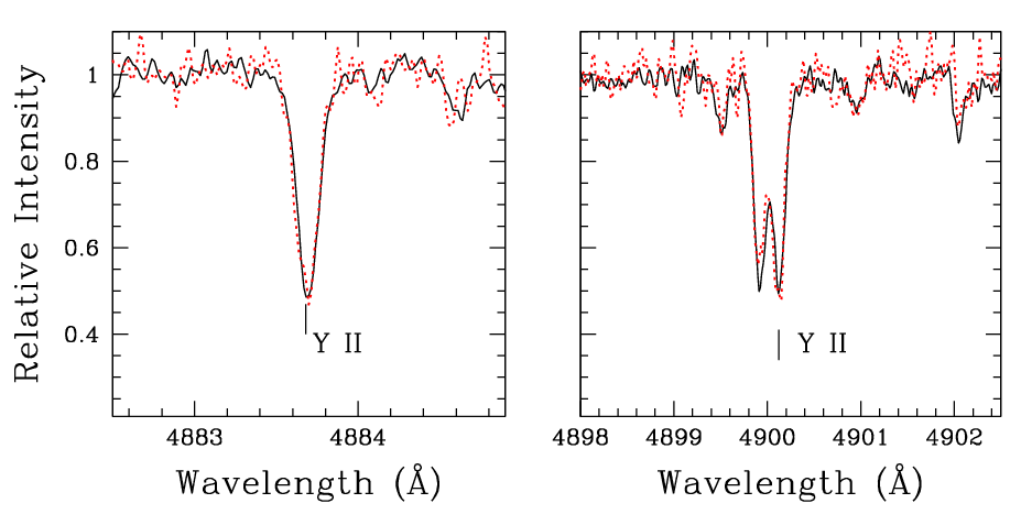
There are no obvious explanations for the origin of this difference since we used the same spectra, the same Y ii line at 4900Å, model atmospheres, and stellar parameters (all from Ma08), as well as the same abundance code, employing the spectral synthesis technique. In Figure 6 we show the direct comparison of the spectra for two stars with very similar atmospheric parameters, and for which VG11 have derived a difference in the [Y/Fe] ratios of [Y/Fe]=0.27, being [Y/Fe]=0.17 for #29848 and [Y/Fe]=0.44 for #26794. As can be seen from the figure, the Y ii lines are of the same strength in both stars and we indeed obtained [Y/Fe]=0.430.11 and [Y/Fe]=0.490.10, respectively. Furthermore, the low [Y/Fe] ratios derived by VG11 for FG stars (ranging from 0.07 to 0.29) does not fit the global picture of the neutron-capture element abundances in M4. In fact, it is well assessed from several studies that M4 is characterised by an intrinsically high -process element content, compared to other GCs (like e.g., its twin M5, see Brown & Wallerstein 1992; Ivans et al. 1999, 2001; Yong et al. 2008a,b; Ma08; Smith 2008; D’Orazi et al. 2010).
On the other hand, five of the stars in our sample are in common with Yong et al. (2008a). The average [Y/Fe] in Yong et al. (2008a) and in our study is 0.690.02 and 0.420.01 dex, respectively, with a difference of 0.27 dex. Such a difference is mainly due to a [Fe/H] offset of 0.180.02 dex, whereas the average [Y/H] values differ only by 0.080.02 dex, within the observational uncertainties in the adopted stellar parameters. For instance, values of Yong and collaborators are on average cooler than Ma08 and log are systematically lower by 0.430.07.
| Star | [Rb/Fe] | Internal |
|---|---|---|
| error | ||
| 28356 | 0.35 | 0.10 |
| 29693 | 0.27 | 0.12 |
| 30711 | 0.35 | 0.10 |
| 30751 | 0.36 | 0.11 |
| 32317 | 0.34 | 0.10 |
| 36215 | 0.32 | 0.12 |
For 6 stars we derived an average value of [Rb/Fe]=0.340.01. Although based on a quite limited sample, the Rb abundance is constant within M4, confirming previous findings by Yong et al. (2008b). One of our star is in common with that study: #36215 (L3624 in Yong et al.’s sample) for which we derived [Rb/H]=0.79 to be compared with [Rb/H]=0.89 by Yong et al. In general there is a good agreement between the two estimates: our mean value is [Rb/H]=0.770.04 (rms=0.09), to be compared to [Rb/H]=0.840.03 (rms=0.09) (see Figure 7).

4 Discussion
M4 is perhaps the most extensively studied GC. Mainly thanks to its close distance (RSun=2.2 kpc, Harris 1996), a wealth of spectroscopic studies have been accomplished, aimed at deriving information on its abundance pattern for species from Li up to Pb. This cluster represents an excellent example of what we deem as an archetypal GC, because it presents substantial changes only in p-capture elements, while heavy elements do not show any variations beyond what is expected from observational errors. A further confirmation of the “standard” nature of M4 can also be found in the recent survey by Carretta et al. (2012a,b), who performed a careful analysis of the Al content in three GCs. In NGC 6752 and 47 Tuc (NGC 104) at least three episodes of star formation are required to account for the chemical pattern. In M4 the classical picture of a FG plus a SG formed from the ejecta (diluted to a certain extent) of FG stars is able to reproduce the observed trends. It is worth mentioning, in this context, that the cluster is however characterised by an intrinsically high level of -process elements, when compared to other clusters like M5 (which has a very similar metallicity, [Fe/H]1.2 dex; see e.g., Ivans et al. 1999, 2001). Several studies have been devoted to assess this very peculiar heavy element pattern, indicating that the proto-cloud from which M4 formed must have been enriched by an higher concentration of -process elements (Yong et al. 2008a).
In the following Section 4.1 we briefly overview the current knowledge of the chemical composition of this cluster. In Section 4.2 we present a new set of intermediate-mass AGB models and discuss their comparison with the observational data to challenge the IM-AGB pollution scenario.
4.1 The chemical abundance pattern of M4
Light elements

The most recent abundance determinations for the key elements Na, O, Mg, Al were presented by Ma08, Carretta et al. (2009a,b) and VG11. Ma08 analysed a sample of 104 giants from high-resolution UVES spectra and detected a well defined Na-O anticorrelation (left panel of Figure 8), with [O/Fe] ranging from 0.20 to 0.55 (=0.35 dex) and [Na/Fe] ranging from 0.05 to 0.53 dex (=0.58 dex). Very similar results were obtained by VG11, who confirmed 0.10[O/Fe]0.53 and 0.11[Na/Fe]0.57, while slightly larger variations in the Na-O plane were measured by Carretta et al. (2009b). Based on the intermediate-resolution FLAMES-Giraffe (R20000) spectra of 88 giants, and a different temperature scale based on photometry, they found the [O/Fe] ratio varying from 0.15 to 0.45 (=0.60 dex) and [Na/Fe] from 0.16 to 0.70 dex (i.e., =0.86 dex). While all the three works detected the presence of a very clear Na-O anticorrelation, there is no consensus on Al. Ma08 found a variation in [Al/Fe] (at 0.4 dex), positively correlated with Na, as also previously detected by Ivans et al. (1999), but no significant (anti)correlation with the Mg abundances. At variance with that study, both Carretta et al. (2009a) and VG11 did not detect any significant variation in the Al content of the cluster (right panel of Figure 8). Carretta et al. presented Mg and Al abundances for a sample of 14 RGB stars from UVES spectra and obtained constant values for [Mg/Fe]=0.550.01 and [Al/Fe]=0.600.01; analogously VG11 found no hint of Al variation, with FG and SG stars showing [Al/Fe]=0.510.04 and [Al/Fe]=0.530.02, respectively. On the other hand, Carretta et al. (2012b) presented Al abundances for 83 RGB stars derived from the strong doublet at 8772-8773Å, properly taking into account the CN features populating that spectral region. They detected a relatively small variation in Al, positively correlated with Na, and confirmed the constancy of the Mg abundances ([Mg/Fe]=+0.5410.005 dex). In general, beyond the debated question of the existence of an Al variation, all these studies agree that the cluster does not show the Mg-Al anticorrelation.
As previously mentioned in Section 1, Li abundances in M4 were derived from three different studies: DM10, Mucciarelli et al. (2011), and VG11. Despite the presence of systematic offsets between the different studies (Li is critically dependent on the adopted effective temperature scale), the main result is that there is no Li-Na anticorrelation and no Li-O correlation (which would be expected in the case of Li destruction within the polluters), since both FG and SG stars show the same Li content. While DM10 and VG11 analysed the Li content in RGB stars (both below and above the RGB bump luminosity), Mucciarelli et al. (2011) gathered Li abundances for a sample of dwarf members, and report A(Li)=2.300.02 dex (rms=0.10), consistent with the Spite plateau defined by halo dwarfs. The fact that FG and SG stars exhibit the same Li calls for yields from the polluters to be at roughly the Spite plateau level and led DM10 to speculate that relatively low-mass polluters (4 M⊙) were at work in M4. Further support to this suggestion comes from the modest Na-O anticorrelation (with the absence of extremely O-poor stars, as compared to other GCs, such as NGC 2808, Bragaglia et al. 2010) and from the lack of the Mg-Al anti-correlations (see, however, the next Section for comparison between models and observations).
Concerning the C and N abundances, the cluster is known to exhibit a very well defined bimodal distribution in the CN band strengths, as first discovered by Norris (1981). Ivans et al. (1999) found that variations in CN are not random but they are positively correlated with Na and Al (with the CN-strong stars showing also higher abundances of Na and Al) and anticorrelated with O. A similar result was later presented by Ma08 who, adopting the CN strength index S(3839) as given by Smith & Briley (2005), showed the (anti)correlation of CN index with (O)Na (see Figure 10 of that paper). The sum of C+N+O has been found to be constant, within the uncertainties, by Ivans et al. (1999) and VG11, who obtained A(C+N+O)=8.240.03 and A(C+N+O)=8.160.02, respectively. We note, in passing, that the constancy of the C+N+O sum in GCs is currently debated. A most striking case is NGC 1851, for which Yong (2011) detected an huge spread of about 1.6 dex11 1 , while Villanova et al. (2010) claimed a constant value.
Finally, the He content has been measured for six blue HB stars from Villanova et al. (2012), who found these stars all enhanced in He by 0.04 dex with respect to the primordial He abundance (i.e., Y=0.24-0.25). The same stars are also Na-rich (O-poor), as expected according to the multiple population scenario (we refer the reader to Gratton et al. 2010 and Marino et al. 2011 for a discussion on the relationship between light-element variations, HB morphology, and the second-parameter problem).
Heavy elements

Yong et al. (2008a,b) published a comprehensive abundance study for a sample of twelve RGB stars in M4, deriving abundances for 27 elements, from Si to Hf. These authors concluded that there is no change in any of the -capture elements under scrutiny; regarding Y they found a mean value of [Y/Fe]=0.690.02 (rms=0.05). The FG stars (i.e., [Na/Fe]0.30) exhibit [Y/Fe]=0.670.03 (rms=0.05) while Na-rich, SG stars have [Y/Fe]=0.700.02(rms=0.06). The Pearson’s correlation coefficient between [Y/Fe] and [Na/Fe] is very small, showing that there is no statistically significant relationship between the two. Similarly, none of the other heavy elements show any significant variation, with [Sr/Fe]=0.730.04, [Zr/Fe]=0.480.03 (from Zr ii lines), [La/Fe]=0.480.03, [Eu/Fe]=0.400.03, and [Pb/Fe]=0.300.02 dex.
Barium abundances were published by Ivans et al. (1999), Ma08, D’Orazi et al. (2010), and VG11 who found [Ba/Fe]=0.600.02, [Ba/Fe]=0.410.01, [Ba/Fe]=0.500.01, and [Ba/Fe]=0.320.02, respectively. We show in Figure 9 the [Ba/Fe] ratio as function of the [Na/Fe] ratio, reporting measurements from these previous studies. Although the Ba abundances are characterised by relatively large uncertainties (due to the saturated behaviour of the Ba ii lines), there is no obvious relationship with the Na abundances (nor with other p-capture elements).
A key element in this context is Rb (=37), whose abundance in the solar system material is 50% -process (Simmerer et al. 2004). Theory predicts that AGB stars with 5M⊙ overproduce Rb with respect to solar and the other nearby -process elements (e.g., Y, Zr). This is the result of neutron densities reaching up to 1014 n/cm3 and favouring the operation of the branching points on the -process path at 85Kr and 86Rb (Abia et al. 2001; van Raai et al. 2012). As previously mentioned in Section 3, Yong et al. (2008a) obtained that the Rb content does not show any cosmic star-to-star scatter (i.e., [Rb/Fe]=0.390.02, rms=0.07). For FG and SG stars, the average ratios are [Rb/Fe]=0.370.02 (rms=0.04) and [Rb/Fe]=0.400.02 (rms=0.07), respectively. We confirm this previous finding and find a mean abundance of [Rb/Fe]=0.340.01.
In summary, all the previous surveys on heavy-element element abundances in M4, with the exception of Y by VG11, agree that these elements do not show any intrinsic inhomogeneity, within the observational uncertainties. This demands that the polluters must account for changes in p-capture elements without affecting the n-capture elements (see Section 4.2).
Finally, since it is not the goal of this paper to discuss the intrinsic enrichment of heavy elements in M4 and to address the origin of the first generations of stars responsible for such a peculiar signature, we refer to previous papers available in the literature on this topic (e.g., Yong et al. 2008a,b; Karakas et al. 2010). We simply take these abundances of light and heavy elements as initial composition and conditions to study the chemical enrichment inside M4 (see section 4.2).
4.2 Intermediate-mass AGB models
4.2.1 The stellar models
| LABEL | Initial Mass | AGB Mass-loss | Ne Rates | No. TPs | Final | |
| STD5 | 5.0 | Vassiliadis & Wood (1993) | 1.75 | Standard | 79 | 0.91 |
| MLT5 | 5.0 | Vassiliadis & Wood (1993) | 2.20 | ” | 73 | 0.91 |
| BLK5 | 5.0 | Bloecker (1995) | 1.75 | ” | 39 | 0.91 |
| M+B5 | 5.0 | Bloecker (1995) | 2.20 | ” | 29 | 0.91 |
| STD6 | 6.0 | Vassiliadis & Wood (1993) | 1.75 | ” | 76 | 1.00 |
| MLT6 | 6.0 | Vassiliadis & Wood (1993) | 2.20 | ” | 55 | 0.99 |
| BLK6 | 6.0 | Bloecker (1995) | 1.75 | ” | 47 | 0.99 |
| M+B6 | 6.0 | Bloecker (1995) | 2.20 | ” | 32 | 0.99 |
| MBR | 6.0 | Bloecker (1995) | 2.20 | 22Ne(p,)23Na higha | 32 | 0.99 |
| & 23Na(p,)24Mg lowa | ||||||
| aAs given by Iliadis et al. (2010). |
We have computed a grid of stellar models to investigate the scenario where the material that went into forming the second generation stars is assumed to come from the ejecta of a population of IM-AGB stars. To compute the stellar structure models we used the Monash version of the Monash-Mount Stromlo evolutionary code (MONSTAR, see eg. Wood & Zarro 1981; Lattanzio 1986; Frost & Lattanzio 1996) including recent updates as described by Campbell & Lattanzio (2008). Low-temperature opacities have been further updated to those calculated by Lederer & Aringer (2009), which are variable in C and N as needed to follow the pollution of the stellar surface via the third dredge-up (TDU) episodes in AGB stars (Marigo, 2002). Instantaneous mixing was used in convective zones and the convective boundaries were defined using a search for “convective neutrality” (Frost & Lattanzio, 1996). No further overshoot was applied beyond this boundary. Initial composition for the models was based on the observed FG abundances reported by VG11 (see their Table 2). This composition is alpha-enhanced and has sub-solar C/Fe. Since the initial [O/Fe] , the metallicity Z is roughly doubled from that given by [Fe/H] only and the present models have initial Z . In our standard models mass-loss was included using the empirical formula of Reimers (1975) during the RGB phase (with ) and the empirical formula of Vassiliadis & Wood (1993) during the AGB phase. The stellar evolution was followed from the zero-age main sequence to the end of the thermally-pulsing AGB phase. In some cases the evolution could not be followed past the instability caused by the peak in Fe opacity in the AGB envelope (see Lau et al. 2012 for a discussion) and final envelope masses between 0.1 and 1.2 remained at the end of the calculations. In these cases when calculating the yields we assume that the surface abundances in this remaining material stay the same as those in the last computed model.
Models of AGB stars are well known to contain many significant uncertainties. These include, but are not limited to: (1) the convection theory, in these models we used the mixing length theory (MLT), (2) the mass-loss rates, and (3) the nuclear reaction rates. Our grid of models explores the effects of these three uncertainties. We calculated two ‘standard’ (STD) models of initial masses 5 M⊙ and 6 M⊙ using the input physics described above and setting the mixing length parameter (where is the mixing length and is the pressure scale-height) to 1.75, as calibrated using a model of the Sun. As a first test, we increased to 2.20. Variations of to this extent are warranted since probably changes for different evolutionary phases (Lydon et al., 1993; Lebzelter & Wood, 2007) and metallicities (Chieffi et al., 1995; Palmieri et al., 2002; Ferraro et al., 2006; Trampedach & Stein, 2011) and it is expected to change for AGB stars (Sackmann & Boothroyd, 1991; Lebzelter & Wood, 2007). Ventura & D’Antona (2005a) found that the value corresponding to employing the full spectrum of turbulence formalism (FST, Canuto & Mazzitelli 1991) in massive AGB stars is 2 (although this does not reproduce all the features of FST models). McSaveney et al. (2007) used values of up to 2.6 to match observations of the effective temperature of the envelopes of massive AGB stars in the Magellanic Clouds. As a second test, we used the mass-loss formula of Bloecker (1995), with during the AGB phase. This mass-loss prescription gives higher mass-loss rates than the formula of Vassiliadis & Wood (1993), effectively reducing the lifetime of the star. The star consequently suffers fewer thermal pulses and therefore fewer TDU episodes, which follow each TP (see also Ventura & D’Antona 2005b). As a third test, we changed both the mass-loss rate to Bloecker (1995) and to 2.2.
We also performed detailed nucleosynthesis calculations using a post-processing code, the Monash Stellar Nucleosynthesis code (MONSOON; Cannon 1993; Lattanzio et al. 1996; Lugaro et al. 2004), that reads as input the background thermal structure from the stellar evolution calculations. The code solves a network of 2,336 nuclear reactions involving 320 nuclear species from n and p up to Bi. The bulk of the reaction rates are from the JINA reaclib database as of May 2009. We tested that there are no major changes when using the database as of May 2012. During the post-processing we made one final test to investigate the effects of changing the p-capture rates that affect the production of 23Na, as detailed in the last line of Table 4 (model MBR, see also Ventura & D’Antona 2005b; 2006). We summarise the 9 computed models and their parameters in Table 4.
4.2.2 Model results
In the last two columns of Table 4 we list the total number of thermal pulses and the final core mass for each model. The models show little difference in final core mass because the core grows very slowly due to the presence of deep TDU episodes, which removes the core growth due to H burning (i.e., ). The mass of the core is not affected by higher mass-loss rates since it essentially reaches its final value after 10 TPs. On the other hand, the different models present large differences in the number of TPs. Increasing caused a minor reduction in number of TPs in the 5 M⊙ model while in the 6 M⊙ model the number of TPs was reduced by . This is a result of hotter HBB and higher luminosities driving an enhanced mass loss (Ventura & D’Antona, 2005a). In the models with increased mass-loss rates, due to the use of the Bloecker (1995) formula, obviously the effect is stronger. In both the 5 M⊙ and 6 M⊙ models the number of TPs as compared to the standard models is significantly lower, reducing from TPs and TPs, respectively. As expected, the combination of a higher and a higher mass-loss rate leads to an even further reduction of the number of TPs (Table 4).


In Figures 10 and 11 we compare the evolution of the surface abundances along the AGB in the standard 6 M⊙ model (STD6) and in the 6 M⊙ model computed using Bloecker mass-loss and (M+B6). Using the formula of Bloecker (1995) and severely truncates the AGB phase, resulting in fewer TDU episodes and less material carried into the envelope. The abundances of species arising from the TDU are lower, e.g., the sum of C+N+O (Figure 10) and the -process elements (Figure 11). The sum of C+N+O is determined by the amount of C produced by He burning during the TPs, dredged-up to the stellar surface, and partially converted to N by HBB. Thus, the truncation of the AGB phase naturally leads to a significantly smaller increase in the sum of C+N+O. The higher value of also has the effect of decreasing the number of TDU episodes and, in addition, it has the important consequence of altering the thermal structure of the convective envelope. In particular, the temperature at the base of the envelope increases. This allows more efficient HBB, which modifies the nucleosynthetic yields of all the species affected by proton captures, for example, the surface O abundance reduces faster (Figure 10).
The -process elements in our IM-AGB star models are produced in the convective regions associated with the TPs. The neutron source during the TPs is the 22Ne(,n)25Mg reaction. The 22Ne is synthesised in the TPs by conversion of all the 14N, produced by the H-burning shell during the interpulse period, via two captures. An important fraction of the 22Ne abundance is of primary origin since it is formed from 14N which is produced via proton captures on the 12C left behind by He burning and carried to the envelope by the TDU. The other possible neutron source in AGB stars is the 13C(,n)16O reaction. Formation of the required 13C is usually obtained by allowing some extra mixing of protons at the deepest extent of the convective envelope during each TDU episode (Busso et al., 1999). However, we did not include the 13C pocket in our models because in IM-AGB stars the formation of the 13C pocket appears to be inhibited by p captures occurring at the hot base of the convective envelope during the TDU (Goriely & Siess, 2004). The surface -process abundances increase with each TDU episode as they are successively mixed into the convective envelope (see Figure 11). The activation of the 22Ne neutron source depends on the temperature at the base of the TP convection zone, which increases with each TP. Because the -process nuclei accumulate in the He intershell and are irradiated during each TP, they experience a total neutron flux that increases with the TP number. As a result, the -process surface abundances show an increase initially of the elements at the first -process peak (Rb, Sr, Y, and Zr), then of the elements at the second peak (e.g., Ba), and finally of those of the third peak at Pb. The -process elements belonging to the same neutron magic peak (e.g., Sr, Y and Zr, N = 50) are produced together along the -process path, according to the local neutron capture rates. In Figure 11 we show the production of heavy elements for two 6 M⊙ AGB models (standard case and enanched+Bloecker mass-loss law). For the first model, [Rb/Fe] increases up to 1.4 dex, Sr-Y-Zr up to 1.1 dex [Ba/Fe] up to 0.7 dex and Pb only marginally changes, growing less than 0.2 dex. In the second model, the -process production is much weaker, since all elements under consideration have abundances lower than roughly 0.5 dex. To explain variations in only one of these elements (eg., Y, as reported by VG11) would require very unusual conditions. The production of Rb with respect to solar is higher than the production of Y, due to the high neutron densities resulting from the activation of the 22Ne neutron source (van Raai et al., 2012).
4.2.3 Comparison with observations of M4
In Figures 13 to 21 we compare the elemental yields in the form of [X/Fe] predicted by the present models with the key abundances observed in M4. The “yields” are defined as the integrated elemental abundance lost in the AGB winds during the whole life of the star. This is the material that presumably contributes to the gas from which the SG stars formed.
- -
Na and O: In Figures 13 and 13 we present the comparison between models and observations in the Na-O plane for the 5 M⊙ and 6 M⊙ models, respectively. It can be seen that the MLT5 model covers the range of Na increase and O decrease, while the other 5 M⊙ models fail to deplete O sufficiently. On the other hand, most of the 6 M⊙ models deplete enough O, but fail to produce significant amounts of Na. The MBR model, computed by altering the p-capture reaction rates that affect the Na abundance (within the uncertainties given by Iliadis et al. 2010), results in a Na yield 70% higher than using the recommended rates. This is not enough to match the observed variation between the FG and SG stars, however, it should be considered as a conservative choice. Iliadis et al. (2010) provided new estimates for nuclear reaction rates based on a Monte Carlo model that allowed the evaluation of the probability distribution function for each rate. They defined as “low” and “high” those rates corresponding to a coverage probability of 1 – clearly the uncertainties would be larger if one adopted a higher coverage probability. Also, it should be noted that while the Monte Carlo method takes into account all current experimental information, it cannot be excluded that different information may arise from future experiments, particularly for the 22Ne(p,)23Na and 23Na(p,)24Mg rates, which are affected by low-energy resonances that are difficult to reach experimentally.

Figure 12: Comparison between our 5 M⊙ model yields and observations in the O-Na plane (as in Figure 8). Large markers indicate yields from models as indicated in the figure (see Table 4), except for the solid diamond which shows the initial composition. Observational data are from the same sources as in Figure 8. 
Figure 13: Same as Figure 13 except for the 6 M⊙ models. - -
Mg and Al: In Figures 15 and 15 we present the comparison between models and observations in the Mg-Al plane for the 5 M⊙ and 6 M⊙ models, respectively. The STD and MLT models produce Mg and/or Al abundances too high with respect to the observations, either due to dredge-up of 25,26Mg produced by captures on 22Ne, in the case of the 5 M⊙ models, or due to efficient HBB in case of the 6 M⊙ models. On the other hand, all the BLK and M+B models are well within the observations (we remind the reader that the extent of the Al spread is debated, as described in detail in Section 4.1).
- -
Na and Y: In Figures 17 and 17 present the comparison between models and observations in the Na-Y plane for the 5 M⊙ and 6 M⊙ models. The STD and MLT models, which experience a large number of TDU episodes, produce Y variations an order of magnitude higher than the spread observed in M4. Therefore, within the IM-AGB pollution scenario these models would cause a larger s-process enrichment in SG stars compared to FG stars, which is not observed according also to our present results. On the other hand, the BLK and M+B models, which experience fewer TDU episodes, produce Y variations of and 0.2 dex for the 5 M⊙ and 6 M⊙ models respectively. These models may reproduce better the observations, i.e., the missing extra-enrichment in -process elements of SG stars compared to FG stars in M4 within the uncertainties. A similar conclusion can be derived using the Na-Ba plane (Figures 19 and 19).
- -
Li: Figures 21 and 21 show the comparison between models and observations in the Teff-Li plane for the 5 M⊙ and 6 M⊙ models. All our models present a brief phase of Li enrichment at the stellar surface, during the first few TPs, with a peak of A(Li)4 dex. The final Li yield depends on when the star loses most of its mass (Travaglio et al. 2001; Ventura & D’Antona 2010). The STD and MLT models, which experience extended lifetimes, result in yields close to zero, because they lose most of their mass after Li has been destroyed by HBB. Conversely, the BLK and M+B models, which have shorter lifetimes, eject a substantial amount of mass during their Li-rich phases, producing relatively high yields – close to the initial value – particularly when considering the 5 M⊙ model.


Overall, none of our STD and MLT models can reproduce the observed constancy in the -process and Li abundances. Furthermore, they produce Mg and Al outside the observed variations. On the other hand, the BLK and M+B models can reproduce most of the observational constraints, although the 5 M⊙ models do not deplete enough O and result in slightly too high -process abundances, while the 6 M⊙ models require some adjustment in the reaction rates to explain the Na spread, and they deplete too much Li. The Li problem might be rectified by a further slight increase in mass-loss rate, for instance using a slightly higher value of in the Bloecker formula, so that more mass is lost during the Li-rich phase, and/or by considering in detail the uncertainties in the nuclear reaction rates involved.
Finally, we report that in the M+B6 model the [Rb/Fe] increases of +0.2 dex, slightly higher than that predicted for [Y/Fe]. However, this is not a problem since such a weak overall enrichment of Rb and Y in these IM-AGB models as polluters would likely not be observable in SG stars. For the same model, the change in the sum of C+N+O is +0.3 dex, and the He enrichment is Y . All the models produce [N/Fe] 1.5-2 (the observed variation is up to 1 dex; e.g., VG11), but none of them deplete C to the observed level of [C/Fe]0.5 (e.g., VG11). The lowest [C/Fe] obtained is 0 using the M+B6 model.
4.2.4 Comparison with other observational constraints
To ascertain if our IM-AGB models computed including efficient HBB and strong mass loss are a realistic solution for the anomalies observed in M4 we can, in principle, check if these models are consistent with other observational constraints. A problem however is that there are very few direct observations of abundances in IM-AGB stars, and these are for stars in the Galaxy, LMC, or SMC, i.e., of metallicities higher than M4. One study that we are aware of is that of McSaveney et al. (2007), who obtained spectra of a sample of LMC and SMC AGB stars. The severe difficulties in performing these observations are clear from the McSaveney et al. (2007) study, where they attempted to measure abundances in the cool AGB atmospheres (which are also dynamic/pulsating, see e.g., Lebzelter et al. 2010) of 7 stars but were only able to obtain results for two. The results from their two stars support an increase in at least as high as we have used in our MLT models and also the phenomena of HBB and TDU as seen in the models. Other studies of IM-AGB stars are those of Plez et al. (1993) for the Small Magellanic Cloud (SMC), and those of García-Hernández et al. (2006, 2007, 2009) discussed below, for the Galaxy, the SMC and the Large Magellanic Cloud (LMC). More accessible are planetary nebulae (PNe) of Type I. The material surrounding the compact central stars in these objects is believed to consist of the material ejected by IM-AGB stars. They are also located in the Galactic disk (Stanghellini et al., 2006; Sterling & Dinerstein, 2008), or in the LMC and SMC (Kaler & Jacoby, 1990). Again, all these objects have metallicities higher than M4, which may affect the uncertain parameters related to the evolution of these stars. Keeping this caveat in mind, we can examine the available constraints.
Planetary nebulae (PNe) of Type I are believed to be IM stars that have completed the AGB phase, have little or no stellar envelope left, and are evolving blue-wards at constant luminosity in the CMD. PNe of Type I show the clear signature of HBB in their He/H and N/O ratios (e.g., Kaler & Jacoby 1990; Stanghellini et al. 2006) and no enhancements of the -process elements Se and Kr, which are close to the first -process peak. This is well explained by models of IM-AGB stars of solar metallicity (Karakas et al., 2009). However, this simple picture has been somewhat complicated by the detection of extremely high abundances of Rb in OH/IR stars in the Galaxy (García-Hernández et al., 2006), and in the SMC/LMC (García-Hernández et al., 2009), which represents the first proof of the activation of the 22Ne neutron source in IM-AGB stars. The IM-AGB nature of these stars was determined on the basis of the velocities of their OH masers, their location in the Galactic plane (as indicative of belonging to a young population), and the presence of Li produced by HBB, at least in some of the objects. The very high Rb overabundances, with [Rb/Fe] up to +2.5 dex for Galactic stars and up to +5 dex for stars in the Magellanic Clouds are however not matched by standard IM-AGB models (García-Hernández et al., 2009; van Raai et al., 2012). Karakas et al. (2012) showed that if the stellar lifetime is extended by lowering the mass-loss rate, so that a larger number of TDUs is allowed, and the rate of the 22Ne(,n)25Mg reaction is taken from the NACRE compilation (Angulo et al., 1999), then it is possible to reach [Rb/Fe] , close to the average [Rb/Fe] observed in the Galactic OH/IR stars. Clearly, we have here a contradictory situation since to match these observations the -process nucleosynthesis in IM-AGB stars needs to be enhanced, while to match the constancy of the -process elements in M4, including Rb, the -process nucleosynthesis in IM-AGB stars needs to be suppressed.
We note however that there are still several problems related to the interpretation of the high Rb abundances in IM-AGB:
- 1.
as discussed in detail by García-Hernández et al. (2009) and van Raai et al. (2012), serious problems are present in current model atmospheres of luminous AGB stars since these models are performed in 1D and do not include important effects such as the presence of a circumstellar dust envelope and dust formation, which may lead to systematic uncertainties. More realistic model atmospheres for intermediate-mass O-rich AGB stars (e.g., the inclusion of a circumstellar dust envelope and 3D hydrodynamical simulations, see e.g., Lebzelter et al. 2010) as well as NLTE calculations need to be developed;
- 2.
the IM-AGB models that predict high Rb enhancements also necessarily predict some Zr enhancements, which are not observed. These stars show [Zr/Fe] (García-Hernández et al., 2007);
- 3.
the NACRE 22Ne(,n)25Mg rate is probably too high when considering the more recent experiments (Jaeger et al., 2001);
- 4.
Li abundances in the observed stars present a large range, from depletion to enhancements, however (as also discussed above in relation to the present models), Li enhancements can only be seen early during the AGB evolution, while high Rb enhancements are obtained only after many TPs.
Another possibility is that the TDU efficiency and the mass-loss rate are very sensitive to the initial stellar mass and the metallicity. For example, more massive IM-AGBs than those considered here and Super-AGB stars (Pumo et al. 2008, Doherty et al. 2010, Siess 2010) might experience less efficient TDU and/or higher mass-loss rates and be responsible for the pollution of GCs. Obviously, more models of IM-AGB stars and observations of both Rb-rich stars and Type I PNe will help us to understand these issues. For the time being it seems difficult to use the high-Rb observations as a strong constraint to extrapolate information to IM-AGB stars in GCs and viceversa.
A further difficulty when comparing to other observational constraints is the possibility that IM-AGB stars could evolve differently in clusters and in the field. It is known that B stars (which eventually evolve to be IM-AGB stars) in open clusters typically rotate more rapidly than B stars in the field (though this may be due to their being in a less evolved phase of their evolution, e.g., Huang et al. 2010). Fast rotation would have a strong effect on the stellar evolution prior to the AGB phase possibly producing too high C+N+O yields to be compatible with the observations, as shown by Decressin et al. (2009), though the effect of magnetic fields was not included in these models. Moreover, binary interaction is important in shaping stellar yields (Izzard et al. 2006, Vanbeveren et al. 2012) and its effects would be different if the binary distribution was different for field and cluster stars.
5 Summary and concluding remarks
In summary we have considered four observational constraints and derived the following results for M4:
- 1.
In the O-Na plane, the MLT5 model provides a good fit to the observed spread. Also the STD6 and the M+B6 models may result in a good fit, provided that the rates of the nuclear reaction that produce and destroy Na during HBB are varied somewhat beyond the ‘high’ and ‘low’ values given by Iliadis et al. (2010). These variations are within current possibilities and need to be investigated.
- 2.
In the Mg-Al plane, all the STD and MLT models produce variations in Mg and/or Al outside the observed spread, while all the BLK and M+B models are within the observations.
- 3.
As in item (ii), in the Na-Y and Na-Ba planes the STD and MLT models produce variations outside the observed spread, while the BLK and M+B models can explain the constancy of -process abundances between generations, particularly when considering the 6 M⊙ models.
- 4.
As in items (ii) and (iii), when considering Li the STD and MLT models result in no Li production, while the BLK and M+B models can explain the constancy of the Li abundance between generations, particularly when considering the 5 M⊙ models.
- 5.
All the models result in production of He beyond the observed variations, which indicates the need of some dilution with primitive material. The change in the sum of C+N+O may be comparable to the observations, within the uncertainties, only if we consider the BLK and M+B models. The observed depletion of C by a factor 2 is not obtained by any of the models.
Although none of these models can simultaneously match all the constraints listed above, we believe that our exploration of the model uncertainties shows that IM-AGB stars cannot be ruled out as potential polluters for the M4 SG population since reasonable variations in input physics can still provide a reasonable agreement between the theoretical yields and observations. More work is clearly needed to improve the input physics of IM-AGB stars. We note, however, that the fact that SG stars probably formed from the ejecta of a range of masses (not a single mass) and that there must be a certain dilution between pristine and polluted material (see e.g., Gratton et al. 2012), do not allow us to simultaneously reproduce all the observational constraints any better with the present models.
We have confirmed the previous finding by Ventura & D’Antona (2005c; 2010) that IM-AGB models computed including efficient HBB and strong mass loss (e.g., the Bloecker mass-loss rate) can provide a match to the observations of the light elements. Furthermore, we have shown that these same models can also be consistent with the constraint that there are no variations in the -process elements in M4 between FG and SG. When comparing to observational constraints other than GCs, however, it appears difficult to establish a self-consistent scenario that could explain all the current observations related to IM-AGB stars. Also the question remains of why IM-AGB stars in GCs should experience a stronger mass loss than what is observed in the Galaxy and in the Magellanic Clouds (Vassiliadis & Wood, 1993). In any case, pursuing such comparison offers us the future opportunity of better understanding all of the current issues related to nucleosynthesis in IM-AGB stars via more refined models and observations.
In particular, AGB -process models similar to those we have explored here are needed for a more extended range of masses, i.e., between 3 M⊙ and 9 M⊙, and for different choices of the mass-loss rate and efficiency of convection. The models of Lugaro et al. (2012) have shown that as the stellar mass decreases the effect of the TDU (producing C, F, and -process elements) gradually becomes predominant over the effect of HBB (depleting O, and F, and producing Li). AGB models of slightly lower mass than those presented here have been invoked as a possible explanation for variations in the -process elements in M22 (Roederer et al. 2011, Marino et al. 2009), as well as for their correlation with fluorine (D’Orazi et al. 2013). A large grid of AGB models and realistic models of the gas dynamics in the forming GC (Krause et al. 2012,2013) will be fundamental to ascertain at which mass we can see the raising of the -process and fluorine abundances, and to derive information on the timescales of formation of the different populations in GCs.
Acknowledgments
The authors warmly thank the referee for a very careful reading of the manuscript and for valuable comments and suggestions. This work made extensive use of the SIMBAD, Vizier, and NASA ADS database. We acknowledge B. Plez for providing his unpublished line lists. We thank F. D’Antona, T. Decressin, C. Doherty, A. García-Hernández, A. I. Karakas, G. Imbriani, A.F. Marino, M. Wiescher for helpful discussions and C. Iliadis for detailed explanation of reaction rate uncertainties. ML is supported by an ARC Future Fellowship and a Monash Fellowship. SWC is supported by an Australian Research Council Discovery Project grant (DP1095368). MP thanks support from an Ambizione grant of the SNSF (Switzerland), and from EuroGENESIS (MASCHE).
References
- Abia et al. (2001) Abia C., Busso M., Gallino R., Domínguez I., Straniero O., Isern J., 2001, ApJ, 559, 1117
- Angulo et al. (1999) Angulo C. et al., 1999, Nuclear Physics A, 656, 3
- Armosky et al. (1994) Armosky B. J., Sneden C., Langer G. E., Kraft R. P., 1994, AJ, 108, 1364
- Asplund et al. (2009) Asplund M., Grevesse N., Sauval A. J., Scott P., 2009, ARA&A, 47, 481
- Bloecker (1995) Bloecker T., 1995, A&A, 297, 727
- Bragaglia et al. (2010) Bragaglia A. et al., 2010, ApJL, 720, L41
- Brown & Wallerstein (1992) Brown J. A., Wallerstein G., 1992, AJ, 104, 1818
- Busso et al. (1999) Busso M., Gallino R., Wasserburg G. J., 1999, ARA&A, 37, 239
- Cameron & Fowler (1971) Cameron A. G. W., Fowler W. A., 1971, ApJ, 164, 111
- Campbell & Lattanzio (2008) Campbell S. W., Lattanzio J. C., 2008, A&A, 490, 769
- Cannon (1993) Cannon R. C., 1993, MNRAS, 263, 817
- Canuto & Mazzitelli (1991) Canuto V. M., Mazzitelli I., 1991, ApJ, 370, 295
- Carretta et al. (2009a) Carretta E., Bragaglia A., Gratton R., Lucatello S., 2009a, A&A, 505, 139
- Carretta et al. (2010a) Carretta E., Bragaglia A., Gratton R., Lucatello S., Bellazzini M., D’Orazi V., 2010a, ApJL, 712, L21
- Carretta et al. (2010b) Carretta E. et al., 2010b, A&A, 520, A95
- Carretta et al. (2009b) Carretta E. et al., 2009b, A&A, 505, 117
- Carretta et al. (2010c) Carretta E., Bragaglia A., Gratton R. G., Recio-Blanco A., Lucatello S., D’Orazi V., Cassisi S., 2010c, A&A, 516, A55
- Chieffi et al. (1995) Chieffi A., Straniero O., Salaris M., 1995, ApJL, 445, L39
- Cohen (1999) Cohen J. G., 1999, AJ, 117, 2434
- D’Antona & Ventura (2008) D’Antona F., Ventura P., 2008, in American Institute of Physics Conference Series, Vol. 1001, Evolution and Nucleosynthesis in AGB Stars, Guandalini R., Palmerini S., Busso M., eds., pp. 41–48
- Decressin et al. (2008) Decressin T., Baumgardt H., Kroupa P., 2008, A&A, 492, 101
- Decressin et al. (2007) Decressin T., Charbonnel C., Meynet G., 2007, A&A, 475, 859
- Decressin et al. (2009) Decressin T., Charbonnel C., Siess L., Palacios A., Meynet G., Georgy C., 2009, A&A, 505, 727
- Denisenkov & Denisenkova (1989) Denisenkov P. A., Denisenkova S. N., 1989, Astronomicheskij Tsirkulyar, 1538, 11
- D’Ercole et al. (2010) D’Ercole A., D’Antona F., Ventura P., Vesperini E., McMillan S. L. W., 2010, MNRAS, 407, 854
- D’Ercole et al. (2008) D’Ercole A., Vesperini E., D’Antona F., McMillan S. L. W., Recchi S., 2008, MNRAS, 391, 825
- Doherty et al. (2010) Doherty C. L., Siess L., Lattanzio J. C., Gil-Pons P., 2010, MNRAS, 401, 1453
- D’Orazi et al. (2010) D’Orazi V., Gratton R., Lucatello S., Carretta E., Bragaglia A., Marino A. F., 2010, ApJL, 719, L213
- D’Orazi et al. (2011) D’Orazi V., Gratton R. G., Pancino E., Bragaglia A., Carretta E., Lucatello S., Sneden C., 2011, A&A, 534, A29
- D’Orazi et al. (2013) D’Orazi V. et al., 2013, ApJ, 763, 22
- D’Orazi & Marino (2010) D’Orazi V., Marino A. F., 2010, ApJL, 716, L166
- Fenner et al. (2004) Fenner Y., Campbell S., Karakas A. I., Lattanzio J. C., Gibson B. K., 2004, MNRAS, 353, 789
- Ferraro et al. (2006) Ferraro F. R., Valenti E., Straniero O., Origlia L., 2006, ApJ, 642, 225
- Frost & Lattanzio (1996) Frost C. A., Lattanzio J. C., 1996, ApJ, 473, 383
- Gallino et al. (1998) Gallino R., Arlandini C., Busso M., Lugaro M., Travaglio C., Straniero O., Chieffi A., Limongi M., 1998, ApJ, 497, 388
- García-Hernández et al. (2006) García-Hernández D. A., García-Lario P., Plez B., D’Antona F., Manchado A., Trigo-Rodríguez J. M., 2006, Science, 314, 1751
- García-Hernández et al. (2007) García-Hernández D. A., García-Lario P., Plez B., Manchado A., D’Antona F., Lub J., Habing H., 2007, A&A, 462, 711
- García-Hernández et al. (2009) García-Hernández D. A. et al., 2009, ApJL, 705, L31
- Goriely & Siess (2004) Goriely S., Siess L., 2004, A&A, 421, L25
- Gratton et al. (2004) Gratton R., Sneden C., Carretta E., 2004, ARA&A, 42, 385
- Gratton et al. (2001) Gratton R. G. et al., 2001, A&A, 369, 87
- Gratton et al. (2012) Gratton R. G., Carretta E., Bragaglia A., 2012, A&ARv, 20, 50
- Gratton et al. (2010) Gratton R. G., Carretta E., Bragaglia A., Lucatello S., D’Orazi V., 2010, A&A, 517, A81
- Gratton et al. (2011) Gratton R. G., Lucatello S., Carretta E., Bragaglia A., D’Orazi D’Orazi V., Momany Y. A., 2011, A&A, 534, A123
- Grevesse et al. (1996) Grevesse N., Noels A., Sauval A. J., 1996, in Astronomical Society of the Pacific Conference Series, Vol. 99, Cosmic Abundances, Holt S. S., Sonneborn G., eds., p. 117
- Grevesse & Sauval (1998) Grevesse N., Sauval A. J., 1998, Space Science Reviews, 85, 161
- Harris (1996) Harris W. E., 1996, VizieR Online Data Catalog, 7195, 0
- Huang et al. (2010) Huang W., Gies D. R., McSwain M. V., 2010, ApJ, 722, 605
- Iliadis et al. (2010) Iliadis C., Longland R., Champagne A. E., Coc A., Fitzgerald R., 2010, Nuclear Physics A, 841, 31
- Ivans et al. (2001) Ivans I. I., Kraft R. P., Sneden C., Smith G. H., Rich R. M., Shetrone M., 2001, AJ, 122, 1438
- Ivans et al. (1999) Ivans I. I., Sneden C., Kraft R. P., Suntzeff N. B., Smith V. V., Langer G. E., Fulbright J. P., 1999, AJ, 118, 1273
- Izzard et al. (2006) Izzard R. G., Dray L. M., Karakas A. I., Lugaro M., Tout C. A., 2006, A&A, 460, 565
- Jaeger et al. (2001) Jaeger M., Kunz R., Mayer A., Hammer J. W., Staudt G., Kratz K. L., Pfeiffer B., 2001, Physical Review Letters, 87, 202501
- James et al. (2004) James G., François P., Bonifacio P., Carretta E., Gratton R. G., Spite F., 2004, A&A, 427, 825
- Johnson & Pilachowski (2010) Johnson C. I., Pilachowski C. A., 2010, ApJ, 722, 1373
- Kaler & Jacoby (1990) Kaler J. B., Jacoby G. H., 1990, ApJ, 362, 491
- Käppeler et al. (2011) Käppeler F., Gallino R., Bisterzo S., Aoki W., 2011, Reviews of Modern Physics, 83, 157
- Karakas et al. (2010) Karakas A. I., Campbell S. W., Lugaro M., Yong D., Chieffi A., 2010, Mem. Sait, 81, 1010
- Karakas et al. (2006) Karakas A. I., Fenner Y., Sills A., Campbell S. W., Lattanzio J. C., 2006, ApJ, 652, 1240
- Karakas et al. (2012) Karakas A. I., García-Hernández D. A., Lugaro M., 2012, ApJ, 751, 8
- Karakas et al. (2009) Karakas A. I., van Raai M. A., Lugaro M., Sterling N. C., Dinerstein H. L., 2009, ApJ, 690, 1130
- Kayser et al. (2008) Kayser A., Hilker M., Grebel E. K., Willemsen P. G., 2008, A&A, 486, 437
- Krause et al. (2013) Krause M., Charbonnel C., Decressin T., Meynet G., Prantzos N., 2013, ArXiv e-prints
- Krause et al. (2012) Krause M., Charbonnel C., Decressin T., Meynet G., Prantzos N., Diehl R., 2012, A&A, 546, L5
- Kurucz (1993) Kurucz R., 1993, ATLAS9 Stellar Atmosphere Programs and 2 km/s grid. Kurucz CD-ROM No. 13. Cambridge, Mass.: Smithsonian Astrophysical Observatory, 1993., 13
- Lambert & Luck (1976) Lambert D. L., Luck R. E., 1976, The Observatory, 96, 100
- Lattanzio et al. (1996) Lattanzio J., Frost C., Cannon R., Wood P. R., 1996, Mem.SAIt, 67, 729
- Lattanzio (1986) Lattanzio J. C., 1986, ApJ, 311, 708
- Lau et al. (2012) Lau H. H. B., Gil-Pons P., Doherty C., Lattanzio J., 2012, A&A, 542, A1
- Lebzelter et al. (2010) Lebzelter T., Nowotny W., Höfner S., Lederer M. T., Hinkle K. H., Aringer B., 2010, A&A, 517, A6
- Lebzelter & Wood (2007) Lebzelter T., Wood P. R., 2007, A&A, 475, 643
- Lederer & Aringer (2009) Lederer M. T., Aringer B., 2009, A&A, 494, 403
- Lind et al. (2009) Lind K., Primas F., Charbonnel C., Grundahl F., Asplund M., 2009, A&A, 503, 545
- Lodders & Palme (2009) Lodders K., Palme H., 2009, Meteoritics and Planetary Science Supplement, 72, 5154
- Lugaro et al. (2012) Lugaro M., Karakas A. I., Stancliffe R. J., Rijs C., 2012, ApJ, 747, 2
- Lugaro et al. (2004) Lugaro M., Ugalde C., Karakas A. I., Görres J., Wiescher M., Lattanzio J. C., Cannon R. C., 2004, ApJ, 615, 934
- Lydon et al. (1993) Lydon T. J., Fox P. A., Sofia S., 1993, ApJ, 413, 390
- Marigo (2002) Marigo P., 2002, A&A, 387, 507
- Marino et al. (2009) Marino A. F., Milone A. P., Piotto G., Villanova S., Bedin L. R., Bellini A., Renzini A., 2009, A&A, 505, 1099
- Marino et al. (2011) Marino A. F., Villanova S., Milone A. P., Piotto G., Lind K., Geisler D., Stetson P. B., 2011, ApJL, 730, L16
- Marino et al. (2008) Marino A. F., Villanova S., Piotto G., Milone A. P., Momany Y., Bedin L. R., Medling A. M., 2008, A&A, 490, 625
- McSaveney et al. (2007) McSaveney J. A., Wood P. R., Scholz M., Lattanzio J. C., Hinkle K. H., 2007, MNRAS, 378, 1089
- Mucciarelli et al. (2011) Mucciarelli A., Salaris M., Lovisi L., Ferraro F. R., Lanzoni B., Lucatello S., Gratton R. G., 2011, MNRAS, 412, 81
- Norris (1981) Norris J., 1981, ApJ, 248, 177
- Palmieri et al. (2002) Palmieri R., Piotto G., Saviane I., Girardi L., Castellani V., 2002, A&A, 392, 115
- Pasquini et al. (2002) Pasquini L. et al., 2002, The Messenger, 110, 1
- Pasquini et al. (2005) Pasquini L., Bonifacio P., Molaro P., Francois P., Spite F., Gratton R. G., Carretta E., Wolff B., 2005, A&A, 441, 549
- Pignatari et al. (2010) Pignatari M., Gallino R., Heil M., Wiescher M., Käppeler F., Herwig F., Bisterzo S., 2010, ApJ, 710, 1557
- Plez et al. (1993) Plez B., Smith V. V., Lambert D. L., 1993, ApJ, 418, 812
- Prantzos et al. (1990) Prantzos N., Hashimoto M., Nomoto K., 1990, A&A, 234, 211
- Pumo et al. (2008) Pumo M. L., D’Antona F., Ventura P., 2008, ApJL, 672, L25
- Raiteri et al. (1991) Raiteri C. M., Busso M., Picchio G., Gallino R., 1991, ApJ, 371, 665
- Raiteri et al. (1993) Raiteri C. M., Gallino R., Busso M., Neuberger D., Kaeppeler F., 1993, ApJ, 419, 207
- Ramírez & Allende Prieto (2011) Ramírez I., Allende Prieto C., 2011, ApJ, 743, 135
- Ramírez & Cohen (2002) Ramírez S. V., Cohen J. G., 2002, AJ, 123, 3277
- Rauscher et al. (2002) Rauscher T., Heger A., Hoffman R. D., Woosley S. E., 2002, ApJ, 576, 323
- Recchi & Danziger (2005) Recchi S., Danziger I. J., 2005, A&A, 436, 145
- Reimers (1975) Reimers D., 1975, Memoires of the Societe Royale des Sciences de Liege, 8, 369
- Renzini (2008) Renzini A., 2008, MNRAS, 391, 354
- Roederer (2011) Roederer I. U., 2011, ApJL, 732, L17
- Roederer et al. (2011) Roederer I. U., Marino A. F., Sneden C., 2011, ApJ, 742, 37
- Sackmann & Boothroyd (1991) Sackmann I.-J., Boothroyd A. I., 1991, ApJ, 366, 529
- Shen et al. (2010) Shen Z.-X., Bonifacio P., Pasquini L., Zaggia S., 2010, A&A, 524, L2
- Siess (2010) Siess L., 2010, A&A, 512, A10
- Simmerer et al. (2004) Simmerer J., Sneden C., Cowan J. J., Collier J., Woolf V. M., Lawler J. E., 2004, ApJ, 617, 1091
- Smith (2008) Smith G. H., 2008, PASP, 120, 952
- Smith et al. (2005) Smith V. V., Cunha K., Ivans I. I., Lattanzio J. C., Campbell S., Hinkle K. H., 2005, ApJ, 633, 392
- Smith et al. (2000) Smith V. V., Suntzeff N. B., Cunha K., Gallino R., Busso M., Lambert D. L., Straniero O., 2000, AJ, 119, 1239
- Sneden (1973) Sneden C. A., 1973, PhD thesis, THE UNIVERSITY OF TEXAS AT AUSTIN.
- Stanghellini et al. (2006) Stanghellini L., Guerrero M. A., Cunha K., Manchado A., Villaver E., 2006, ApJ, 651, 898
- Sterling & Dinerstein (2008) Sterling N. C., Dinerstein H. L., 2008, ApJS, 174, 158
- The et al. (2007) The L.-S., El Eid M. F., Meyer B. S., 2007, ApJ, 655, 1058
- Tomkin & Lambert (1999) Tomkin J., Lambert D. L., 1999, ApJ, 523, 234
- Trampedach & Stein (2011) Trampedach R., Stein R. F., 2011, ApJ, 731, 78
- Travaglio et al. (2001) Travaglio C., Randich S., Galli D., Lattanzio J., Elliott L. M., Forestini M., Ferrini F., 2001, ApJ, 559, 909
- van Raai et al. (2012) van Raai M. A., Lugaro M., Karakas A. I., García-Hernández D. A., Yong D., 2012, A&A, 540, A44
- Vanbeveren et al. (2012) Vanbeveren D., Mennekens N., De Greve J. P., 2012, A&A, 543, A4
- Vassiliadis & Wood (1993) Vassiliadis E., Wood P. R., 1993, ApJ, 413, 641
- Ventura & D’Antona (2005a) Ventura P., D’Antona F., 2005a, A&A, 431, 279
- Ventura & D’Antona (2005b) Ventura P., D’Antona F., 2005b, A&A, 439, 1075
- Ventura & D’Antona (2005c) Ventura P., D’Antona F., 2005c, ApJL, 635, L149
- Ventura & D’Antona (2010) Ventura P., D’Antona F., 2010, MNRAS, 402, L72
- Ventura et al. (2002) Ventura P., D’Antona F., Mazzitelli I., 2002, A&A, 393, 215
- Ventura et al. (2001) Ventura P., D’Antona F., Mazzitelli I., Gratton R., 2001, ApJL, 550, L65
- Villanova & Geisler (2011) Villanova S., Geisler D., 2011, A&A, 535, A31
- Villanova et al. (2010) Villanova S., Geisler D., Piotto G., 2010, ApJL, 722, L18
- Villanova et al. (2012) Villanova S., Geisler D., Piotto G., Gratton R. G., 2012, ApJ, 748, 62
- Wood & Zarro (1981) Wood P. R., Zarro D. M., 1981, ApJ, 247, 247
- Yong & Grundahl (2008) Yong D., Grundahl F., 2008, ApJL, 672, L29
- Yong et al. (2005) Yong D., Grundahl F., Nissen P. E., Jensen H. R., Lambert D. L., 2005, A&A, 438, 875
- Yong et al. (2008a) Yong D., Karakas A. I., Lambert D. L., Chieffi A., Limongi M., 2008a, ApJ, 689, 1031
- Yong et al. (2008b) Yong D., Lambert D. L., Paulson D. B., Carney B. W., 2008b, ApJ, 673, 854