A Homogeneous Model of Spinfoam Cosmology
Abstract
We examine spinfoam cosmology by use of a simple graph adapted to homogeneous cosmological models. We calculate dynamics in the isotropic limit, and provide the framework for the anisotropic case. We calculate the transition amplitude between holomorphic coherent states on a single node graph and find that the resultant dynamics is peaked on solutions which have no support on the zero volume state, indicating that big bang type singularities are avoided within such models.
pacs
04.60.Pp, 04.60.Kz,98.80.QcI Introduction
Cosmological models within the spinfoam framework serve a dual purpose [1]: Their primary function is to form a proposal for extracting cosmological predictions from a full theory of quantum gravity. These models also perform a useful secondary role in forming a bridge between the canonical [2] and covariant [3] formulations of Loop Quantum Gravity (LQG). The covariant, or spinfoam, approach is a ‘bottom up’ construction - one predicates a quantum model and thence derives dynamics. As such the existence of a semi-classical limit and its agreement with the predictions of General Relativity are not a foregone conclusion, but rather must be examined within physical scenarios. This situation contrasts that of Loop Quantum Cosmology (LQC) [4], the application of the principles of LQG to cosmological mini-superspaces.
Another important question that has to be clarified by spinfoam cosmology is whether physical predictions such as the resolution of cosmological singularities can also be derived within this approach. The resolution of the big bang singularity, and its replacement with a deterministic bounce, is a key success of the canonical theory. The absence of strong singularities is a well trusted result in LQC in the [5, 6], and [7] FLRW models, and has been extended to include Bianchi I spacetimes [8]. It forms the basis of investigation of observable consequences of the theory [9, 10]. It is therefore a crucial test of the spinfoam approach that it reproduces these features in the ultraviolet sector.
In [1] it was shown how to calculate the transition amplitude between two quantum states of gravity in the homogeneous and isotropic cosmological regime using a simple two-node graph (the dipole graph) at the first order in the vertex expansion. The main result of this work was to demonstrate that the used new spinfoam vertex amplitude (EPRL/KKL), [11, 12, 13, 14], together with some other ingredients, are adequate to derive a classical limit which can be identified with the Friedmann dynamics of an empty flat, homogeneous and isotropic universe, i.e. (static) Minkowski space. This result was further strengthened in [15], where a slight modification of the spinfoam vertex was utilized to implement a cosmological constant and derive a de Sitter universe as the classical limit. However, despite these original results being interesting, they exhibit a considerable deficiency, namely they fail to reproduce the curvature term , which appears in the Friedmann equation. Such a term is expected, since the chosen graph is dual to a (degenerate) triangulation of the three sphere, (the closed topology, in which ). The authors of [1] argue that this term might be recovered by taking higher orders of the spin approximation into account. However, this term appears in a more natural manner, as we will show in section II.3.
Our approach is the following: We will examine flat () Friedmann-Lemâitre-Robertson-Walker (FLRW) models by use of a simple graph. This ‘Daisy’ graph consists of a single node which is both the source and target of three links. This graph can be thought of in two equivalent ways: In the first instance one has tessellated space by identical cubes, and so by symmetry opposite faces of a cube are identified, thus an outgoing edge dual to a given face is an incoming edge dual to the opposite face. The second instance is to consider the spatial slice to be a flat three-torus, with each link transcribing a compact direction. This is what separates this approach from the cubulation used in [16] and also in [17].
The second motivation is to provide the framework for investigating the more complicated case of Bianchi I cosmologies. Since the inclusion of matter within the spinfoam paradigm has not yet been fully realized, one can only investigate FLRW models with trivial classical dynamics. In the anisotropic homogeneous systems comprising the Bianchi models there is a rich physical evolution even in the absence of any matter. These models have been examined extensively in LQC, both within the quantum framework [18, 19, 20] and the semi-classical effective framework [21, 22, 23, 24, 25, 26, 27, 28, 29] and it would be a strong evidence for the validity of the spinfoam cosmology approach if one could derive these models from the full quantum theory.
II Recap of the theoretical framework
Let us briefly review the necessary theoretical input to make our ideas and calculations tractable, and fix our notation. Since we rely heavily on the theory as introduced in [1] we refer the reader to the original source or [30, 3] for a more detailed discussion.
II.1 LQG and spinfoams
The kinematical Hilbert space of LQG is defined as the direct sum of subspaces over all graphs , embedded in a three dimensional manifold . Since we want to work in a cosmological regime, describing just a finite number of degrees of freedom, it is sufficient for us to consider just one of these subspaces. This Hilbert space is defined on a graph with links and nodes. Its elements are the spin network functions; gauge invariant, square integrable functions , (holonomy representation). Since gauge transformations act on the nodes N the Hilbert space is given by
| (1) |
The name holonomy representation results from the circumstance that the elements are the holonomy of the Ashtekar-Barbero connection along the link , i.e.
| (2) |
with . The components of are given by with being the spin-connection, the extrinsic curvature of and is the Barbero-Immirzi parameter. Thus the elements contain the geometrical information of the quantum state .
Another representation, related to the former one via the Peter-Weyl transformation [3, 31], is the spin-intertwiner representation. In this representation the graph carries spins at each link and invariant tensors , called intertwiners, at each node. Those spins correspond to the spins of the unitary irreducible representations of and the intertwiners belong to the -invariant subspace , where is the tensor product of the representation spaces carried by the links meeting at the node , . A general state in has the following structure in the spin-intertwiner representation
| (3) |
where is the dimensional Wigner matrix of the holonomy and the dot indicates contraction of indices.
There are now two interpretations of the 3-dim. manifold in which lives. First one can imagine to be a spacelike slice at some coordinate time . The spinfoam model would then define an amplitude from to which allows us to interpret this amplitude as a transition amplitude between two states of geometry on the spatial slice. The second interpretation holds to be a 3-dim. boundary of a 4-dim. spacetime region. The states in are thus not thought of as ‘states at some time’, but rather as boundary states, [32, 33, 34]. We note that the first case is a special case of the second one for disconnected spatial boundaries.
The dynamics of these quantum states can be defined via the spinfoam formalism. Think again of a boundary state with . A spinfoam lives on a 2-complex made up of vertices, edges and faces. A 2-complex can be seen as a discretization of 4-dim. spacetime and heuristically may be thought of as resulting from a canonical spin network evolving in time. Even if one deals with the diffeomorphism invariant s-knot states one has to consider an explicit embedding in order to calculate holonomies and fluxes for a given (patch of) spacetime. Thus, we work with embedded graphs to facilitate contact with the canonical formulation (i.e. LQC) in which most work to date has been performed. This embedding enables the direct projection of established holonomies and fluxes representing the FRW geometry onto our network. Overall, this picture leads us to view also our spinfoam to be embedded in spacetime which contrasts the viewpoint of abstract non-embedded spinfoams. Either way a spinfoam model assigns an amplitude to the state in the following way
| (4) |
The sum ranges over spin network histories, the are the holonomies around a face and is called the vertex amplitude. We will present its precise structure in section III where we again will follow closely [1]. As explained above, for a disconnected boundary this amplitude is interpreted as a transition amplitude and captures the probability for a state on to evolve into another (or the same) state on . Thus, we are not going to calculate the explicit time evolution of states nor the full time evolution operator but probability amplitudes for single coherent states.
II.2 Coherent states
Coherent states are an important tool for the examination of the classical limit of any quantum theory. In this section we will summarize a few definitions about the coherent states for LQG. In particular we will use the Livine-Speziale coherent intertwiners [35] as well as the coherent states in the holomorphic representation [36, 31] later in this work.
The Livine-Speziale coherent intertwiners make use of the Perelomov coherent states for such that the intertwiner in (3) is replaced by a coherent intertwiner. A Perelomov coherent state for takes the highest weight state , which is a coherent state along , and rotates it with a Wigner matrix such that it is coherent along another axis . The element corresponds to the element that rotates into . Thus we obtain the coherent state . Consider a node which joins links together. A coherent intertwiner at this node is now given by the tensor product of the coherent states coming from each single link. The gauge invariance of these states is achieved via group integration.
| (6) |
The holomorphic coherent states are characterized by an element given at each link of the graph . They are defined by
| (7) |
where is the analytic continuation of the heat kernel to and the group integration again ensures gauge invariance. The heat kernel is given by
| (8) |
with , and . The label now allows for two different decompositions [31]. The first one is the polar decomposition
| (9) |
and shows clearly that determines a point in classical phase space on which the coherent state is peaked. is the holonomy of the Ashtekar connection and is the flux of the densitized triad . Thus, a coherent state with label (9) corresponds to a classical configuration .
The second decomposition of uses two elements and which, analogously to the elements of the Perelomov coherent states, correspond to the transformation of into and . Furthermore, a complex number is used whose real part is associated to the extrinsic curvature and its imaginary part is related to the area that is pierced by the link [31].
| (10) |
We denote the real and the imaginary part of as and is the third Pauli matrix. The relation between the two decompositions becomes clear by writing (10) in the polar decomposition. One finds that [31]
| (11) |
| (12) |
Where is the face dual to the link with area . Other coherent states, based on the so called flux representation for LQG were introduced in [37, 38]. These states posses a slighly different peakedness behaviour for the mean value of the flux operator which derives from a modified heat equation on using a different Laplacian, [39]. For future research it might be interesting to consider these states instead of the above presented ones. However, in order to be able to compare our results with [1] we stick to the holomorphic coherent states in this work.
II.3 Classical preliminaries
We are interested in the applicability of spinfoam cosmology to homogeneous models, both in the isotropic and anisotropic cases. In this section we will establish the holonomies and the fluxes for such models. We assume our spacetime to be of the form , with being a homogeneous -space. Under the additional assumption of isotropy the metric of can be given by
| (13) |
with and . The parameter distinguishes three different spaces with constant curvature, where we are interested in the closed and the flat case. The flat and closed universes are special cases of the Bianchi I and IX universes respectively, in which all scale factors have been identified. If we consider a universe without matter but just a cosmological constant , the metric (13) evolution obeys the Friedmann equation
| (14) |
In the case of vanishing cosmological constant the only possible solution is a static spacetime , where for one recovers Minkowski space. If one obtains for , and under the assumption that also for , the de Sitter solution, .
If we drop the restriction to isotropic models we obtain a Bianchi I universe in the flat case, which is described by the following line element
| (15) |
Considering again a vacuum spacetime (with ), the three directional scale factors have to satisfy
| (16) |
This equation is solved by the so called Kasner universe and is given by . The Kasner exponents have to fulfill the conditions . From those conditions one deduces that one exponent has to be negative, while the other two are positive which leads to a contraction in one direction and an expansion in the other two (the standard choice is and ).
Now, in order to specify the holonomy and the flux, we need the Ashtekar connection and the corresponding densitized triad. For that we will use the results provided in [40, 41, 5, 42].
In a general, i.e. non-cosmological, setting the Ashtekar connection is given by , with beeing related to the extrinsic curvature
| (17) |
where the are co-triads, such that the spatial metric can be expressed as . The connection coefficients are calculated via contraction of the spin connection , which is given by
| (18) |
is the Levi-Civita connection compatible with , expressed in terms of the co-triads. However, using the framework of invariant connections on principal fibre bundles, as explained in [40], simplifies the tedious calculation of via (17) and (18) enormously. Now, a Bianchi model is a symmetry reduced model of general relativity by a symmetry group , which acts freely and transitively on . If is invariant under the action of it is an homogeneous 3-space and a connection can be decomposed as , with left invariant 1-forms and constant coefficients . A further reduction, which leaves us for example with the three gauge invariant degrees of freedom in (16), is achieved by diagonalizing . This has the effect that we can write
| (19) |
with , [5]. Using the left-invariant vector fields , dual to the 1-forms , allows us to decompose also the densitized triad as
| (20) |
where the second equality results again from a diagonalization of . These six coefficients , now span the phase space of our reduced homogeneous model with the symplectic structure [18]
| (21) |
If we expand the co-triads as , with arbitrary , we get the following relations (no summation)
| (22) |
With these simplifications the connection components are given by, (no summation, even permutation of {1,2,3})
| (23) |
The characterize our Bianchi model, we have for example for Bianchi I and for Bianchi IX. Thus, we see that the Bianchi I models have vanishing spin connection . The extrinsic curvature is given by , [5], where the dot indicates a derivative with respect to the coordinate time . Now, we find the following results for the Ashtekar connection in the homogeneous setting
| (24) |
In the isotropic case we have and (23) gives us in the flat case (Bianchi I), whereas we get in the model with positive curvature (Bianchi IX). We can thus write , . For the anisotropic (Bianchi I) model we get .
Before we apply this formalism to our one-node graph let us make the following observation. In [1] it was shown that the holomorphic transition amplitude between two homogeneous and isotropic quantum states, which are supposed to correspond to a curved geometry , is given by
| (25) |
Following the reasoning in [15] the main contribution of is obtained when the real part of vanishes and its imaginary part is proportional to , . Now, if we use the correct relation (which was already noted in [43]) between and the metric variables, i.e. , instead of just we can reproduce the correct Hamiltonian constraint. Therefore, we require that the real and the imaginary part (which doesn’t contribute anyway, if we consider ) vanish. Thus, we get from
| (26) |
However, the term will disappear if we consider the proper normalized amplitude as done in [15] or [44]. Thus, we find and
| (27) |
| (28) |
Scaling of and multiplication by gives us
| (29) |
which is the correct Hamiltonian constraint for a curved FLRW universe [45]. In this paper we are interested in flat spatial slices but it is imaginable to include curvature analogously in our model (i.e. using the correct Ashtekar connection). However, one should note that the graph structure must also support the topology under consideration and thus one might be forced to choose a different graph to probe a curved spacetime, e.g. as done in [16, 17].
We have already mentioned the definition of the holonomy in (2). Now, let us define the flux. If we denote the link along which we evaluate the holonomy by then denotes a surface pierced by . One says is dual to . The flux of the electric field through a surface is given by
| (30) |
where denotes the Hodge dual, which converts our vector into a 2-form, (), and is a valued scalar smearing function [46]. We will use the definition
| (31) |
with
| (32) |
These definitions will become necessary especially for the anisotropic case, when we explicitly have to calculate the Ashtekar connection and the flux for our model.
III Our Model
In this section we want to calculate the transition amplitude between two flat, homogeneous and isotropic universes using the spinfoam formalism. As is customary in (quantum) cosmology, we are interested in the largest wavelength modes and ignore shorter scale fluctuations. Our model can be interpreted in two ways: Either as probing the universe on the largest scales, in which only the largest wavelength is relevant, or equivalently as tessellating space with cubes and restricting the geometry to homogeneity thereupon. Ideally one should take a large number of such cubes and consider all fluctuations away from homogeneity in the calculation of transition amplitudes and then coarse-grain for large scale behaviour. However, in practice this is highly impractical and therefore we follow the usual philosophy applied in cosmology and symmetry reduce before establishing dynamics. Despite the inherent shortcomings of such a simplification, this has proven highly effective in classical cosmological approaches, and is the basis of all quantum cosmologies.
In the spinfoam cosmology approach this means that on the one hand we have to identify certain homogeneous states which are presumably characterized by a certain subclass of all possible graphs and a certain (homogeneous) coloring. On the other hand, given that the spinfoam formalism is considered as a non-perturbative framework for quantum gravity, we have to employ a truncation of the full quantum dynamics. Therefore, we think of a cubical partition of 3-space . Homogeneity then allows us to restrict our considerations to a single cube whose dual graph (with toroidal topology) is given by the Daisy graph11 1 Note that this graph is not necessarily equivalent to that employed in [1], since we aim for a topologically distinct scenario. A key aim of this paper is to address flat () cosmologies whereas the dipole graph is supposed to describe a closed () geometry., see FIG.(1). It is not hard to see that the restriction to a smaller graph corresponds to a truncation of degrees of freedom at the kinematical level. But it is also true that this does not automatically imply a cosmological setting. In fact, one can certainly build homogeneous states by using a larger lattice and keeping all holonomies and fluxes the same. Homogeneity then allows us to identify all lattice points, and thus the simplification made is appropriate. Note further, that the identification with cosmology also arises because of the particular holonomies and fluxes which we are using: In this sense we identify our simple graph with a cosmological setting. The original motivation for this graph, especially the use of three closed links, was its potential applicability to anisotropic cosmological settings and therewith a physically more complex situation, a problem we will tackle in a follow up paper [47]. In this paper we will restrict our attention mostly to the isotropic case and see that this one node graph is already sufficient to reproduce the original result of [1].
Let us furthermore point out that, unless one is dealing with a symmetry reduced dynamics, the regime in which a graph provides the basis for a good homogeneous state, may depend on the full quantum dynamics. This means that by allowing for larger quantum fluctuations, i.e. a more complicated dynamics, two different graphs, which were originally thought to describe the same homogenous state, may lead to different results22 2 We are indebted to an anonymous referee for pointing this out to us.. This closely relates to our use of the one-vertex spinfoam expansion and the objective of finding an effective dynamics from the full, non-perturbative quantum dynamics as pursued for example in [48]. In spinfoam cosmology calculations to date were all performed using a single spinfoam vertex to specify the dynamics. The rationale behind this approxmation, next to its calculability, is beautifully elaborated on in [49] and [50]. There it is shown, in a simple discretized parametrized model, how an expansion in a small number of vertices allows one to achieve good agreement with the continuum model, both in the classical and the quantum regime. Note that approximating the number of spinfoam vertices is not to be confused with a semiclassical approximation in terms of a dimensionful parameter such as . Note furthermore, that in TQFT the result of transition amplitudes does not depend on the underlying triangulation. Now quantum gravity is certainly not a topological theory, however, the point is, that in certain regimes it may behave similarly and thus is not sensitive whether one uses a finer or more complicated bulk triangulation (‘Ditt-invariance’). Of course, the goal has to be to gradually increase the number of spinfoam vertices.
Another interesting approach towards the extraction of a cosmological scenario was recently obtained within the Group Field Theory approach to quantum gravity [48]. The GFT approach offers some promising features concerning the identification of general homogeneous states, independent of the underlying graph structure, and the mentioned interplay with the full quantum dynamics. This may allow for an inclusion of inhomogeneities and may also provide a possibility to calculate corrections to the Friedmann equation. Eventually, one would like to compare predictions coming from both models.
III.1 The Setting
First, let us recall the definition for the vertex amplitude to specify the dynamics. Despite it being shown in [51, 52] that there exist additional 2-complexes which contribute at the one vertex level (for the dipole graph) we will consider just the single spinfoam history which corresponds to our boundary graph in the sum in (5). We consider the spinfoam that simply connects the two graph vertices with a single spinfoam vertex. The one vertex spinfoam expansion leads to the factorization of our amplitude 33 3 In [51] this factorization of the amplitude was critisized because it indicates that there is no dynamics or evolution of degrees of freedom and we agree that in future work this problem has to be treated with more care. However, for the moment we go along with this strategy mainly for its computability but also for the following reasons: First, in [15] it was shown that using the factorizing amplitude it is possible to reproduce the de Sitter solution, which is a non-static universe. Second, in the follow up paper to this one [47] we will derive a anisotropic Bianchi I universe, which too possesses classicaly only dynamical solutions, using the factorizing amplitude. Thus, we leave the examination of non-factorizing transition amplitudes for future research. Let us just mention, that it is not necessary to use higher orders in the vertex expansion but to take the face amplitudes properly into account to avoid factorizing amplitudes.. The face amplitude in Eq.(5) peaks the onto the and the coherent states are peaked on the . With these simplifications and following [1] the transition amplitude between an initial and a final geometry is given by
| (33) |
where the vertex amplitude is given by [31]
| (34) |
where is for the Euclidean theory and for the Lorentzian theory, respectively. As was explained in [53] for the Lorentzian case we will neglect one integration so that does not diverge. Furthermore, since our graph has just one node we find that source and target node of each link are the same, i.e. , thus leading to .

A clear advantage of using this graph is its simple application in the homogeneous case. It allows us to explicitly calculate the elements for our coherent states and with that provides helpful insights also for more complicated structures. We begin by calculating the elements using the decomposition (10)
| (35) |
where and are elements of . We have three links, , , and six normal vectors and , and and and . The normal vectors and are obtained via a transformation of and the elements and are related to these transformations, cf. appendix A. Now, we have to bring the three elements in the following form
| (36) |
This means that we have to find the angles , and . Given the elements in this form we are then able to represent their Wigner matrices for all if we recall that the angular momentum operators are given by , and in the representation. Hence, we get
| (37) |
We can now calculate the transition amplitude
| (41) |
where we have defined and in the case of Euclidean gravity, , or in the Lorentzian case, . For detail cf. [3]. (Despite , because as mentioned earlier , we keep for completeness.) Lets start by calculating the trace for
| (42) |
where we have inserted a unit operator. This leads to a separation of the geometrical information, stored in , and the gauge invariant contribution, given by . For simplicity we will neglect the gauge contribution later on. For a detailed way of dealing with the trace cf. [44].
For we get analogously
| (43) |
and for
| (44) |
We will now use the large volume approximation, i.e. for the term with dominates.
| (45) |
Now, how do we treat the links and ? One can argue, that due to the highly symmetric setting we should also use for those cases. If we do so we can make use of the following asymptotic relation [54]
| (46) |
So lets start with . For we get
| (47) |
By making use of
| (48) |
and (46) we can analyse and get
| (49) | ||||
For the trigonometric functions we get for
| (50) |
which gives us the following expression
| (51) |
We can use this to obtain
| (52) |
If we take the term inside the sum we get , which is equal to , so we get
| (53) |
Now let us make a few comments about the last expression. First, notice that we can reproduce the factor , which appears also in the original work [1] and is crucial for the derivation of the transition amplitude. The second point is that we can proceed by approximating also the second part, namely the sum over , as , which simplifies the result and the important thing is, that by doing this approximation we are not doing worse then the projection onto in the original work.
The calculation for is identical to the case . If we now use the following two relations
| (54) |
and apply the approximation we get (neglecting factors like )
| (55) | ||||
Now, let us compare these results with the calculations of the original paper [1]. There the authors used a projection onto the highest spin state and got a factor for all links. Our calculation gives the same result using a simpler graph. Furthermore, due to our explicit calculation we see in a more precise way where this factor comes from. Now, the term can be neglected in our case because and thus
| (56) |
where we have used the projection property of the unitary -map, cf. [1]. In [1] the authors replaced the whole gauge contribution () from all four links by a factor based on a calculation done in [35].
So far we have assumed that all our -labels are the same for each link, which is a consequence of the isotropic configuration we are considering. If we investigate the anisotropic case these labels are going to be different .
III.2 Results
Inserting the results for the traces given by (55) and (56) into the transition amplitude (41) we get
| (57) |
Furthermore, we have assumed that , which is justified since , and thus all three links give the same contribution.
Now we can either apply a gaussian approximation as was done in [1], we can investigate the amplitude numerically or we calculate (57) explicitly using the Cauchy product, all of which yield the same result. The gaussian approximation gives the result
| (58) |
where is given by
| (59) |
In order to get meaningful results we now have to normalize the amplitude. For this we use the following expression for the norm of a heat kernel coherent state given on a single link [44]
| (60) |
where we have taken just the leading order term with , cf. [44]. The small in the above formula corresponds to our element and the heat kernel time is related to our via . A detailed analysis reveals furthermore that the in (60) corresponds our .
We will start with a numerical analysis of (57). Therefore, we plot , which we define as the absolute value of divided by the norm to the third, because our graph has three links.
| (61) |
We set and truncate the sum (57) at where one has to make sure that , (59) holds. If we set the heatkernel time we get FIG.(2)

and with a heatkernel time we see that the peak becomes sharper FIG.(3).

Now, recall that corresponds to the extrinsic curvature of our model and thus we find for all volumes . Hence, we find that our universe is static. As we would expect. We don’t have any matter or a cosmological constant, nor anisotropies.
What is remarkable now is the decrease of the amplitude towards small . To see this more clearly insert (59) into (58) and calculate using (60). The result is
| (62) |
Plotting we get the shape in the -direction which shows us the drop off for small scale factors FIG.(4).
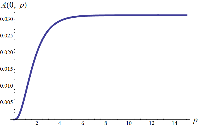
What does this tell us about the quantum dynamics of our model? Recall the definition of the transition amplitude between two quantum states of geometry and , (33). One finds that the main contributions come from those configurations corresponding to classical geometries, namely and large scale factors . The remarkable result is now, that the transition amplitude decreases for small scale factors and has zero support on . This is a statement about the occurrence of singularities in our model in that it tells us that a transition to a singularity is ruled out dynamically.
The transition amplitude now gives us the possibilities for quantum fluctuations from one scale factor to another one. It doesn’t give us the dynamical evolution of our universe. The classical notion of dynamics, i.e. , is encoded in the phase space coordinates. In the same sense as a transition amplitude in QFT does not give us a temporal information of the time evolution of a certain process.
Certainly this result has to be strengthened by future investigations, where it remains to show that one can circumvent the large spin approximation. In fact, one can calculate the traces in (41) in our model explicitly, thanks to the fact that our graph has just one node and thus holds. This way one can in principle avoid the large spin approximation and indeed finds that the amplitude is still peaked on . However, the shape along the direction changes, a problem which probably has to be solved by the use of a different normalization.
IV Discussion
We showed in this paper that within the spinfoam cosmology approach the Daisy graph is sufficient to reproduce the vacuum Friedmann equation for a flat 3-space in the isotropic setting and thus may also be useful for the investigation of anisotropic models. The Daisy graph is perfectly suited to the relaxation of the restriction to isotropic models just by using three different holomorphic labels at each link. This will be our setting in the following paper [47]. Furthermore, we showed how one can reproduce the missing curvature term in the curved model, described by the Dipole graph, without using higher terms in the spin expansion. The right dependence of the real and imaginary part of the holomorphic labels will also be important for the description of the anisotropic model. It has been suggested that the curvature term arises as a ‘higher order’ effect in the prior models. However, this derivation applies even in the flat case, which would contradict the agreement with classical dynamics at large scale factor.
The main result of this work, however, is the statement about the avoidance of singularities in our model. The dynamics of the Daisy graph show zero support for a transition amplitude from a finite scale factor to zero, therefore the singularity itself is not accessed by dynamics. Since the model under consideration does not include matter terms, there can be no direct comparison made with the bouncing models of LQC. It remains to be seen at this stage whether this result is an artefact of approximations made, or is a deeper feature of the full covariant dynamics. A singularity resolution theorem or results analogous to those of [6] would be a strong achievement for the theory. Since the interpretation of a transition amplitude between an in and out state in this model is asymptotic, and we only consider the first order in perturbation theory (in terms of graph expansion, vertex expansion etc) one cannot make any strong claim of singularity avoidance. However, at this order there is a hint of a resolution in the manner of a bounce: Consider a sequence of transitions between scale factors each described with a single transition amplitude. This will be a random walk in the space of scale factors with transition probabilities as described by the distribution in FIG.(3). As the scale factor tends to zero, the probability of moving to a larger scale factor increases, being unity in the limit of zero scale factor. Thus we see that the probability of a collapsing universe continuing to collapse tends to zero, and the probability of expansion tends to one, as we approach the classical singularity, and thus the universe will undergo a bounce. As we have noted, this is a preliminary result, and may not survive extension of the model beyond the simple expansion used here, but nonetheless is encouraging in its similarity to the singularity resolution seen in LQC. Obviously this isn’t the complete picture, as we are moving within points of configuration space at which without giving the detailed dynamics between. This behaviour in which the zero volume state is excluded from solutions hints that singularity resolution may well be a feature of these models, as has recently been argued in [55].
Needless to say, that there are numerous open questions that need to be investigated within the spinfoam cosmology approach, such as the treatment of higher orders in the vertex expansion and of course the inclusion of further spinfoam histories. It is hoped that this will shed some light on the connection with the (quantum reduced) canonical approach as put forward by [17, 56] and also the GFT cosmology in [48]. In the long term perspective the coupling of matter has also high priority if one aims to seriously do quantum cosmology using such models.
Acknowledgments
The authors would like to thank Carlo Rovelli and Francesca Vidotto for useful comments and discussion. DS gratefully acknowledges support from a Templeton Foundation grant. The authors are indebted to the referees whose extensive input has greatly improved this paper.
Appendix A Details of the calculations
In this section we present the calculation of the elements , (35). As explained in section 2.1 the normal vectors and are obtained via a transformation of and the elements and are related to these transformations. We start with and .
| (63) |
| (64) |
We get for and
| (66) |
Analogously one calculates and with the resulting elements
| (67) |
Finally, we have to calculate and but it is clear that is given by
| (68) |
and thus the corresponding elements is
| (69) |
Now we have to connect each two elements with one link. We connect those vectors who are co-linear. Furthermore, we need
| (70) |
The inverse matrices are given by
| (71) |
where we have chosen (71) corresponding to the inverse elements of and resp. The reason is that formula (65) is not valid for a rotation of about the or axis.
We get for the elements
| (72) |
and for and we get analogously
| (73) |
| (74) |
References
- [1] E. Bianchi, C. Rovelli, and F. Vidotto, “Towards spinfoam cosmology,” Phys. Rev. D, vol. 82, Oct 2010. http://link.aps.org/doi/10.1103/PhysRevD.82.084035.
- [2] A. Ashtekar, “Gravity and the quantum,” New Journal of Physics, vol. 7, no. 1, 2005. http://stacks.iop.org/1367-2630/7/i=1/a=198.
- [3] C. Rovelli, “Zakopane lectures on loop gravity,” arXiv:1102.3660v5 [gr-qc], Aug 2011. http://arxiv.org/abs/1102.3660.
- [4] A. Ashtekar, T. Pawlowski, and P. Singh, “Quantum nature of the big bang: Improved dynamics,” Phys. Rev. D, vol. 74, Oct 2006. http://link.aps.org/doi/10.1103/PhysRevD.74.084003.
- [5] M. Bojowald, “Homogeneous loop quantum cosmology,” Classical and Quantum Gravity, vol. 20, no. 13, 2003. http://stacks.iop.org/0264-9381/20/i=13/a=310.
- [6] P. Singh, “Are loop quantum cosmos never singular?,” Classical and Quantum Gravity, vol. 26, no. 12, 2009. http://stacks.iop.org/0264-9381/26/i=12/a=125005.
- [7] P. Singh and F. Vidotto, “Exotic singularities and spatially curved Loop Quantum Cosmology,” Phys.Rev., vol. D83, p. 064027, 2011.
- [8] P. Singh, “Curvature invariants, geodesics and the strength of singularities in Bianchi-I loop quantum cosmology,” Phys.Rev., vol. D85, p. 104011, 2012.
- [9] A. Ashtekar and D. Sloan, “Probability of inflation in loop quantum cosmology,” General Relativity and Gravitation, vol. 43, no. 12, 2011. http://dx.doi.org/10.1007/s10714-011-1246-y.
- [10] I. Agullo, A. Ashtekar, and W. Nelson, “The pre-inflationary dynamics of loop quantum cosmology: confronting quantum gravity with observations,” Classical and Quantum Gravity, vol. 30, no. 8, 2013. http://stacks.iop.org/0264-9381/30/i=8/a=085014.
- [11] J. Engle, R. Pereira, and C. Rovelli, “Loop-quantum-gravity vertex amplitude,” Phys. Rev. Lett., vol. 99, Oct 2007. http://link.aps.org/doi/10.1103/PhysRevLett.99.161301.
- [12] J. Engle, E. Livine, R. Pereira, and C. Rovelli, “LQG vertex with finite Immirzi parameter,” Nuclear Physics B, vol. 799, 2008. http://www.sciencedirect.com/science/article/pii/S0550321308001405.
- [13] R. Pereira, “Lorentzian loop quantum gravity vertex amplitude,” Classical and Quantum Gravity, vol. 25, no. 8, 2008. http://stacks.iop.org/0264-9381/25/i=8/a=085013.
- [14] W. Kaminski, M. Kisielowski, and J. Lewandowskii, “Spin-foams for all loop quantum gravity,” Classical and Quantum Gravity, vol. 27, no. 9, 2010. http://stacks.iop.org/0264-9381/27/i=9/a=095006.
- [15] E. Bianchi, T. Krajewski, C. Rovelli, and F. Vidotto, “Cosmological constant in spinfoam cosmology,” Phys. Rev. D, vol. 83, May 2011. http://link.aps.org/doi/10.1103/PhysRevD.83.104015.
- [16] A. Baratin, C. Flori, and T. Thiemann, “The holst spin foam model via cubulations,” New Journal of Physics, vol. 14, Oct 2012. http://stacks.iop.org/1367-2630/14/i=10/a=103054.
- [17] E. Alesci and F. Cianfrani, “Quantum - Reduced Loop Gravity: Cosmology,” arXiv:1301.2245 [gr-qc], Jan 2013. http://arxiv.org/abs/1301.2245.
- [18] A. Ashtekar and E. Wilson-Ewing, “Loop quantum cosmology of Bianchi type I models,” Phys. Rev. D, vol. 79, Apr 2009. http://link.aps.org/doi/10.1103/PhysRevD.79.083535.
- [19] A. Ashtekar and E. Wilson-Ewing, “Loop quantum cosmology of Bianchi type II models,” Phys. Rev. D, vol. 80, Dec 2009. http://link.aps.org/doi/10.1103/PhysRevD.80.123532.
- [20] E. Wilson-Ewing, “Loop quantum cosmology of Bianchi type IX models,” Phys. Rev. D, vol. 82, Aug 2010. http://link.aps.org/doi/10.1103/PhysRevD.82.043508.
- [21] A. Corichi and E. Montoya, “Effective dynamics in Bianchi type II loop quantum cosmology,” Phys. Rev. D, vol. 85, May 2012. http://link.aps.org/doi/10.1103/PhysRevD.85.104052.
- [22] D.-W. Chiou and K. Vandersloot, “The Behavior of non-linear anisotropies in bouncing Bianchi I models of loop quantum cosmology,” Phys.Rev., vol. D76, p. 084015, 2007.
- [23] T. Cailleteau, P. Singh, and K. Vandersloot, “Non-singular Ekpyrotic/Cyclic model in Loop Quantum Cosmology,” Phys.Rev., vol. D80, p. 124013, 2009.
- [24] D.-W. Chiou, “Loop Quantum Cosmology in Bianchi Type I Models: Analytical Investigation,” Phys.Rev., vol. D75, p. 024029, 2007.
- [25] R. Maartens and K. Vandersloot, “Magnetic Bianchi I Universe in Loop Quantum Cosmology,” arXiv:0812.1889 [gr-qc], Dec 2008. http://arxiv.org/abs/0812.1889.
- [26] B. Gupt and P. Singh, “Contrasting features of anisotropic loop quantum cosmologies: The Role of spatial curvature,” Phys.Rev., vol. D85, p. 044011, 2012.
- [27] A. Corichi and E. Montoya, “Qualitative effective dynamics in Bianchi II loop quantum cosmology,” AIP Conference Proceedings, vol. 1473, no. 1, 2012. http://link.aip.org/link/?APC/1473/113/1.
- [28] B. Gupt and P. Singh, “Quantum gravitational Kasner transitions in Bianchi-I spacetime,” Phys.Rev., vol. D86, p. 024034, 2012.
- [29] A. Corichi, A. Karami, and E. Montoya, “Loop Quantum Cosmology: Anisotropy and singularity resolution,” arXiv:1210.7248v2 [gr-qc], Dec 2012. http://arxiv.org/abs/1210.7248.
- [30] C. Rovelli, Quantum gravity. Cambridge monographs on mathematical physics, Cambridge Univ. Press, 2010.
- [31] E. Bianchi, E. Magliaro, and C. Perini, “Spinfoams in the holomorphic representation,” Phys. Rev. D, vol. 82, Dec 2010. http://link.aps.org/doi/10.1103/PhysRevD.82.124031.
- [32] R. Oeckl, “A “general boundary” formulation for quantum mechanics and quantum gravity,” Physics Letters B, vol. 575, no. 3–4, pp. 318 – 324, 2003. http://www.sciencedirect.com/science/article/pii/S0370269303013066.
- [33] R. Oeckl, “Probabilites in the general boundary formulation,” Journal of Physics: Conference Series, vol. 67, no. 1, p. 012049, 2007. http://stacks.iop.org/1742-6596/67/i=1/a=012049.
- [34] R. Oeckl, “General boundary quantum field theory: Foundations and probability interpretation,” Advances in Theoretical and Mathematical Physics, vol. 12, no. 2, 2008. http://intlpress.com/site/pub/pages/journals/items/atmp/content/vols/0012/0002/00024708/index.html.
- [35] E. R. Livine and S. Speziale, “New spinfoam vertex for quantum gravity,” Phys. Rev. D, vol. 76, Oct 2007. http://link.aps.org/doi/10.1103/PhysRevD.76.084028.
- [36] E. Bianchi, E. Magliaro, and C. Perini, “Coherent spin-networks,” Phys. Rev. D, vol. 82, Jul 2010. http://link.aps.org/doi/10.1103/PhysRevD.82.024012.
- [37] D. Oriti, R. Pereira, and L. Sindon, “Coherent states in quantum gravity: a construction based on the flux representation of LQG,” arXiv:1110.5885 [gr-qc], Oct 2011. http://arxiv.org/abs/1110.5885.
- [38] D. Oriti, R. Pereira, and L. Sindon, “Coherent states for quantum gravity: towards collective variables,” arXiv:1202.0526 [gr-qc], Feb 2012. http://arxiv.org/abs/1202.0526.
- [39] A. Pittelli and L. Sindoni, “New coherent states and modified heat equations,” arXiv:1301.3113 [gr-qc], Jan 2013. http://arxiv.org/abs/1301.3113.
- [40] M. Bojowald, “Loop quantum cosmology: I. kinematics,” Classical and Quantum Gravity, vol. 17, no. 6, 2000. http://stacks.iop.org/0264-9381/17/i=6/a=312.
- [41] M. Bojowald, “Isotropic loop quantum cosmology,” Classical and Quantum Gravity, vol. 19, no. 10, 2002. http://stacks.iop.org/0264-9381/19/i=10/a=313.
- [42] M. Bojowald, G. Date, and K. Vandersloot, “Homogeneous loop quantum cosmology: the role of the spin connection,” Classical and Quantum Gravity, vol. 21, no. 4, 2004. http://stacks.iop.org/0264-9381/21/i=4/a=034.
- [43] M. V. Battisti, A. Marcianò, and C. Rovelli, “Triangulated loop quantum cosmology: Bianchi IX universe and inhomogeneous perturbations,” Phys. Rev. D, vol. 81, Mar 2010. http://link.aps.org/doi/10.1103/PhysRevD.81.064019.
- [44] T. Thiemann and O. Winkler, “Gauge field theory coherent states (GCS): II. Peakedness properties,” Classical and Quantum Gravity, vol. 18, no. 14, 2001. http://stacks.iop.org/0264-9381/18/i=14/a=301.
- [45] M. Bojowald, Quantum Cosmology: A Fundamental Description of the Universe. Springer, (Lecture Notes in Physics), 2011.
- [46] T. Thiemann, Modern Canonical Quantum General Relativity. Cambridge monographs on mathematical physics, Cambridge University Press, 1st ed., 2008.
- [47] J. Rennert and D. Sloan, “Anisotropic Spinfoam Cosmology,” arXiv:1308.0687 [gr-qc], Aug 2013. http://arxiv.org/abs/1308.0687.
- [48] S. Gielen, D. Oriti, and L. Sindoni, “Cosmology from group field theory formalism for quantum gravity,” Phys. Rev. Lett., vol. 111, Jul 2013. http://link.aps.org/doi/10.1103/PhysRevLett.111.031301.
- [49] C. Rovelli, “Discretizing parametrized systems: the magic of Ditt-invariance,” arXiv:1107.2310 [hep-lat], Aug 2011. http://arxiv.org/abs/1107.2310.
- [50] C. Rovelli, “On the structure of a background independent quantum theory: Hamilton function, transition amplitudes, classical limit and continuous limit,” arXiv:1108.0832 [gr-qc], Aug 2011. http://arxiv.org/abs/1108.0832.
- [51] F. Hellmann, “Expansions in spin foam cosmology,” Phys. Rev. D, vol. 84, Nov 2011. http://link.aps.org/doi/10.1103/PhysRevD.84.103516.
- [52] M. Kisielowski, J. Lewandowski, and J. Puchta, “One vertex spin-foams with the dipole cosmology boundary,” arXiv:1203.1530v1 [gr-qc], Mar 2012. http://arxiv.org/abs/1203.1530.
- [53] J. Engle and R. Pereira, “Regularization and finiteness of the lorentzian loop quantum gravity vertices,” Phys. Rev. D, vol. 79, Apr 2009. http://link.aps.org/doi/10.1103/PhysRevD.79.084034.
- [54] D. M. Brink and G. R. Satchler, Angular Momentum. Oxford University Press, USA, 3 ed., Mar 1994.
- [55] C. Rovelli and F. Vidotto, “Maximal acceleration in covariant loop gravity and singularity resolution,” arXiv:1307.3228 [gr-qc], Jul 2013. http://arxiv.org/abs/1307.3228.
- [56] E. Alesci and F. Cianfrani, “A new perspective on cosmology in Loop Quantum Gravity,” arXiv:1210.4504 [gr-qc], Oct 2012. http://arxiv.org/abs/1210.4504.
- [57] M. Carmeli, Group Theory and General Relativity - Representations of the Lorentz Group and Their Applications to the Gravitational Field. McGraw-Hill Inc.,US, Aug 1977.
- [58] R. U. Sexl and H. K. Urbantke, Relativity, Groups, Particles: Special Relativity - Relativistic Symmetry in Field and Particle Physics. Springer, 1 ed., Nov 2000.