Fermi surface in KFe2As2 determined via de Haas-van Alphen oscillation measurements
Abstract
We have completely determined the Fermi surface in KFe2As2 via de Haas-van Alphen (dHvA) measurements. Fundamental frequencies , , , and are observed in KFe2As2. The first one is attributed to a hole cylinder near the X point of the Brillouin zone, while the others to hole cylinders at the point. We also observe magnetic breakdown frequencies between and and suggest a plausible explanation for them. The experimental frequencies show deviations from frequencies predicted by band structure calculations. Large effective masses up to 19 for have been found, being the free electron mass. The carrier number and Sommerfeld coefficient of the specific heat are estimated to be 1.01 – 1.03 holes per formula unit and 82 – 94 mJmol-1K-2, respectively, which are consistent with the chemical stoichiometry and a direct measure of 93 mJmol-1K-2 [H. Fukazawa et al., J. Phys. Soc. Jpn. 80SA, SA118 (2011)]. The Sommerfeld coefficient is about 9 times enhanced over a band value, suggesting the importance of low-energy spin and/or orbital fluctuations, and places KFe2As2 among strongly correlated metals. We have also performed dHvA measurements on Ba0.07K0.93Fe2As2 and have observed the and frequencies.
pacs
71.18.+y, 74.70.Xa, 71.27.+aI Introduction
Since the discovery of superconductivity at = 26 K in LaFeAs(O, F) by Kamihara et al.,[1] iron-pnicitde/selenide high- superconductivity has been a center of activity in the condensed matter physics community.[[Forreviews, see]Ishida09JPSJ_review, *Johnston10AdvPhys] Many different materials have been synthesized and has quickly been raised up to 55 K.[4, 5, 6, 7] The superconducting pairing mechanism is still under debate;[8] spin fluctuations on the one hand and orbital fluctuations on the other hand. Basically, the former approach predicts an gap that changes sign between electron and hole Fermi surface (FS) pockets,[9, 10] while the latter predicts an gap without sign change.[11]
Ba1-xKxFe2As2 (Ref. 12) is one of the most studied systems. High-quality single crystals can be grown by flux method. The parent material BaFe2As2 orders antiferromagnetically below the Néel temperature = 140 K (Ref. 13) and is a moderately correlated metal with mass enhancements of 2 – 3 in the ground state, and being the effective and the band mass, respectively.[14, 15] As K is substituted for Ba, the antiferromagnetism is suppressed and disappears at , and superconductivity appears.[16] reaches 38 K at optimal doping .[12] does not disappear till = 1;[17, 16, 18] KFe2As2 is a superconductor with = 3.4 K.[19]
Intriguingly, the superconducting gap structure seems to change with in Ba1-xKxFe2As2. Near the optimal doping, a fully gapped -wave superconductivity has been indicated by penetration depth,[20] specific heat,[21, 22] thermal conductivity,[23] and NMR measurements.[24] On the other hand, a nodal gap structure in KFe2As2 has been suggested by NMR, specific heat,[25] penetration depth[26] and thermal conductivity measurements.[[][.However, noteRef.~\cite[citep]{\@@bibref{Number}{Terashima10PRL_comment}{}{}}.]Dong10PRL, 28, 29] A laser angle-resolved photoemission spectroscopy (laser ARPES) and an NMR study as a function of the composition have found a drastic change in the gap structure around = 0.6.[30, 31] Although it has been under debate whether the superconducting state is an -wave or -wave one,[29] the octet-line nodes of the gap recently observed in another laser ARPES study[32] are compatible with an -wave state with accidental nodes. Theoretical studies based on the spin-fluctuations approach suggest a variety of gap structures with - or -wave symmetries depending on band and interaction parameters.[33, 34, 35]
In this context, precise determination of the electronic structure near the Fermi level in KFe2As2 is highly desirable. Previously, we reported de Haas-van Alphen (dHvA) measurements on KFe2As2 in a letter.[36] We observed one small FS cylinder and two relatively large ones. With the aid of band structure calculations, they were assigned to a hole cylinder near the X point of the Brillouin zone (BZ) and hole cylinders at the point, respectively. We thought that the largest hole cylinder at expected from band structure calculations was not observed. Recently, we have observed dHvA oscillations in Ba0.07K0.93Fe2As2. Interestingly, the largest FS cylinder is clearly observed. Motivated by this observation, we have reexamined dHvA oscillations in KFe2As2, and have noticed that the largest cylinder is also observed in KFe2As2. Thus we have completely determined the Fermi surface in KFe2As2 via dHvA measurements. The mass enhancement amounts to 9, which is much larger than the overall band-width renormalization of 2 estimated in an early ARPES study[37] and indicates the importance of low-energy spin and/or orbital fluctuations. In addition, we explain magnetic breakdown frequencies observed between the and orbits assuming eight magnetic breakdown junctions, the positions of which resemble those of the octet-line nodes.
II Experiments, Lifshitz-Kosevich formula, and Yamaji model
High-quality single crystals of KFe2As2 and Ba0.07K0.93Fe2As2 were grown by a self flux method as described in Ref. 19. Large residual resistivity ratios of more than 450 and of 70 were observed for KFe2As2 and K0.93Ba0.07Fe2As2, respectively.[19] In the case of KFe2As2, nine different crystals were measured and gave consistent results. We describe results obtained for the most thoroughly measured sample.
The dHvA measurements were performed in a dilution refrigerator and superconducting magnet by using the field modulation technique.[38] The modulation frequency and amplitude were mostly = 67.1 Hz and = 10.4 mT, respectively, and the detection was made at the second harmonic (2). A sample was placed in a balanced pick-up coil with its axis parallel to the coil axis. The field direction measured from the axis is denoted by , and if necessary a subscript is attached to indicate the field-rotation plane. The same setup was used to measure ac magnetic susceptibility.
The dHvA magnetization oscillation due to an extremal cyclotron orbit normal to enclosing the -space area is given by[38]
| (1) |
where
| (2) | |||
| (3) | |||
| (4) | |||
| (5) |
Here , being the free electron mass. The effective mass is enhanced over the band mass by electron-phonon and electron-electron interactions. The frequency is given by , and is the phase. Not only the fundamental frequency but also its harmonics () appear in . is the curvature factor: , where is the wave number along . is the temperature reduction factor, where is a constant (14.69 T/K). The Dingle factor describes the influence of disorder/impurity scattering, being the Dingle temperature. We can determine and by fitting and to - and -dependences of experimental oscillation amplitudes at constant and , respectively. The spin reduction factor is due to the interference between oscillations from up- and down-spin electrons, and the spin-splitting parameter may be expressed as with an effective factor .
With the present setup and second-harmonic detection, amplitudes of oscillations in the detected voltage, , are related to as
| (6) |
where is the second-order Bessel function, and . We distinguish the two amplitudes and when necessary.
In the case of a purely two-dimensional (2D) electronic structure, the FS would be a straight cylinder showing a single dHvA frequency , and would be constant irrespective of the field direction . With a quadratic in-plane dispersion, would also be constant; i.e., , being the effective mass for . Given the crystal structure of KFe2As2, each FS cylinder would contribute
| (7) |
to the Sommerfeld coefficient of the specific heat, where . Note that the contribution does not depends on the size of the FS cylinder. 11 1 For a 2D system, the number of states is given by , where is the FS cross section normal to the axis and is the thickness of the Brillouin zone along the axis. Since , the density of states is proportional to but does not depend on the FS size.
In reality, there is a -axis dispersion of the electronic band energy, which leads to corrugation of the cylindrical FS and produces at least two dHvA frequencies corresponding to the maximal and minimal FS cross sections. Yamaji considered the simplest case where the -axis dispersion takes a form of , where is the interlayer distance and equals in KFe2As2, and derived the angular dependence of the two frequencies:[40]
| (8) |
where and are the average of and the difference between the two frequencies at = 0, respectively, is the zeroth-order Bessel function, and is the in-plane Fermi wave number. At magic angles where (: integer), the two frequencies coincide, resulting in single-frequency dHvA oscillations with an enhanced amplitude. It is also known that the interlayer magnetoresistance at a constant field shows maxima at these field angles as a function of the field direction when the field is tilted from the axis. This phenomenon is called angle dependent magnetoresistance oscillation (AMRO) and is used to determine the FS in quasi-2D metals. The phase is 1/4 for the above simplest dispersion but actually varies depending on details of the -axis dispersion.
III Results
III.1 Upper critical field

Figure 1(a) shows pick-up coil signals detected at the modulation frequency as a function of magnetic field for KFe2As2.22 2 Pick-up coil signals detected at the modulation frequency are proportional to ac magnetic susceptibilities for . In the case of , the coil axis is perpendicular to , since the coil and sample are rotated together with the axis kept parallel to the coil axis. If the alignment of the sample and coil axis is perfect, no signal will be detected. However, there is small misalignment, which produces small signal proportional to the component of ac magnetization along the coil axis for . From these data, we estimate that the upper critical field in this sample is 1.7 T at = 0.17 K for and 4.9 T at = 0.18 K for . These values are slightly larger than those previously determined for a lower-quality sample.[42] We note that the -plane critical field, which is consistent with Ref. 43, is much lower than the orbital critical field (7 T) estimated from the initial slope of at in samples of similar quality to the present one,[44, 45] confirming the existence of strong spin paramagnetic effects.[42]
III.2 dHvA oscillations
Figure 2 shows examples of dHvA oscillations. For KFe2As2, the frequency of prominent oscillations for is about 2.4 kT both at low fields and at high fields, though higher frequencies are also noticeable at high fields. The oscillations continue down to below 3 T.[28] For Ba0.07K0.93Fe2As2, the frequency of prominent oscillations is about 6.7 kT.

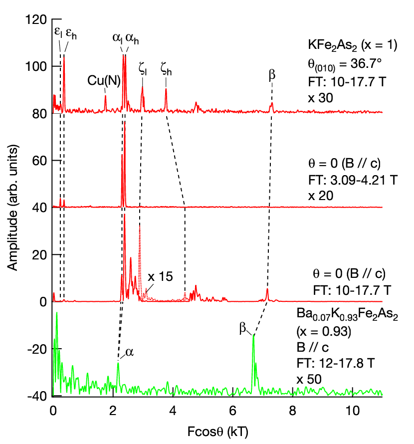


Figure 3 shows representative Fourier transforms of dHvA oscillations for the two compounds. Fundamental frequencies, , , , and , are indicated. The identification of these fundamentals is explained below. We note that the and frequencies in Ba0.07K0.93Fe2As2 are about 93% of those in KFe2As2, which is consistent with the carrier number expected from the composition = 0.93. Figures 4 and 5 show details of angular variation of dHvA oscillations in KFe2As2 for fields in the (010) and the (10) plane, respectively. The angle dependences of the observed frequencies are shown in Fig. 6(b). Figure 7 shows angular variation of dHvA oscillations in Ba0.07K0.93Fe2As2 for fields in the (010). In the case of Ba0.07K0.93Fe2As2, three frequencies arising from materials of the pick-up coil assembly have comparable amplitudes to the frequencies from the sample: i.e., copper neck frequency, its second harmonic, and an unknown frequency, which might be due to tin from solder used for wiring. However, they have detectable amplitudes only for .33 3 This is related to the imbalance of the pick-up coil. The pick-up coil is composed of coaxially wound inner and outer coils. The two coils are balanced without a sample at = 0 so that the emf’s induced in the two coils cancel each other out. The balance however degrades as increases. We show Fourier transforms of pick-up coil signals without a sample for some field directions for comparison (dotted spectra), which clearly indicate that the and frequencies arise from the sample, not from the coil assembly.
Figures 8 and 9 exemplify determination of effective masses for KFe2As2 and Ba0.07K0.93Fe2As2, respectively. The determined masses are tabulated in Tables I and II. Heavy masses up to 19 for are observed for KFe2As2. The masses in Ba0.07K0.93Fe2As2 are nearly the same as the corresponding masses in KFe2As2.


| Field direction | Branch | (kT) | (K) | |
|---|---|---|---|---|
| 0.24 | 6.0(4) | 0.14(2) | ||
| 0.36 | 7.2(2) | 0.18(1) | ||
| 2.30 | 6.0(2) | 0.19(2) | ||
| 2.39 | 6.5(2) | 0.18(2) | ||
| 2.89 | 8.5(2) | 0.1 | ||
| 4.40 | 18(2) | |||
| 7.16 | 19(2) | |||
| 0.30 | 7.4(7) | |||
| 0.45 | 8.4(2) | |||
| 2.91 | 7.4(2) | |||
| 11 1 Extra splitting observed. | 2.98 | 7.8(2) | ||
| 11 1 Extra splitting observed. | 3.02 | 7.4(2) | ||
| 3.72 | 11.1(4) | |||
| 4.70 | 12.5(7) | |||
| 9.12 | 20(3) | |||
| 0.32 | 7.7(7) | |||
| 0.47 | 9(2) | |||
| 3.05 | 6.9(3) | |||
| 3.13 | 7.7(2) | |||
| 11 1 Extra splitting observed. | 3.95 | 11(1) | ||
| 11 1 Extra splitting observed. | 3.99 | 13(1) | ||
| 4.75 | 11(1) | |||
| unobserved |
| Field direction | Branch | (kT) | |
|---|---|---|---|
| 2.17 | 4(1) | ||
| 6.69 | 18(2) | ||
| 6.77 | 16(3) |
III.3 Fundamental frequencies


A pair of frequencies and near = 0.3 kT in KFe2As2 [Figs. 4, 5, and 6(b)] can be assigned to the minimum and maximum orbits on a corrugated FS cylinder. Their angular variation is consistent with the Yamaji model as indicated in the figures.
A complex region between = 2 and 3 kT for in KFe2As2 is shown in Fig. 10(a) in an expanded scale. We identify three frequencies , , and as fundamentals. All the other frequencies can be indexed with a formula (: integer), where . Their amplitudes are quickly suppressed as the field is decreased [compare the three spectra for three different field windows in Fig. 10(a)]. To be more quantitative, Fig. 11 shows the field dependence of amplitudes of various frequencies for in KFe2As2 in the form of Dingle plot. The Dingle temperatures for fundamental frequencies estimated from the plots are shown in Table I. (We can also estimate mean free paths of about 100 and 300 nm for and , respectively.) It is clear that the non-fundamental frequencies are suppressed with decreasing field more quickly than the fundamental frequencies. These observations strongly suggest that the frequencies other than , , and are due to magnetic breakdown orbits between and . We observed essentially the same spectra and field dependence in other samples.
Figure 12 shows schematically the and orbits deduced from recent ARPES measurements.[48, 49, 50] There are eight possible magnetic breakdown junctions as indicated. If area A1 is approximately twice area A2 and hence and , the observed magnetic breakdown frequencies can be explained: frequency = 1 corresponds to , = 2 to and , = 3 to and , and so on. It is interesting that the positions of the inferred magnetic breakdown junctions remind us of those of the octet-line nodes in the superconducting gap observed in a laser-ARPES study.[32]
Figure 10(b) shows a frequency region near the second harmonic of in an expanded scale. Many frequencies are observed above 2, and they (except 2) can be indexed with (: integer). However, a small peak at = 4.40 kT can not be indexed and we identify it as the counterpart of , namely .
Detailed angular dependence of in KFe2As2 is shown in the right panels of Figs. 4 and 5. As the field is tilted from the axis, the two peaks gradually approach and roughly merge when is or when is slightly larger than 40∘. The amplitudes at these magic angles are enhanced when compared to those at neighboring angles. These observations are basically consistent with the Yamaji model (dashed lines). Slight deviations of the peak positions from the model and extra splitting of the frequencies, which is especially noticeable at high angles , can be explained by small error in and small distribution of the -axis orientation in the sample. The shading in the figures illustrates how the frequencies spread if there is a error or distribution of the -axis orientation. The magic angles also deviate from the Yamaji model and exhibit in-plane anisotropy; i.e, the magic angle in the (010) plane is slightly larger than that in the (10) plane. This indicates in-plane anisotropy of and/or more complex -axis dispersion than the Yamaji model. The observed magic angles and their anisotropy are consistent with those observed in AMRO measurements.[51]
The angular dependence of [Figs. 4, 5, and 6(b)] indicates that the sheet is the most three-dimsnsional sheet of the Fermi surface. The maximum frequency exhibits much more variation in than the minimum frequency . This indicates that, while the cylinder is close to a straight one around the minimum cross section, it swells out locally around the maximum cross section. For , the effective mass of is considerably larger than that of (Table I). As the field is tilted, the masses of the two frequencies become nearly the same (see the masses determined at = 36.7∘ and = 40.5∘ in Table I). This also indicates that the deformation of the cylinder is local near the maximum cross section.
We now turn to the frequency in KFe2As2. In the previous paper,[36] we identified this frequency with the third harmonic of because it satisfies the relations and within experimental accuracy (Table I). However, we have recently observed the frequency very clearly in Ba0.07K0.93Fe2As2 (Figs. 3 and 7), where is unmistakably different from . The effective mass of in Ba0.07K0.93Fe2As2 is close to that in KFe2As2 (Tables I and II). These findings have motivated us to reexamine the frequency in KFe2As2, and we have reached the conclusion that it is a fundamental frequency as explained below.
First of all, the amplitudes of the frequency appear too big for a third harmonic (Figs. 4 and 5). According to the Lifshitz-Kosevich formula, amplitudes of harmonics basically decrease exponentially with the harmonic number . Because of the spin factor , which oscillates with , the third harmonic can accidentally be comparable to or even larger than the second harmonic for some field directions. 44 4 Because varies as , in Eq. (5) varies with . However, the frequency in KFe2As2 has a comparable amplitude to the second harmonic of for a wide range of field directions, which seems difficult to explain if it is the third harmonic.
To be more quantitative, we analyze the amplitudes of , its second harmonic, and for , using Eqs. (1)-(6). Since the effective mass and the Dingle temperature for the frequency have been determined from the temperature and field dependences of the amplitude (Table I), we can determine the spin-splitting parameter from the amplitudes of the fundamental and second harmonic (Fig. 13): or (: integer). Using these values of , we can estimate the amplitude of the third harmonic. In either case, the estimated amplitude is significantly smaller than the observed amplitude of the frequency. It thus follows that, although there is some contribution from the third harmonic of , the observed amplitude of at = 0 is mostly due to the fundamental frequency .
There is a further evidence for the fundamental : the frequency of deviates from that of the third harmonic of at high angles as shown in Fig. 14. We therefore conclude that the frequency is a fundamental frequency.
It is unclear at present whether the observed frequency is a maximum or a minimum frequency. A small peak at = 7.44 kT at = 0 might perhaps be the counterpart (Figs. 4 and 5).
The experimentally determined Fermi surface in KFe2As2 is schematically shown in Fig. 15(c).
Lastly, we briefly discuss Ba0.07K0.93Fe2As2. The minimum and maximum frequencies of are not resolved in Fig. 7. This is probably because the oscillation is so weak that the quality of the signal is insufficient to resolve the two finely-spaced frequencies. On the other hand, the frequency splits at = 0 (Fig. 7 or Fig. 9). If the two frequencies are the minimum and maximum frequencies, it follows that the cylinder is strongly two dimensional ( = 1.2%). The and frequencies were not observed in Ba0.07K0.93Fe2As2. This is probably because they are too weak.
The and frequencies in Ba0.07K0.93Fe2As2 are both approximately 93% of those in KFe2As2 and are consistent with the composition = 0.93 within experimental error. This is compatible with a rigid band picture. Within an effective mass approximation, . Hence, a dHvA frequency shift due to a shift in the Fermi energy satisfies a relation . Therefore, if two bands have the same , for a energy shift is the same for both bands. Assuming the same mass renormalization for both bands, . Since = 0.38 kT for both and orbits in KFe2As2, should be the same as observed.


IV Comparison to band structure calculations

The electronic band structure of KFe2As2 was calculated within the local density approximation (LDA) by using a full-potential linearized augmented plane-wave (FLAPW) method.[36] We used the program codes TSPACE[53] and KANSAI-06. The experimental crystal structure [54] including the atomic position of As was used for the calculation. The calculated Fermi surface is shown in Fig. 15, and the electronic band structure and density of states (DOS) are shown in Fig. 16. The spin-orbit interaction has been included in these calculations. The DOS at the Fermi level () is 58.4 states/(Ry f.u.), which corresponds to the Sommerfeld coefficient of = 10.1 mJ/K2mol. Note that a direct specific-heat measurement gives = 93 mJ/K2mol,[55] indicating a large mass enhancement of = 9 due to electronic correlations. As can be seen from the DOS plot [Fig. 16(c)], the states near are mostly derived from the Fe 3 orbitals. Four bands 31–34 cross [Fig. 16(b)], and the FS consists of three concentric hole cylinders at the point of the BZ (bands-32, 33, and 34), small hole cylinders near the zone boundary (band-34), and a small hole pocket at Z (band-31) [Fig. 15(a)]. Note that the band-34 small hole cylinders are situated inside the Brillouin zone, not on the border, and hence there are four of them per Brillouin zone [Fig. 15(b)]. A previous calculation,[56] where was relaxed by energy minimization, predicted an electron cylinder at X instead of the hole cylinders near X. However, ARPES measurements so far have found no electron cylinder in KFe2As2 and are qualitatively consistent with the presently calculated FS.[37, 48, 50]
For the observed dHvA frequencies, it is clear that the , , and cylinders correspond to the three hole cylinders at and the cylinder to the small hole cylinder near X (Fig. 15). However, the quantitative agreement is poor as can be seen in Fig. 6, where the calculated and experimental frequencies are shown. Calculated band masses ranging from 0.3 to 2.9 for are much smaller than the observed effective masses (Table I), again suggesting the strong correlations.
To see if the agreement can be improved, we have adjusted the band energies so that the smallest band-32 cylinder matches the cylinder and that the largest band-34 cylinder matches the cylinder. The energy of band-33 was adjusted to keep the total carrier number. The small band-31 pocket was neglected. The resultant frequencies are shown in Fig. 6(c). The large undulation of the cylinder can not be reproduced by the calculation. 55 5 The adjusted calculation gives a Sommerfeld coefficient of 33.1 mJ/K2mol. However, the validity of this estimate is questioned because the adjustment can not reproduce the observed FS.
V Discussion
The failure of LDA calculations in KFe2As2 contrasts sharply with the case of BaFe2As2, where LDA calculations give basically correct description of the Fermi surface (despite the overestimation of the antiferromagnetic moment).[15] It seems that LDA band structure calculations fail to predict crystal field splitting of the Fe levels in KFe2As2. In the calculated band structure, one band is situated immediately above at the point and two nearly degenerate bands are situated above it [Fig. 16(b)]. The former band is of character. The latter two bands are of / character and would be truly degenerate if spin-orbit coupling were absent. However, experimental observation is that there are two similarly sized relatively small cylinders ( and ) and one relatively large cylinder () at the point. This strongly suggests that the / bands are actually lower than the band and produce the and cylinders. In fact, these orbital characters have been confirmed by recent ARPES measurements.[32, 50]
Dynamical mean field theory (DMFT) studies have shown that the crystal field splitting of the Fe levels may be modified if electronic correlations are treated beyond the LDA.[58, 59] A recent DMFT calculation[60] suggests that the order of the and / bands at the point in KFe2As2 are inverted by electronic correlations. However, it should also be noted that the crystal field splitting is affected by hybridization between the Fe 3 and As 4 as well as Fe 4 states. Given the well known problem of band structure calculations in iron pnictides that structural optimization for paramagnetic states can not predict the correct position of As, this hybridization may not be calculated very accurately within the LDA, which would affect the crystal field splitting of the Fe 3 levels. This point deserves further studies.
| dHvA (present work) | ARPES | AMRO | |||||
| Ref. 37 | Ref. 48 | Ref. 51 | |||||
| FS | (%BZ) | (mJ mol-1K-2) | (%BZ) | (mJ mol-1K-2) | (%BZ) | (%BZ) | (%BZ) |
| 11 1 There are four cylinders in the BZ. | 1.1 4 | 9.6 4 | 1.1 4 | 9.1 4 | 2.5 | 2.1 4 | |
| 8.4 | 9.1 | 8.5 | 8.7 | 7 | 10.1 | 12 | |
| 13.0 | 19.2 | 12.1 | 13.7 | 11.8 | 17 | ||
| 25.6 | 27.6 | 25.5 | 23.2 | 22 2 | 28.5 | ||
| total | 51.4 | 94 | 50.5 | 82 | 53.5 | 58.8 | |
We can estimate the Fermi surface volume and Sommerfeld coefficient of the specific heat from the determined FS within a 2D approximation (Table III). We have used two data sets, one at =0 and the other at = 36.7∘, separately for the estimation, and have obtained consistent results.
The estimated FS volume corresponds to the carrier number of 1.01 – 1.03 holes/f.u., which is consistent with the stoichiometry of KFe2As2 within experimental error. We also compare the sizes of the observed FS cylinders with those obtained by ARPES[37, 48] and AMRO[51] measurements in Table III. The more recent ARPES data (Ref. 48) are in reasonable agreement with the present data. Usually AMRO measurements give quantitative estimates of FS sizes, but in the present case the agreement with the present data is limited, which is ascribed to the fact that only a small number of broad AMRO peaks were observed.[51]
The Sommerfeld coefficient is estimated to be 82 – 94 mJmol-1K-2, which is consistent with the direct measure of = 93 mJmol-1K-2 (Ref. 55 and also Ref. 61) and also with an estimate of 84 mJmol-1K-2 in a recent ARPES study,[50] where effective masses have been determined from band dispersions near the Fermi level. These confirm a mass enhancement of about 9 in KFe2As2. Therefore, the electronic correlations are much stronger in KFe2As2 than in BaFe2As2, where mass enhancements are 2 – 3.
It is interesting to recall here that overall band-width renormalization factors estimated in early ARPES studies do not vary significantly with the chemical composition in the Ba1-xKxFe2As2 system: 1.5 in BaFe2As2,[62] 2.7 in Ba0.6K0.4Fe2As2,[62] and 2 in KFe2As2.[37] On the theoretical side, a study based on the fluctuation exchange (FLEX) approximation has predicted a significant growth in the mass enhancement from BaFe2As2 to KFe2As2,[63] while the DMFT study of Ref. 60 suggests similar mass enhancements for both BaFe2As2 and KFe2As2. These seemingly contradicting results can be reconciled if one notices the existence of two distinct mechanisms contributing to the mass enhancement as previously pointed out.[64] One is narrowing of overall band widths, which can be measured as band-width renormalization factors in ARPES measurements and seems to be dealt with a DMFT fairly well. The other is flattening of bands near the Fermi level, which arises from interaction with low-energy bosonic excitations. The large discrepancy between the dHvA mass enhancement and the ARPES band-width renormalization factor in KFe2As2 indicates that this latter effect, which involves spin and orbital fluctuations, grows from BaFe2As2 to KFe2As2 as suggested by the FLEX study.[63] The existence of strong spin fluctuations in KFe2As2 has been evidenced by inelastic neutron scattering[65] and NMR measurements.[66, 31]
VI Summary
We have performed dHvA measurements on KFe2As2 and Ba0.07K0.93Fe2As2. For KFe2As2, we have identified frequencies , , , and as fundamentals. The rest of observed frequencies are attributed to harmonics and magnetic breakdown orbits between and . The positions of the inferred magnetic breakdown junctions between and resemble those of the octet-line nodes of the superconducting energy gap.[32] With the aid of LDA band structure calculations, we have assigned the frequency to a hole FS cylinder near the X point and the , , and frequencies to three concentric hole cylinders at the point. On a quantitative level, however, the agreement between the observed and calculated frequencies is poor. This can be attributed to the fact that the crystal field splitting of the Fe 3 levels are not correctly calculated. Effective masses are large, up to 19 for . From the dHvA data, we estimate the carrier concentration and Sommerfeld coefficient to be 1.01 – 1.03 holes/f.u. and 82 – 94 mJmol-1K-2, respectively. They are consistent with the chemical stoichiometry and a direct measure of 93 mJmol-1K-2,[55] respectively, establishing that the determined FS is complete. The large Sommerfeld coefficient, which is about 9 times larger than a band value, indicates that KFe2As2 is a strongly correlated metal. The discrepancy between the mass enhancement of 9 and the ARPES overall band-width renormalization of 2 (Ref. 37) suggests the importance of low-energy spin and/or orbital fluctuations. For Ba0.07K0.93Fe2As2, we have observed the and frequencies. The frequency change between the two compounds can be understood within a rigid-band model.
Acknowledgements.
TT thanks T. Yoshida for valuable discussions; especially, he pointed out possible relation between the magnetic breakdown junctions and octet-line nodes. This work was supported by Grants-in-Aid for Scientific Research (Nos. 21540351, 22540380, and 22684016) from MEXT and JSPS, Japan, Grants-in-Aid for Scientific Research on Innovative Areas ”Heavy Electrons” (Nos. 20102005, 21102505, and 23102725) from MEXT, Japan, and Funding Program for World-Leading Innovative R&D on Science and Technology (FIRST Program) from JSPS, Japan.References
- [1] Y. Kamihara, T. Watanabe, M. Hirano, and H. Hosono, J. Am. Chem. Soc. 130, 3296 (2008).
- [2] K. Ishida, Y. Nakai, and H. Hosono, J. Phys. Soc. Jpn. 78, 062001 (2009).
- [3] D. C. Johnston, Adv. Phys. 59, 803 (2010).
- [4] H. Kito, H. Eisaki, and A. Iyo, J. Phys. Soc. Jpn. 77, 063707 (2008).
- [5] Z.-A. Ren, W. Lu, J. Yang, W. Yi, X.-L. Shen, Z.-C. Li, G.-C. Che, X.-L. Dong, L.-L. Sun, F. Zhou, and Z.-X. Zhao, Chin. Phys. Lett. 25, 2215 (2008).
- [6] J. Yang, Z.-C. Li, W. Lu, W. Yi, X.-L. Shen, Z.-A. Ren, G.-C. Che, X.-L. Dong, L.-L. Sun, F. Zhou, and Z.-X. Zhao, Supercond. Sci. Technol. 21, 082001 (2008).
- [7] C. Wang, L. Li, S. Chi, Z. Zhu, Z. Ren, Y. Li, Y. Wang, X. Lin, Y. Luo, S. Jiang, X. Xu, G. Cao, and Z. Xu, Europhys. Lett. 83, 67006 (2008).
- [8] P. J. Hirschfeld, M. M. Korshunov, and I. I. Mazin, Rep. Prog. Phys. 74, 124508 (2011).
- [9] I. I. Mazin, D. J. Singh, M. D. Johannes, and M. H. Du, Phys. Rev. Lett. 101, 057003 (2008).
- [10] K. Kuroki, S. Onari, R. Arita, H. Usui, Y. Tanaka, H. Kontani, and H. Aoki, Phys. Rev. Lett. 101, 087004 (2008).
- [11] H. Kontani and S. Onari, Phys. Rev. Lett. 104, 157001 (2010).
- [12] M. Rotter, M. Tegel, and D. Johrendt, Phys. Rev. Lett. 101, 107006 (2008a).
- [13] M. Rotter, M. Tegel, D. Johrendt, I. Schellenberg, W. Hermes, and R. Pöttgen, Phys. Rev. B 78, 020503 (2008b).
- [14] J. G. Analytis, R. D. McDonald, J.-H. Chu, S. C. Riggs, A. F. Bangura, C. Kucharczyk, M. Johannes, and I. R. Fisher, Phys. Rev. B 80, 064507 (2009).
- [15] T. Terashima, N. Kurita, M. Tomita, K. Kihou, C. H. Lee, Y. Tomioka, T. Ito, A. Iyo, H. Eisaki, T. Liang, M. Nakajima, S. Ishida, S. Uchida, H. Harima, and S. Uji, Phys. Rev. Lett. 107, 176402 (2011).
- [16] M. Rotter, M. Pangerl, M. Tegel, and D. Johrendt, Angew. Chem. Int. Ed. 47, 7949 (2008c).
- [17] K. Sasmal, B. Lv, B. Lorenz, A. M. Guloy, F. Chen, Y.-Y. Xue, and C.-W. Chu, Phys. Rev. Lett. 101, 107007 (2008).
- [18] H. Chen, Y. Ren, Y. Qiu, W. Bao, R. H. Liu, G. Wu, T. Wu, Y. L. Xie, X. F. Wang, Q. Huang, and X. H. Chen, Europhys. Lett. 85, 17006 (2009).
- [19] K. Kihou, T. Saito, S. Ishida, M. Nakajima, Y. Tomioka, H. Fukazawa, Y. Kohori, T. Ito, S. Uchida, A. Iyo, C. H. Lee, and H. Eisaki, J. Phys. Soc. Jpn. 79, 124713 (2010).
- [20] K. Hashimoto, T. Shibauchi, S. Kasahara, K. Ikada, S. Tonegawa, T. Kato, R. Okazaki, C. J. van der Beek, M. Konczykowski, H. Takeya, K. Hirata, T. Terashima, and Y. Matsuda, Phys. Rev. Lett. 102, 207001 (2009).
- [21] G. Mu, H. Luo, Z. Wang, L. Shan, C. Ren, and H.-H. Wen, Phys. Rev. B 79, 174501 (2009).
- [22] P. Popovich, A. V. Boris, O. V. Dolgov, A. A. Golubov, D. L. Sun, C. T. Lin, R. K. Kremer, and B. Keimer, Phys. Rev. Lett. 105, 027003 (2010).
- [23] X. G. Luo, M. A. Tanatar, J.-P. Reid, H. Shakeripour, N. Doiron-Leyraud, N. Ni, S. L. Bud’ko, P. C. Canfield, H. Luo, Z. Wang, H.-H. Wen, R. Prozorov, and L. Taillefer, Phys. Rev. B 80, 140503 (2009).
- [24] M. Yashima, H. Nishimura, H. Mukuda, Y. Kitaoka, K. Miyazawa, P. M. Shirage, K. Kihou, H. Kito, H. Eisaki, and A. Iyo, J. Phys. Soc. Jpn. 78, 103702 (2009).
- [25] H. Fukazawa, Y. Yamada, K. Kondo, T. Saito, Y. Kohori, K. Kuga, Y. Matsumoto, S. Nakatsuji, H. Kito, P. M. Shirage, K. Kihou, N. Takeshita, C. H. Lee, A. Iyo, and H. Eisaki, J. Phys. Soc. Jpn. 78, 083712 (2009).
- [26] K. Hashimoto, A. Serafin, S. Tonegawa, R. Katsumata, R. Okazaki, T. Saito, H. Fukazawa, Y. Kohori, K. Kihou, C. H. Lee, A. Iyo, H. Eisaki, H. Ikeda, Y. Matsuda, A. Carrington, and T. Shibauchi, Phys. Rev. B 82, 014526 (2010).
- [27] J. K. Dong, S. Y. Zhou, T. Y. Guan, H. Zhang, Y. F. Dai, X. Qiu, X. F. Wang, Y. He, X. H. Chen, and S. Y. Li, Phys. Rev. Lett. 104, 087005 (2010).
- [28] T. Terashima, M. Kimata, N. Kurita, H. Satsukawa, A. Harada, K. Hazama, M. Imai, A. Sato, K. Kihou, C. H. Lee, H. Kito, H. Eisaki, A. Iyo, T. Saito, H. Fukazawa, Y. Kohori, H. Harima, and S. Uji, Phys. Rev. Lett. 104, 259701 (2010a).
- [29] J.-P. Reid, M. A. Tanatar, A. Juneau-Fecteau, R. T. Gordon, S. R. de Cotret, N. Doiron-Leyraud, T. Saito, H. Fukazawa, Y. Kohori, K. Kihou, C. H. Lee, A. Iyo, H. Eisaki, R. Prozorov, and L. Taillefer, Phys. Rev. Lett. 109, 087001 (2012).
- [30] W. Malaeb, T. Shimojima, Y. Ishida, K. Okazaki, Y. Ota, K. Ohgushi, K. Kihou, T. Saito, C. H. Lee, S. Ishida, M. Nakajima, S. Uchida, H. Fukazawa, Y. Kohori, A. Iyo, H. Eisaki, C.-T. Chen, S. Watanabe, H. Ikeda, and S. Shin, Phys. Rev. B 86, 165117 (2012).
- [31] M. Hirano, Y. Yamada, T. Saito, R. Nagashima, T. Konishi, T. Toriyama, Y. Ohta, H. Fukazawa, Y. Kohori, Y. Furukawa, K. Kihou, C. H. Lee, A. Iyo, and H. Eisaki, J. Phys. Soc. Jpn. 81, 054704 (2012).
- [32] K. Okazaki, Y. Ota, Y. Kotani, W. Malaeb, Y. Ishida, T. Shimojima, T. Kiss, S. Watanabe, C.-T. Chen, K. Kihou, C. H. Lee, A. Iyo, H. Eisaki, T. Saito, H. Fukazawa, Y. Kohori, K. Hashimoto, T. Shibauchi, Y. Matsuda, H. Ikeda, H. Miyahara, R. Arita, A. Chainani, and S. Shin, Science 337, 1314 (2012).
- [33] R. Thomale, C. Platt, W. Hanke, J. Hu, and B. A. Bernevig, Phys. Rev. Lett. 107, 117001 (2011).
- [34] S. Maiti, M. M. Korshunov, T. A. Maier, P. J. Hirschfeld, and A. V. Chubukov, Phys. Rev. Lett. 107, 147002 (2011).
- [35] K. Suzuki, H. Usui, and K. Kuroki, Phys. Rev. B 84, 144514 (2011).
- [36] T. Terashima, M. Kimata, N. Kurita, H. Satsukawa, A. Harada, K. Hazama, M. Imai, A. Sato, K. Kihou, C. H. Lee, H. Kito, H. Eisaki, A. Iyo, T. Saito, H. Fukazawa, Y. Kohori, H. Harima, and S. Uji, J. Phys. Soc. Jpn. 79, 053702 (2010b).
- [37] T. Sato, K. Nakayama, Y. Sekiba, P. Richard, Y.-M. Xu, S. Souma, T. Takahashi, G. F. Chen, J. L. Luo, N. L. Wang, and H. Ding, Phys. Rev. Lett. 103, 047002 (2009).
- [38] D. Shoenberg, Magnetic oscillations in metals (Cambridge University Press, Cambridge, 1984).
- [39] For a 2D system, the number of states is given by , where is the FS cross section normal to the axis and is the thickness of the Brillouin zone along the axis. Since , the density of states is proportional to but does not depend on the FS size.
- [40] K. Yamaji, J. Phys. Soc. Jpn. 58, 1520 (1989).
- [41] Pick-up coil signals detected at the modulation frequency are proportional to ac magnetic susceptibilities for . In the case of , the coil axis is perpendicular to , since the coil and sample are rotated together with the axis kept parallel to the coil axis. If the alignment of the sample and coil axis is perfect, no signal will be detected. However, there is small misalignment, which produces small signal proportional to the component of ac magnetization along the coil axis for .
- [42] T. Terashima, M. Kimata, H. Satsukawa, A. Harada, K. Hazama, S. Uji, H. Harima, G.-F. Chen, J.-L. Luo, and N.-L. Wang, J. Phys. Soc. Jpn. 78, 063702 (2009).
- [43] P. Burger, F. Hardy, D. Aoki, A. E. Böhmer, R. Heid, T. Wolf, P. Schweiss, R. Fromknecht, M. J. Jackson, C. Paulsen, and C. Meingast, arXiv:1303.6822 (2013).
- [44] J. S. Kim, E. G. Kim, G. R. Stewart, X. H. Chen, and X. F. Wang, Phys. Rev. B 83, 172502 (2011).
- [45] M. Abdel-Hafiez, S. Aswartham, S. Wurmehl, V. Grinenko, C. Hess, S.-L. Drechsler, S. Johnston, A. U. B. Wolter, B. Büchner, H. Rosner, and L. Boeri, Phys. Rev. B 85, 134533 (2012).
- [46] T. Terashima, K. Kihou, M. Tomita, S. Tsuchiya, N. Kikugawa, S. Ishida, C. H. Lee, A. Iyo, H. Eisaki, and S. Uji, Phys. Rev. B 87, 184513 (2013).
- [47] This is related to the imbalance of the pick-up coil. The pick-up coil is composed of coaxially wound inner and outer coils. The two coils are balanced without a sample at = 0 so that the emf’s induced in the two coils cancel each other out. The balance however degrades as increases.
- [48] T. Yoshida, I. Nishi, A. Fujimori, M. Yi, R. G. Moore, D.-H. Lu, Z.-X. Shen, K. Kihou, P. M. Shirage, H. Kito, C. H. Lee, A. Iyo, H. Eisaki, and H. Harima, J. Phys. Chem. Solids 72, 465 (2011).
- [49] L. A. Wray, R. Thomale, C. Platt, D. Hsieh, D. Qian, G. F. Chen, J. L. Luo, N. L. Wang, and M. Z. Hasan, Phys. Rev. B 86, 144515 (2012).
- [50] T. Yoshida, S. Ideta, I. Nishi, A. Fujimori, M. Yi, R. G. Moore, S. K. Mo, D.-H. Lu, Z.-X. Shen, Z. Hussain, K. Kihou, P. M. Shirage, H. Kito, C. H. Lee, A. Iyo, H. Eisaki, and H. Harima, arXiv:1205.6911 (2012).
- [51] M. Kimata, T. Terashima, N. Kurita, H. Satsukawa, A. Harada, K. Kodama, A. Sato, M. Imai, K. Kihou, C. H. Lee, H. Kito, H. Eisaki, A. Iyo, T. Saito, H. Fukazawa, Y. Kohori, H. Harima, and S. Uji, Phys. Rev. Lett. 105, 246403 (2010).
- [52] Because varies as , in Eq. (5) varies with .
- [53] A. Yanase, Fortran Program for Space Group, 1st ed. (Shokabo, Tokyo, 1985) [in Japanese].
- [54] S. Rozsa and H. U. Schuster, Z. Naturforsch. B 36, 1668 (1981).
- [55] H. Fukazawa, T. Saito, Y. Yamada, K. Kondo, M. Hirano, Y. Kohori, K. Kuga, A. Sakai, Y. Matsumoto, S. Nakatsuji, K. Kihou, A. Iyo, C. H. Lee, and H. Eisaki, J. Phys. Soc. Jpn. 80SA, SA118 (2011).
- [56] D. J. Singh, Phys. Rev. B 79, 174520 (2009).
- [57] The adjusted calculation gives a Sommerfeld coefficient of 33.1 mJ/K2mol. However, the validity of this estimate is questioned because the adjustment can not reproduce the observed FS.
- [58] K. Haule, J. H. Shim, and G. Kotliar, Phys. Rev. Lett. 100, 226402 (2008).
- [59] M. Aichhorn, L. Pourovskii, V. Vildosola, M. Ferrero, O. Parcollet, T. Miyake, A. Georges, and S. Biermann, Phys. Rev. B 80, 085101 (2009).
- [60] Z. P. Yin, K. Haule, and G. Kotliar, Nat Mater 10, 932 (2011).
- [61] F. Hardy, A. E. Boehmer, D. Aoki, P. Burger, T. Wolf, P. Schweiss, R. Heid, P. Adelmann, Y. X. Yao, G. Kotliar, J. Schmalian, and C. Meingast, arXiv:1302.1696 (2013).
- [62] M. Yi, D. H. Lu, J. G. Analytis, J.-H. Chu, S.-K. Mo, R.-H. He, R. G. Moore, X. J. Zhou, G. F. Chen, J. L. Luo, N. L. Wang, Z. Hussain, D. J. Singh, I. R. Fisher, and Z.-X. Shen, Phys. Rev. B 80, 024515 (2009).
- [63] H. Ikeda, R. Arita, and J. Kuneš, Phys. Rev. B 82, 024508 (2010).
- [64] L. Ortenzi, E. Cappelluti, L. Benfatto, and L. Pietronero, Phys. Rev. Lett. 103, 046404 (2009).
- [65] C. H. Lee, K. Kihou, H. Kawano-Furukawa, T. Saito, A. Iyo, H. Eisaki, H. Fukazawa, Y. Kohori, K. Suzuki, H. Usui, K. Kuroki, and K. Yamada, Phys. Rev. Lett. 106, 067003 (2011).
- [66] S. W. Zhang, L. Ma, Y. D. Hou, J. Zhang, T.-L. Xia, G. F. Chen, J. P. Hu, G. M. Luke, and W. Yu, Phys. Rev. B 81, 012503 (2010).