Wetting regimes and interactions of parallel plane surfaces in а polar liquid

Interaction forces between hydrated, $nm$-size objects at short distances play an important role in various biological and nano-fabrication processes. For example, the disjointing pressure between two biological membranes in pure water at distances $0.5\,nm\lesssim d\lesssim 2.5\,nm$ corresponds to a short-range repulsive force

where $S$ is the cross-sectional area, $G(d)$ is the interaction energy of the system, $5\cdot 10^{9}\,dyn/cm^{2}\lesssim P_{0}\lesssim 5\cdot 10^{10}\,dyn/cm^{2}$ , and $\lambda\sim 0.2\,nm$ [1]. On the other hand, two hydrophobic plane surfaces exhibit attraction, $P=-P_{0}^{\prime}\exp\left(-d/\lambda^{\prime}\right)$, characterized by a similar prefactor, $P_{0}^{\prime}\sim P_{0}$, but different exponent: $\lambda^{\prime}\sim 1.2\,nm$ [2, 3]. Therefore, experiments show that hydration forces are characterized by at least two different length scales and depend on surface material properties.

The nature of these forces are explained by a few theoretical approaches. The Landau-type model with the order parameter corresponding to the ordering of the water molecules was presented in [4] to describe the repulsion of hydrophilic surfaces. In a related approach, this order parameter was instead associated with the hydrogen-bond network deformations [5]. In [6, 7, 8], the hydration forces between phospholipid membranes were associated with non-local polarization of the liquid. All of the models are purely phenomenological and provide an explanation for the repulsion force (1), although the specific values for the parameters $P_{1}$ and $\lambda$ cannot be established from the theory.

In this letter, we use a previously developed phenomenological model [9, 10, 11] of a polar liquid to describe the interaction between plane surfaces arbitrary interface properties. We characterize the liquid by the microscopic average of the molecular dipole moment orientations vector, $\mathbf{s}(\mathbf{r})$, over a microscopic volume element centered at position $\mathbf{r}$ that contains a macroscopically large number of molecules. In the following, we represent the free energy of the liquid as $G[\mathbf{s\left(\mathbf{r}\right)}]=G_{B}+G_{S},$ where $G_{S}$ is the energy of the liquid-surface interface (see below), and

is the energy of the liquid bulk. Here, $P_{0}=n_{0}d_{0}$, $n_{0}$ is the density of the liquid, $d_{0}$ is the molecular dipole momentum and the Oseen energy term is characterized by $C\approx 0.5\,nm^{2}$, the phenomenological constant responsible for the short range hydrogen bonds stiffness. The polarization density of the liquid, $\mathbf{P}=P_{0}\mathbf{s}$ is related to the density of the polarization charges, $\rho_{P}=-{\rm div}\mathbf{P}$. The polarization electric field is the solution of the Poisson equation $\mathbf{{\rm div}E}_{P}=-4\pi\rho_{P}$, and $\mathbf{E}_{e}$ is the external electric field in the absence of the liquid.

When the liquid polarization is small, $s\ll 1$, “the equation of state” function takes the usual Ginzburg-Landau form $V(\mathbf{s}^{2})\approx As^{2}/2+Bs^{4}$, where $A$ and $B$ are the phenomenological liquid-dependent constants. The former is determined by the long-range dipole-dipole interactions in the liquid and is related to dielectric constant, $A=4\pi/\left(\varepsilon-1\right)$. Water is characterized by a large value of $\varepsilon\approx 80\gg 1$. Therefore, $A\approx 0.16$, depends on the temperature and includes the entropy contribution arising due to the averaging over the molecular orientation. The smallness of $A$ is related to proximity of ferro-electric phase, $A\approx\left(T-T_{C}\right)/T_{C}$, predicted by the model and recently observed at temperatures $T=T_{C}\approx 228K$ [10, 12]. On the contrary, the parameter $B$ depends on the short-range physics only, and is practically temperature independent, $B\sim 1$. The thermal state of bulk water in the model is characterized by the two scales: $R_{D}=\sqrt{C/\left(4\pi+A\right)},\,0.15\,nm\leq R_{D}\leq 0.25\,nm,$ is the size of the strongly correlated molecular cluster, and $L_{T}=\sqrt{C/A}\approx R_{D}\sqrt{\varepsilon},\,1.1\,nm\leq L_{T}\leq 1.5\,nm$ ($L_{T}\gg R_{D}$), is the size of the largest correlated domain within the liquid.

The interaction of the liquid and an immersed body surface is described by [11]:

where $df$ is the area element of the interface surface $\Gamma$, the projections $s_{\perp}=\boldsymbol{n}\boldsymbol{s}$ and $\boldsymbol{s}_{\parallel}=\boldsymbol{s}-s_{\perp}\boldsymbol{n}$ are the normal and tangent components of the vector $\boldsymbol{s}$ and $\boldsymbol{n}$ is the unit vector normal to the interface surface, directed into water bulk. The dimensionless phenomenological constants, $\alpha_{0}$ and $\beta_{0}$, characterize the orientation dependent interaction of the water molecules with the interface. These parameters are liquid and surface material specific, and should be found from either experimental data or molecular dynamics simulations. Once all these parameters are known, the minimization of total functional $G$ with respect to the independent variable $\boldsymbol{s}\left(\boldsymbol{r}\right)$ leads to the Euler equation in the bulk and provides the proper boundary condition for the vector field $\boldsymbol{s}\left(\boldsymbol{r}\right)$.

To understand the properties of the liquid interfaces, consider the semi-infinite water sample resided in the region $z>0$, contacting an infinite plane surface $z=0$. Since there is no external electric field in the system, $\mathbf{E}=\mathbf{E}_{P}=(0,0,-4\pi P_{0}s_{z})$. The mean field solution is obtained via the free energy minimum, using the trial function in the form $\boldsymbol{s}=(s_{x}^{(1)},0,s_{z}^{(1)})e^{-z/L_{T}}+(s_{x}^{(2)},0,s_{z}^{(2)})e^{-z/R_{D}}$, where $s_{x,y}^{(1,2)}$ are the four variable parameters. The results of the minimization are represented on Figure 1.

We find three distinctly different types of the solutions, depending on the properties of the surface (the parameters $\alpha_{0}$ and $\beta_{0}$) . If $\beta_{0}$ is sufficiently large, in region $I$, then the water molecules are polarized along the normal to the interface surface, $|s_{x}^{(1,2)}|\approx 0$, which corresponds to hydrophilic property. Moreover, $|s_{z}^{(1)}|\approx 0$ and the polarization of the liquid extends exponentially into the liquid $|s_{z}|\sim e^{-z/R_{D}}$. In region $II$, the water molecules are polarized along the interface surface, $|s_{z}^{(1,2)}|,|s_{x}^{(2)}|\approx 0$ and $|s_{x}^{(1)}|\sim e^{-z/L_{T}}$, which is exactly what we expect from a hydrophobic surface [13]. In region $III$, the variational solution vanishes and the polarization of the liquid can exist only due to the thermal fluctuations.

Boundaries between the three regions can be found in an analytical form, due to the exceptional simplicity of the mean field solutions, using the trial function $\boldsymbol{s}=(s_{x}e^{-z/L_{T}},0,s_{z}e^{-z/R_{D}})$, so that $G=SP_{0}^{2}\sqrt{C}\cdot(R_{2}+BR_{4})$,

where $\mu=\sqrt{A}$, and $\nu=\sqrt{4\pi+A}$. The minimization of $G$ with respect to $s_{x,y}$ shows that the interface is hydrophobic (Region $I$) if $\beta_{0}>\nu$ ($\alpha_{0}<\mu$) or $\beta_{0}>\beta(\alpha_{0})=\nu+\left(\alpha_{0}-\mu\right)\sqrt{\mu/\nu}$ ($\alpha_{0}>\mu$). The wetting energy is $G_{I}=-SP_{0}^{2}\sqrt{C}\nu\left(\beta_{0}-\nu\right)^{2}/4B$. The hydrophobic type of the interface (Region $II$) corresponds to $\alpha_{0}>\mu$ and $\beta_{0}<\beta(\alpha_{0})$, where $G_{II}=-SP_{0}^{2}\sqrt{C}\mu\left(\alpha_{0}-\mu\right)^{2}/4B$. The fluctuation dominated Region $III$ corresponds to $\alpha_{0}<\mu$ and $\beta_{0}<\nu$, when the mean field $G_{III}=0$.

Interaction forces between plane surfaces in water for Regions $I$ and $II$ can be calculated using the same formalism. Consider first two hydrophilic bodies (e.g. biological membranes) with plane surfaces at $z=\pm d/2,$ separated by the water filled layer of width $d$. In extreme hydrophilic case, $\alpha_{0}\approx 0$ and $\beta_{0}\gg 1$, the mean field solution gives $s_{z}(\pm d/2)=\pm s_{0}$, where $s_{0}\lesssim 1$ and the minimization of $G$ recovers the experimentally observed dependence (1) with $P_{1}=2\pi P_{0}^{2}s_{0}^{2}\approx 3\cdot 10^{10}\,dyn/cm^{2}$ and $\lambda=R_{D}$. Similarly in Region $II$, for $d\gtrsim R_{D}$ we obtain $|s_{z}|\approx 0$ and $P=-P_{2}e^{-d/\lambda}$, where $P_{2}\sim P_{1}\sim 2\pi P_{0}^{2}$ and $\lambda\sim L_{T}$ in agreement with the experimental data [2, 3]. Therefore, in both cases the interaction force decays exponentially with the distance between the planes. Both the decay length and the pre-exponential factor depend on the properties of the surface material.

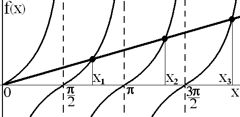
Region III represents a very special case, where the mean field polarization vanishes and the energy of the liquid is determined by thermal fluctuations. The geometry dependent part of the free energy leads to the interaction between the boundaries exactly in the way electromagnetic field fluctuations lead to appearance of the Casimir forces [14]. To describe the fluctuations, we use Eqs. (2)-(3), keeping only terms $\sim s^{2}$. The free energy of the liquid takes a form $G=\left\langle\boldsymbol{s}\left|\widehat{H}\right|\boldsymbol{s}\right\rangle$, where $\widehat{H}$ is a properly constructed self-conjugated operator. Diagonalization is produced by the decomposition $\boldsymbol{s}=\sum_{n}c_{n}\boldsymbol{s}_{n}$ over the complete set of orthogonal and normalized eigen-mode functions $\{\boldsymbol{s}_{n}\}$, so that $G=\sum_{n}k_{n}^{2}|c_{n}|^{2}$, where $k_{n}^{2}$ are the eigen-numbers of $\widehat{H}$ corresponding to the modes $\boldsymbol{s}_{n}$ and enumerated by the index $n$. Each $c_{n}$ is an independent variable.

In the case of the two plane surfaces separated by the distance $d$, the liquid is translational invariant along the interfaces surfaces and the mode functions can be represented in the form $\boldsymbol{s}_{n}=\left(u_{n}\left(z\right),0,v_{n}\left(z\right)\right)\exp e^{ipx}$. The solutions are characterized by the set of numbers $n=\left(\boldsymbol{p},P,m\right)$, where $\boldsymbol{p}$ is the two-dimensional wave vector and $P=\pm 1$ is the parity of the function, $u_{n}\left(-z\right)=Pu_{n}\left(z\right)$. Depending on the parity, the mode functions $u_{n}(z)$ and $v_{n}(z)$ are the linear combinations of $\sin q_{m}^{(1,2)}z$ and $\cos q_{m}^{(1,2)}z$, where $q_{m}^{(1)}=\sqrt{k_{n}^{2}-p^{2}-A}$ and $q_{m}^{(2)}=\sqrt{q_{m}^{2}-4\pi}$. In the practically important case $d\gtrsim R_{D}$, all the terms containing $q_{m}^{(2)}$ are small, $\sim\exp(-d/R_{D})$, and as such can not contribute to the interaction force. This is because at sufficiently large distances from the surfaces only the so-called “force-less”, $\boldsymbol{E}_{P}=0$, fluctuations of the liquid contribute to thermodynamic functions [9]. The wave vector $q_{m}\equiv q_{m}^{(1)}$ is the solution of the characteristic equation: $f\left(X_{m}\right)=aX_{m}$, where $X_{m}=q_{m}d/(2\sqrt{C})>0$, and $a=2\sqrt{C}/(\alpha_{0}d)$. The function $f\left(X\right)$ has the period $\pi/2$ and is obtained by a periodic shift of $\pi/2$ of the main branch of tangent function, $\tan X$ for $-\pi/2<X<\pi/2$, as shown on Figure 2.

The equilibrium free energy of the system is

and, exactly as in the calculation of Casimir energy, formally diverges. To compute the sum, we formally write

Now we can follow [15] and perform the summation using the Cauchy’s argument principle. After the regularization, $G_{eq}\left(d\right)\rightarrow G_{eq}\left(d\right)-G_{eq}\left(\infty\right),$ we derive the expression:

where $y_{0}=d/2L_{T}$ is the dimensionless distance, and $\lambda$ is a material dependent quantity (in Region III $\mu/\alpha_{0}>1$). In the two most important limiting cases, the interaction energy takes form

corresponding to the attraction. This means that the interaction is universal, the dependence on the material constants is weak and can only be found at intermediate distances $d\sim L_{T}$.

The attraction of hydrophobic bodies in our model has an entropic nature, in accordance with earlier predictions [16, 17]. Hydrophobic surfaces order molecules of water and the effects of the molecular ordering in (2) manifests itself in two different ways: from the entropy contribution to $V(\mathbf{s}^{2})$, as in our case, or through the Oseen energy term, modeling the hydrogen bonding. The latter describes the short-range forces and decays at distances $\sim R_{D}$. Hence, for small bodies of sizes $\lesssim R_{D}$ the hydration energy is proportional to the volume [17, 16]. The longer range interaction between hydrophobic bodies at distances $\sim L_{T}$ originates from the long-range dipole-dipole interaction between the molecules and thus requires a complete model like (2)-(3), which naturally includes both distance scales.

On a side note, we predict that under specific conditions there could be a special limit. When the liquid interfaces fail to polarize water molecules, the fluctuations of molecular polarization become strong and the interaction becomes very weak but attractive. The fluctuations may also be relevant next to hydrophobic interfaces, where the mean field ordered state of the liquid may break in a BKT-like phase transition [11, 18], which have been observed in molecular dynamics calculations for the hydration water layers [19].

In summary, we find the polar liquid phenomenology (2)-(3) earlier proposed [9, 10, 11] paints a very physically rich picture of possible wetting regimes and interactions. If used to calculate the interactions between the hydrophilic planes, the model can be considered as the natural improvement of ideas [4, 6, 20, 21, 22, 23, 24]. Our model generalizes the order parameter (the net polarization of the water molecules) in a form useful both for hydrophobic and hydrophilic interfaces, correctly predicts the sign and the distance dependence of the interaction forces depending on the properties of the surfaces. We show that the interactions originate from the fundamentally non-linear and non-local polarizability of the liquid. Our model is characterized by two scales, $R_{D}$ and $L_{T}$, instead of a single scale $\sim R_{D}$ from [6, 7, 8]. The experimental observation of both decay lengths in [1] and [2, 3] together with the prediction [10, 25] and subsequent experimental observation of the ferroelectric features in the bulk liquid water near the $\lambda-$point [12, 26, 27] shows both general consistency and applicability of the model for realistic calculations of macroscopic bodies interactions in water. This observation makes our model the minimal continuous model capable of predicting finer effects depending both on the hydrogen-bond network properties and the electrostatic interactions of the water molecules.

The authors are grateful to Prof. V.G. Levadny for the fruitful discussions. Quantum Pharmaceuticals supported this work.

References

- [1] D. LeNeveu, R. Rand, and V. Parsegian, Nature 259, 601 (1976).
- [2] R. M. Pashley, P. M. McGuiggan, B. W. Ninham, D. F. Evans, et al., Science (New York, NY) 229, 1088 (1985).
- [3] P. M. Claesson and H. K. Christenson, The Journal of Physical Chemistry 92, 1650 (1988).
- [4] S. Marcelja and N. Radic, Chemical Physics Letters 42, 129 (1976).
- [5] R. Kjellander and S. Marčelja, The Journal of Chemical Physics 82, 2122 (1985).
- [6] M. Belaya, M. Feigel’Man, and V. Levadny, Chemical Physics Letters 126, 361 (1986).
- [7] A. Kornyshev and S. Leikin, Physical Review A 40, 6431 (1989).
- [8] S. Leikin and A. Kornyshev, The Journal of Chemical Physics 92, 6890 (1990).
- [9] P. Fedichev and L. Menshikov, arxiv preprint cond-mat/0601129 (2006).
- [10] L. Menshikov and P. Fedichev, Russian Journal of Physical Chemistry A, Focus on Chemistry 85, 906 (2011), arXiv:0808.0991.
- [11] L. Menshikov and P. Fedichev, Journal of Structural Chemistry 50, 97 (2009).
- [12] P. Fedichev, L. Menshikov, G. Bordonskiy, and A. Orlov, JETP Letters 94, 401 (2011), arxiv preprint arXiv:1104.1417.
- [13] A. Kohlmeyer, C. Hartnig, and E. Spohr, Journal of Molecular Liquids 78, 233 (1998).
- [14] H. B. Casimir, in Proc. K. Ned. Akad. Wet (1948), vol. 51, p. 793.
- [15] T. H. Boyer, Annals of Physics 56, 474 (1970).
- [16] D. M. Huang, P. L. Geissler, and D. Chandler, The Journal of Physical Chemistry B 105, 6704 (2001).
- [17] D. Chandler, Nature 437, 640 (2005).
- [18] A. Y. Vasiliev, A. Tarkhov, L. Menshikov, P. Fedichev, and U. R. Fischer, arXiv preprint arXiv:1303.4915 (2013).
- [19] A. Oleinikova, I. Brovchenko, N. Smolin, A. Krukau, A. Geiger, and R. Winter, Physical Review Letters 95, 247802 (2005).
- [20] R. Ramirez, R. Gebauer, M. Mareschal, and D. Borgis, Physical Review E 66, 31206 (2002).
- [21] H. Gong and K. Freed, Physical Review Letters 102, 57603 (2009).
- [22] C. Azuara, H. Orland, M. Bon, P. Koehl, and M. Delarue, Biophysical Journal 95, 5587 (2008).
- [23] P. Koehl, H. Orland, and M. Delarue, Physical Review Letters 102, 87801 (2009).
- [24] D. Beglov and B. Roux, J. Phys. Chem. B 101, 7821 (1997).
- [25] P. Fedichev and L. Menshikov, Pis’ma v Zhurnal Eksperimental’noi i Teoreticheskoi Fiziki 97, 241 (2013).
- [26] G. Bordonskiy, A. Gurulev, A. Orlov, and K. Schegrina, arxiv preprint arXiv:1204.6401v1 (2012).
- [27] G. Vasiliev and A. Orlov, arXiv preprint arXiv:1303.4873 (2013).