CPHT-RR028.0413
QCD description of charmonium plus light meson production in annihilation
B. Pire1, K. Semenov-Tian-Shansky2aa a e-mail:kirill.semenov@polytechnique.edu , L. Szymanowski3.
1CPhT, École Polytechnique, CNRS, F-91128 Palaiseau, France
2IFPA, département AGO, Université de Liège, 4000 Liège, Belgium
3 National Centre for Nuclear Research (NCBJ), Warsaw, Poland
August 24, 2026
Abstract:
The associated production of a and a meson in antiproton-nucleon annihilation is studied in the framework of QCD collinear factorization. In this approach, a hard subprocess responsible for the production of the heavy quark-antiquark pair factorizes from soft hadronic matrix elements, such as the antiproton (nucleon) distribution amplitude and the nucleon-to-pion (antiproton-to-pion) transition distribution amplitude. This reaction mechanism should dominate the forward and backward kinematical regions, where the cross sections are expected to be measurable in the set-up of the P̄ANDA experiment at the GSI-Fair facility.
1 Introduction
The factorization of exclusive amplitudes in a short distance dominated part which may be calculated in a perturbative way in the one hand, and universal confinement related hadronic matrix elements in the other hand, is a welcome feature of quantum chromodynamics (QCD) for specific processes in specific kinematics. The textbook example of such a factorization is nearly forward deeply virtual Compton scattering where generalized parton distributions (GPDs) are the relevant hadronic matrix elements. The extension of this description to other processes such as backward virtual Compton scattering and backward meson electroproduction, has been advocated [1, 2, 3] - although not proven. In the latter process, new hadronic matrix elements of three quark operators on the light cone, the nucleon-to-meson transition distribution amplitudes (TDAs), appear which shed a new light on the nucleon structure, and enable to quantify nucleon’s mesonic cloud. The validity of such a factorization requires at least the existence of a large scale , which has been taken as the spacelike, respectively timelike, virtuality of the photon quantifying the electromagnetic probe in the case of electroproduction, respectively lepton pair emission in antinucleon-nucleon annihilation. This large scale ensures the validity of the perturbative expansion of the hard subprocess with the QCD coupling constant taken at a scale . The factorization scale is also to be taken of order .
In many instances (jet production, heavy meson production or decays…) it has been shown that the occurrence of a heavy elementary particle, for instance a quark with mass , is sufficient to ensure the reliability of a perturbative expansion with . The pioneering studies of the charmonium decay width and of specific charmonium decay channels [4, 5, 6] have proven the value of this approach. We will follow this line of reasoning in the present Letter.
The spectroscopy of charmonium states is at the heart of the physics program of the P̄ANDA experiment at the GSI-Fair facility [7, 8]. Some of these unknown (or badly known) states will decay in a lower mass charmonium such as the and a few ordinary mesons. When scrutinizing the final states produced, it will be of the utmost importance to separate these associated charmonium-light meson states from a background where the light meson(s) just evaporate from the beam or the target nucleon. These latter cases are the target of our study. But we stress that their production process is much more interesting than a mere background to subtract: it is indeed a new way to access the inner structure of the nucleon through the study of baryon to meson transition distribution amplitudes. For definiteness, we will present the study in the case of a single meson produced in conjunction with the . A slight extension of the same formalism applies in the cases where another meson, e.g. or a pair of mesons, e.g. , is produced.
An alternative description of annihilation in a charmonium accompanied by a meson proposed in the literature is the use of effective hadron exchange models; see e.g. [9] and [10, 11]. This method provides an essentially non-perturbative description of the process. Our aim is to single out with the help of factorization techniques the perturbative part of the process and to relate the remaining non-perturbative part to universal fundamental quantities with interpretation within QCD as the light-cone matrix elements of correlators of the fundamental fields.
2 Kinematics
The study of charmonium exclusive hadronic decays has been for a long time one of the fields of application of perturbative QCD methods. It has been argued [12, 5] that the dominating mechanism is the pair annihilation into the minimal possible number of gluons which then produce quark-antiquark pairs forming the outgoing hadrons.
In the present Letter we extend the same perturbative QCD framework for the description of a cross channel reaction in which nucleon-antinucleon annihilate producing heavy quarkonium together with a light meson (, , , ) almost collinear either with incoming nucleon or antinucleon. For simplicity below we address the case of meson and consider the reaction
| (1) |
Here the center-of-mass energy squared and the charmonium mass squared introduce the natural hard scale. In the complete analogy with our analysis [13, 14] we assume that this reaction admits a factorized description within two distinct kinematical regimes (see Fig. 1):
- •
the near-forward kinematics ; it corresponds to the pion moving almost in the direction of the initial antinucleon in center-of-mass system (CMS);
- •
the near-backward kinematics corresponding to the pion moving almost in the direction of the initial nucleon in CMS.
The suggested reaction mechanism forms the distinct forward and backward peaks of the differential cross section of the reaction (1) as the function of ( is the pion scattering angle in the CMS). The process (1) allows us to test the universality of TDAs that appear also in the description of and reactions [15, 14].
Due to the -invariance of strong interaction there exists a perfect symmetry between the forward and backward kinematics regimes of the reaction (1). These two regimes can be considered in exactly the same way (see the discussion in Appendix C of Ref. [14]). Precisely, the amplitude of the reaction (1) within the -channel factorization regime can be obtained from that within the -channel factorization regime with the obvious change of the kinematical variables:
| (2) |
However, the backward and the forward regimes are treated somewhat unequally within the P̄ANDA experimental set-up operating antiproton beam. Indeed, once switching to the laboratory system (which corresponds to the nucleon at rest) one may check that the forward peak of the cross section as the function of is narrowed, while the backward peak is broadened by the effect of the Lorentz boost from the CMS to the laboratory frame.
In this Letter we have chosen to present explicitly the details of calculation of the reaction amplitude within the backward kinematics regime. As usual, the axis is chosen along the colliding nucleon-antinucleon with the positive direction defined by that of the antinucleon beam. We introduce the light-cone vectors satisfying . The Sudakov decomposition of the relevant momenta is presented in the Appendix A of [14].
For the calculation of the hard part of the amplitude we apply the collinear approximation. We neglect both the nucleon and pion masses and assume , where the transverse direction is defined with respect to the direction.
The Sudakov decomposition employed for the calculation of the hard part then reads:
| (3) |
Here is the -channel skewness variable
| (4) |
Following [12], in our calculation we set
| (5) |
taking the average value .
Let us emphasize that we keep the exact kinematics (see Appendix. A of Ref. [14]) for the nucleon spinors and for polarization vector. The physical kinematical domain for the reaction (1) in the backward regime is determined by the requirement , where
| (6) |
where () stands for the nucleon (pion) mass. The limiting value corresponds to
| (7) |
In the calculations presented below we neglect the pion mass .
3 Hard amplitude calculation for
The calculation of scattering amplitude follows the same main steps as the classical calculation of the amplitude [12, 5, 16]. Assuming the factorization of small and large distance dynamics the hard part of the amplitude is computed within perturbative QCD. Large distance dynamics is encoded within the matrix elements of QCD light-cone operators between the appropriate hadronic states. The leading order amplitude of (1) is then given by the sum of the three diagrams presented on Figure 2.


Below we present our conventions for the relevant light-cone matrix elements encoding the soft dynamics. For definiteness we consider the case of the leading twist TDA. The case of TDA is completely analogous. Throughout this Letter we make use of the parametrization of [17]11 1 The relation between this parametrization and the one employed in Refs. [18, 15, 14] is given in the Appendix A of [15]. since it simplifies considerably for case. The parametrization involves invariant functions each being the function of three longitudinal momentum fractions , skewness variable , momentum transfer squared as well as of the factorization scale :
| (8) |
Here MeV is the pion weak decay constant and determines the value of the nucleon wave function at the origin. Throughout this paper we adopt Dirac’s “hat” notation ; ; ; is the charge conjugation matrix and is the large component of the nucleon spinor. For just three invariant amplitudes , and survive in the parametrization (8).
For the leading twist antinucleon DAs we employ the standard parametrization [5] (see also Appendix B of Ref. [14]). The non-relativistic light-cone wave function of heavy quarkonium is given by [5]
| (9) |
where is the -quark mass and stands for the charmonium polarization vector. With the use of the non-relativistic wave function (9) we tacitly assume that each charm quark carries half of the momentum of the . The normalization constant is extracted from the charmonium leptonic decay width :
| (10) |
Using the values quoted in [19] we get
| (11) |
The leading order amplitude of (1) reads
| (12) |
where and stand for the nucleon Dirac spinors. The calculation of diagrams presented on Fig. 2 yields the following result for :
| (13) |
where
| (14) |
For we get
| (15) |
The overall factor in (12) is expressed as:
| (16) |
where stands for the strong coupling. One may check that the poles in are indeed located either on the cross over trajectories , which separate the DGLAP-like and ERBL-like support regions of TDAs22 2 For the definition of the ERBL-like and DGLAP-like support regions of TDAs see [20]., or within the DGLAP-like support region (for the -dependent poles in ) as it certainly should be.
4 Estimates of the cross section
The squared amplitude (12) averaged over spins of initial particles reads
| (21) |
At the leading twist only the transverse polarization of is relevant. To sum over the transverse polarization we employ the relation:
| (22) |
and get
| (23) |
The leading twist differential cross section of then reads [21]
| (24) |
where .
In order to get a rough estimate of the cross section we use the simple nucleon exchange model for TDAs suggested in [15]. We do not expect that the inclusion of the spectral part for TDAs [20] would be essential to draw a conclusion on the feasibility of the relevant experiment and may be postponed until the precise experimental data will be available.
For the TDAs within the parametrization (8) the nucleon pole model of Ref. [15] reads
| (25) |
and
| (26) |
Here , and stand for the nucleon DAs; is the pion-nucleon phenomenological coupling and
| (27) |
ensures the pure ERBL-like support of TDAs. For the simple nucleon pole model (25)
| (28) |
where is given by eq. (19).
As the phenomenological input for our cross section calculation we may use different solutions for the leading twist nucleon DA. Similarly to the case of charmonium decay width our result depends strongly on the form of input nucleon DA. In order to be able to characterize this dependence we present in Table 1 the predictions of decay width (20) into within the pQCD description with the use of the nucleon DAs in question as the numerical input. Several points are to be mentioned.
- •
The decay width (20) shows strong dependence on : . There is no unique opinion in the literature on the value of the strong coupling for the gluon virtuality in question.
- •
Nucleon DAs that are strongly concentrated in the end-point regions such as Chernyak-Ogloblin-Zhitnitsky (COZ) [16] or King and Sachrajda (KS) [22] for seem to overestimate the experimental width by the factor . They require smaller values of to reproduce the experimental value. These solutions have been strongly criticized in the literature (see e.g. discussion in Chapter 4 of Ref. [23]).
- •
The ”heterotic” DA model [24] requires even smaller values of to reproduce the experimental width.
- •
On the other hand, the phenomenological solutions for the nucleon DA which are close to the asymptotic form (Bolz-Kroll (BK) [25], Braun-Lenz-Wittmann (BLW NLO) model of [26]) for underestimate the experimental value of the decay width by a factor . Usually, is required to reproduce the experimental value of .
| for which | |||
| DA model | GeV2 | (KeV) | |
| for | is reproduced | ||
| COZ | 0.42 | 0.26 | |
| KS | 0.84 | 0.24 | |
| “Heterotic” model | 1.20 | 0.22 | |
| BK | 0.05 | 0.38 | |
| BLW NLO | 0.02 | 0.44 | |
| Asymptotic | 0.015 | 0.46 | |
| Experiment | – | – |
Based on the above arguments we have chosen to present our results for the cross section with the value of fixed by the requirement that the given phenomenological solution reproduces the experimental decay width. On Fig. 3 we show our estimates of the differential cross section for as a function of for . On Fig. 4 we show the differential cross section for as a function of for several values of .


The pion scattering angle in the CMS for the -channel factorization regime then can be expressed as:
| (29) |
where
| (30) |
One may check that for indeed , which means backward scattering. Expressing our cross sections as functions of (29) we reproduce the order of magnitude ( pb/GeV2 for ) of the corresponding cross sections presented in [11]. This fact is certainly not surprising since it can be seen as an artefact of a simple nucleon pole model of TDAs.
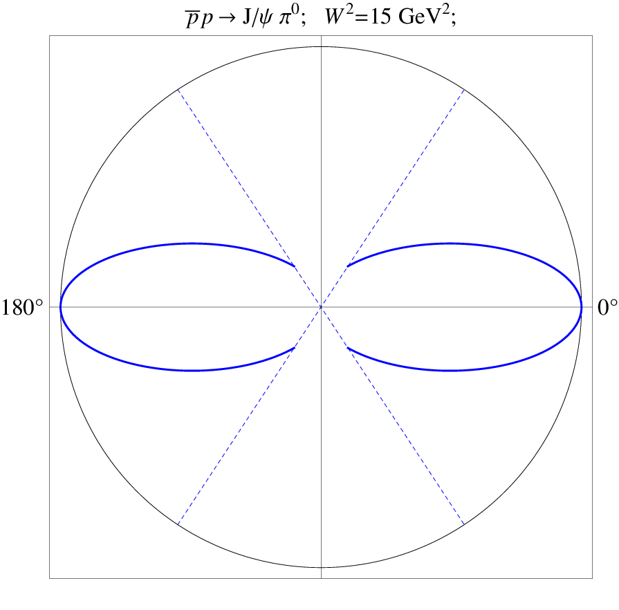
We also reproduce the characteristic shape of angular distributions of the cross sections presented in [11]. On Fig. 5 we show the center of mass angular distribution for the cross section for both forward and backward factorization regimes presented on the polar plot with the polar angle being the pion CMS scattering angle . We present the ratio
| (31) |
as the function of showing the result for GeV2 and for , where is the limiting value (7) of the momentum transfer squared. The left half of the graph corresponds to the near-backward factorization regime and right half of the graph corresponds to the near-forward factorization (see Fig 1). With the dashed lines we show the effect of the cutoff GeV2 for the values of the CMS scattering angle.
Since these rates are certainly within the experimental reach of the P̄ANDA experiment, the study of reaction (1) will provide a valuable universality test for the TDA approach since the same TDAs also arise in the description of [14] and backward pion electroproduction off nucleon [15].
It is worth mentioning that it might be advantageous also to study the process
| (32) |
In our simple nucleon pole model for TDAs the corresponding cross sections are enhanced by the factor due to the isotopic factor in (26).
5 Conclusions
In this Letter we address the reaction which will be studied in the P̄ANDA experiment at GSI-FAIR to look for exotic charmonium states production [27]. We argue that outside the region specific for the resonance production, this reaction may be analyzed within the pQCD framework. It will not only help to quantitatively disentangle resonance production from the universal hadronic background but also will provide valuable information on hadronic structure encoded in nucleon-to-pion TDAs.
Nucleon-to-pion TDAs are essentially non-diagonal matrix elements of QCD light-cone operators which probe the non-minimal Fock state contents of hadrons. Therefore TDAs supply complementary information with respect to diagonal partonic distributions (PDFs, GPDs). On the other hand, the suggested possibility of description of the process in terms of fundamental degrees of freedom of QCD largely increases its theoretical importance. It is also worth mentioning the possible generalization of our approach both to the case of other heavy quarkonium states as well as to various accompanying light meson species (, , , etc.). The TDA framework has also been recently [28] used in a double handbag description of proton-antiproton annihilation into a heavy meson pair.
Within the kinematical range accessible at P̄ANDA we provide the predictions using a simple nucleon pole model for TDAs. The obtained values of cross sections give hope of experimental accessibility of the reaction. Our predictions are consistent with the recent estimates of [11] obtained within a fully non-perturbative effective hadronic theory. However, the latter approach lacks the direct relation to the dynamics of fundamental degrees of freedom of QCD. Precise experimental data, and the study of polarization observables not discussed here, will allow to discriminate between the QCD and hadronic approaches.
It is also worth mentioning that the mass of the charm quark may not be large enough for our leading order (in ) and leading twist analysis to be sufficient to describe the data. More work is certainly needed to go beyond the Born approximation for the hard amplitude, in particular because the timelike nature of the hard probe is often accompanied by large corrections [29].
We acknowledge useful discussions with J.P. Lansberg and are grateful to V. L. Chernyak for correspondence. This work is supported in part by the Polish Grant NCN No DEC-2011/01/D/ST2/03915, the Joint Research Activity Study of Strongly Interacting Matter (acronym HadronPhysics3, Grant 283286) under the Seventh Framework Programme of the European Community and by the COPIN-IN2P3 Agreement.
References
- [1] L. L. Frankfurt, P. V. Pobylitsa, M. V. Polyakov and M. Strikman, Phys. Rev. D 60 (1999) 014010; [arXiv:hep-ph/9901429]; L. Frankfurt, M. V. Polyakov, M. Strikman, D. Zhalov and M. Zhalov, arXiv:hep-ph/0211263.
- [2] B. Pire and L. Szymanowski, Phys. Rev. D 71, 111501 (2005) [hep-ph/0411387].
- [3] B. Pire and L. Szymanowski, Phys. Lett. B 622, 83 (2005) [arXiv:hep-ph/0504255].
- [4] G. P. Lepage and S. J. Brodsky, Phys. Rev. D 22, 2157 (1980).
- [5] V. L. Chernyak and A. R. Zhitnitsky, Phys. Rept. 112, 173 (1984).
- [6] V.L. Chernyak and I.R. Zhitnitsky, Nucl. Phys. B 246, 52 (1984).
- [7] M. F. M. Lutz et al. [PANDA Collaboration], arXiv:0903.3905 [hep-ex].
- [8] U. Wiedner, Prog. Part. Nucl. Phys. 66, 477 (2011) [arXiv:1104.3961 [hep-ex]].
- [9] M. K. Gaillard, L. Maiani and R. Petronzio, Phys. Lett. B 110, 489 (1982).
- [10] T. Barnes, X. Li and W. Roberts, Phys. Rev. D 81, 034025 (2010) [arXiv:1001.1335 [hep-ph]].
- [11] Q. -Y. Lin, H. -S. Xu and X. Liu, Phys. Rev. D 86, 034007 (2012) [arXiv:1203.4029 [hep-ph]].
- [12] S. J. Brodsky and G. P. Lepage, Phys. Rev. D 24, 2848 (1981).
- [13] J. P. Lansberg, B. Pire and L. Szymanowski, Phys. Rev. D 76, 111502 (2007) [arXiv:0710.1267 [hep-ph]].
- [14] J. P. Lansberg, B. Pire, K. Semenov-Tian-Shansky and L. Szymanowski, Phys. Rev. D 86, 114033 (2012) [arXiv:1210.0126 [hep-ph]].
- [15] J. P. Lansberg, B. Pire, K. Semenov-Tian-Shansky and L. Szymanowski, Phys. Rev. D 85, 054021 (2012) [arXiv:1112.3570 [hep-ph]].
- [16] V. L. Chernyak, A. A. Ogloblin and I. R. Zhitnitsky, Z. Phys. C 42, 583 (1989) [Yad. Fiz. 48, 1398 (1988)] [Sov. J. Nucl. Phys. 48, 889 (1988)].
- [17] J. P. Lansberg, B. Pire and L. Szymanowski, Phys. Rev. D 75, 074004 (2007) [Erratum-ibid. D 77, 019902 (2008)] [hep-ph/0701125].
- [18] B. Pire, K. Semenov-Tian-Shansky, L. Szymanowski, Phys. Rev. D 84, 074014 (2011) [arXiv:1106.1851 [hep-ph]].
- [19] J. Beringer et al. (Particle Data Group), Phys. Rev. D 86, 010001 (2012).
- [20] B. Pire, K. Semenov-Tian-Shansky and L. Szymanowski, Phys. Rev. D 82, 094030 (2010) [arXiv:1008.0721 [hep-ph]].
- [21] V. I. Borodulin, R. N. Rogalev and S. R. Slabospitsky, hep-ph/9507456.
- [22] I. D. King and C. T. Sachrajda, Nucl. Phys. B 279, 785 (1987).
- [23] N. Brambilla et al. [Quarkonium Working Group Collaboration], hep-ph/0412158.
- [24] N. G. Stefanis, Eur. Phys. J. direct C 7, 1 (1999).
- [25] J. Bolz and P. Kroll, Z. Phys. A 356, 327 (1996) [hep-ph/9603289].
- [26] V. M. Braun, A. Lenz and M. Wittmann, Phys. Rev. D 73, 094019 (2006) [hep-ph/0604050].
- [27] S. K. Choi et al. [BELLE Collaboration], Phys. Rev. Lett. 100, 142001 (2008) [arXiv:0708.1790 [hep-ex]].; M. Ablikim et al. [ BESIII Collaboration], arXiv:1303.5949 [hep-ex]; T. Xiao, S. Dobbs, A. Tomaradze and K. K. Seth, arXiv:1304.3036 [hep-ex]; Z. Q. Liu et al. [Belle Collaboration], arXiv:1304.0121 [hep-ex].
- [28] A. T. Goritschnig, B. Pire and W. Schweiger, Phys. Rev. D 87, 014017 (2013) [arXiv:1210.8095 [hep-ph]].
- [29] D. Mueller, B. Pire, L. Szymanowski and J. Wagner, Phys. Rev. D 86 (2012) 031502 [arXiv:1203.4392 [hep-ph]].