Stable and metastable hard sphere crystals in Fundamental Measure Theory
Abstract
Using fully minimized fundamental measure functionals, we investigate free energies, vacancy concentrations and density distributions for bcc, fcc and hcp hard–sphere crystals. Results are complemented by an approach due to Stillinger which is based on expanding the crystal partition function in terms of the number of free particles while the remaining particles are frozen at their ideal lattice positions. The free energies of fcc/hcp and one branch of bcc agree well with Stillinger’s approach truncated at . A second branch of bcc solutions features rather spread–out density distributions around lattice sites and large equilibrium vacancy concentrations and is presumably linked to the shear instability of the bcc phase. Within fundamental measure theory and the Stillinger approach (), hcp is more stable than fcc by a free energy per particle of about 0.001 . In previous simulation work, the reverse situation has been found which can be rationalized in terms of effects due to a correlated motion of at least 5 particles in the Stillinger picture.
I Introduction
The crystal lattices of monatomic substances are very often of face–centered cubic (fcc), hexagonally close–packed (hcp) or body–centered cubic (bcc) type. Still, it is a formidable problem in statistical mechanics and quantum chemistry to predict the stable crystal structure and its free energy for a given substance. Approximating the particle interactions in this substance by classical two–body potentials makes the problem amenable to a treatment using methods of classical statistical mechanics, most notably Monte Carlo (MC) simulations and (classical) density functional theory (DFT). While the approximation using two–body potentials may not be very accurate for truly atomic substances, the advance in colloid synthesis allows to realize systems with simple two–body potentials to a good degree of approximation, thus colloid suspensions are a perfect model system for investigating freezing in classical statistical mechanics.
For isotropic two–body potentials ( is the center distance between two particles) a substantial amount of knowledge has been gathered. For potentials with a repulsive core the steepness of the core mainly determines the stability of fcc over bcc, with fcc being more stable for steeper cores. This has been investigated for power–law potentials [1] and screened exponentials [2, 3] where the parameters determine the steepness of the potential. In the hard–sphere limit (), fcc appears to be the stable, equilibrium structure and a possible bcc structure is unstable against small shear [4] which is reflected in squared phonon frequencies being negative for certain wave vectors .
For hard spheres, it is a much more delicate issue whether fcc is more stable than other close–packing structures, most notably hcp. Early theoretical work by Stillinger et al. analyzed the free energy of hard disks and fcc and hcp hard sphere crystals in terms of an expansion in the number of contiguous particles (free to move) in an otherwise frozen matrix of particles at their ideal lattice positions [5, 6, 7] (see below). This expansion could be done analytically only for densities in the vicinity of close–packing and, for and (by quite a tour de force), resulted in hcp being more stable than fcc by a free energy difference per particle . However, the individual terms contributing in this series are much larger than this value of . An extension of this method [8] (still only near close–packing) to shows the reverse situation: fcc is more stable than hcp and , but the last term in the series is still larger in magnitude than (about 6 times for fcc and 3 times for hcp). Simulation work confirms the stability of fcc over hcp also for smaller densities (around coexistence). Using a single–occupancy cell (SOC) method, Ref. [9] estimates at a density of (approximately at coexistence, is the hard sphere diameter). In this method, particles are constrained to their Wigner–Seitz cells and the free energy difference is found by integrating the equation of state. The limitations of this method could be overcome by the powerful Monte–Carlo (MC) lattice switch method which allows to compute directly the free energy difference between two different lattice structures [10]. At the result is . Thus the result of the high–density Stillinger series for for the stability of fcc over hcp and the magnitude of the free energy difference is consistent with the MC simulation result at a considerably smaller density. One may tentatively conclude that for all densities the stability of fcc in the hard sphere system is a subtle result of the correlated movement of five and more particles and the effect in the free energy is very small.
In view of this evidence it appears to be very hard to contribute to the theoretical understanding of the stability of fcc over hcp beyond the Stillinger arguments. In this respect, density functional theory (DFT) seems to be the only promising candidate theory. In the general framework of classical DFT crystals are viewed as “self–sustained”, periodic density oscillations of a liquid, which minimize a unique, but in general unknown free energy functional. Ramakrishnan and Yussouff demonstrated [11] that a simple functional, which is Taylor–expanded about a homogeneous liquid state near coexistence semi–quantitatively accounts for the freezing transition in the hard sphere system. Such Taylor–expanded functionals can be devised for a wide range of two–particle potentials but they are often not very precise. Nevertheless they are a useful starting point for deriving more coarse–grained models via gradient expansions leading to phase field crystal models for materials science [12]. For hard–body potentials there is a constructive way to derive functionals “from scratch” (not relying on perturbative expansions) using essentially geometric arguments. This approach is known as fundamental measure theory (FMT) [13, 14, 15]. With regard to the description of crystals, it has proved to be fruitful to consider the zero–dimensional (0D) limit of density distributions localized to a point and their exactly known free energy [16]. By requiring that the density functional reproduces this 0D free energy for density peaks at one, two and three points in space, a density functional may be constructed which exhibits solid phase properties in very good agreement with simulations [17]. (In the case of density distributions with –peaks at three points, the 0D free energy is reproduced only approximately.)
In the seminal work [17], the crystal density distributions were parametrized with isotropic Gaussians with variable width parameter and normalization (to allow for a finite vacancy concentration ). By minimizing the free energy with respect to the width parameter and the normalization, the following results were obtained: The crystal free energy per particle agrees with simulation to within less than a percent and the Gaussian width is only slightly smaller than seen in simulations. However, furthermore it was found: Z(i) No free energy minimum for and (ii) equal free energies for fcc and hcp. In a study combining simulation and free minimization of FMT functionals [18] it was shown that (i) is a defect of the functional used in [17] (the Tarazona tensor functional) and that upon free minimization the White Bear II tensor functional of Ref. [14] gives thermodynamically consistent results11 1 This is discussed in Ref. [18], Sec. III.A. under the heading “ consistency”. with a small equilibrium vacancy concentration for fcc. The free energies per particle obtained by free minimization vs. constrained minimization using isotropic Gaussians differ by about (near coexistence), which is of the order of magnitude one would also expect for the fcc–hcp difference . Hence one is lead to the suspicion that (ii) (i.e. ) is an artefact of the constrained minimization. This issue will be addressed here.
Apart from the issue of fcc vs. hcp in hard spheres, FMT is also suited to investigate the metastable bcc crystal (which in FMT is simply stabilized by the periodic boundary conditions). A previous FMT study [19] using constrained minimization found two metastable bcc branches as well as a peculiar behavior of the lattice site density peaks when the density is increased. We will investigate this finding further by fully minimizing the FMT functional and will relate our results to the Stillinger series.
II Theory
II.1 Fundamental measure theory
II.1.1 Definition of functionals
In the framework of density functional theory, the grand canonical free energy is a functional of the one-body density profile
| (1) |
where and denote the ideal and excess free energy functionals of the fluid. denotes the chemical potential and the external potential is represented by . The exact form of the ideal part of the free energy is given by
| (2) |
Here, is the de-Broglie wavelength and .
Fundamental measure theory (FMT) currently is the most precise functional for the excess free energy part for the hard sphere fluid. The corresponding excess free energy is given by
| (3) | |||||
| (4) | |||||
Here, is the excess free energy density which is a (local) function of a set of weighted densities with four scalar, two vector and one tensorial weighted densities. These are related to the density profile by the convolutions . The weight functions are given by ( is the hard sphere radius):
| (5) | |||||
By choosing
| (6) |
we obtain Tarazona’s tensor functional [17] based on the original Rosenfeld functional [13]. The choice
| (7) |
corresponds to the tensor version of the White Bear I functional [20]. Finally, with
| (8) |
the tensor version of the white Bear II functional is recovered [14]. This functional is most consistent with respect to restrictions imposed by morphological thermodynamics [21].
In density functional theory, the crystal is viewed as a self–sustained inhomogeneous fluid. Therefore, beside bulk and inhomogeneous fluids, it is possible to study properties of the hard–sphere crystal within the framework of FMT. Using the variational principle, the equilibrium density profile is determined via minimizing the grand canonical free energy functional which leads to the Euler-Lagrange equation:
| (9) |
For the equilibrium crystal, and is lattice–periodic, and , the homogeneous density (bulk density), is fixed by the excess chemical potential . Being computationally simpler than a free minimization of the density profile, crystal density profiles are often obtained by a constrained minimization of a model profile with only a few free parameters such as e.g. a Gaussian profile
| (10) |
Here, the free parameters are the Gaussian peak width and the vacancy concentration .
II.1.2 Choice of unit cells for the numerical solution of Euler-Lagrange equation
Face centered cubic (fcc) and hexagonal close-packed (hcp) are two regular lattices with the highest possible hard–sphere packing fraction (). The body centred cubic (bcc) structure can attain only packing fractions up to . The fcc and hcp structures differ in how sheets of hexagonally packed hard spheres are stacked upon one another. Relative to a reference layer A (see Fig. 1), two other layer types B and C are possible which are laterally shifted with respect to A. In the fcc structure the stacking of the hexagonally–packed planes corresponds to the crystallographic [111] direction and every third layer is the same (ABCABCA) whereas in the hcp lattice ([001] direction), the sequence of A and B repeats (ABABABA) (Fig. 1). If the binding energy (or free energy) were dependent only on the number of nearest-neighbor bonds per atom (bonds have no direction), there would be no energetic difference between the fcc and hcp structures.
The most convenient unit cell for fcc is the cubic unit cell with particles at the corners and 6 face-centred particles (this cell, however, lies oblique in the ABCABCA packing discussed above). For hcp it is the unit cell with hexagonally packed hard spheres on the basal plane. In order to avoid any numerical errors in the comparison between fcc and hcp, we define two extended unit cells of the same size with hexagonally packed spheres as the base plane (see Fig. 1). Discretizing the extended unit cells by the same number of equal–distant grid-points ensures that the lattice points in layer A are on grid points and for layers B and C the lattice points are equally ”off–grid” since there is a mirror reflection symmetry with respect to the –axis between B and C. In view of the narrow density peaks centered around each lattice point, this choice eliminates numerical differences between fcc and hcp free energies to a large extent. In Fig. 1, is the nearest neighbor distance, and in the close-packed case . The fcc cubic symmetry requires which entails that the distance between nearest neighbors within a base plane is the same as between neighboring planes. For hcp, the hexagonal symmetry group does not enforce this constraint, for a discussion of the implications thereof see Sec. III.3 below.

is nearest neighbor distance in the basal plane and is the distance between two neighbouring layers.
II.1.3 Free minimization
We determine the equilibrium crystal profile by a full minimization in three–dimensional real space. The density is discretized over a cuboid volume with edge lengths for bcc (using the cubic unit cell) and and for both fcc and hcp (using the extended unit cells of Fig. 1) with periodic boundary conditions. We perform a double step minimization of the free energy. In the first step, the bulk density and the vacancy concentration are fixed and the Euler–Lagrange equation (9) is solved iteratively with a start profile given by the Gaussian profile (10) with optimal width. The excess chemical potential in Eq. (9) is treated as a Lagrange multiplier to ensure the constraint of fixed . In the next step, this procedure is repeated for different (still keeping fixed), and the equilibrium density profile is determined by minimizing the free energy per particle with respect to the the vacancy concentration, . For a more detailed discussion of this procedure see Ref. [18].
In the program, the density profile and 11 weighted densities (two scalar densities , , three vector densities, , and six tensor densities, ) need to be discretized on a three dimensional grid covering the cuboid boxes. Usually we chose grids for the bcc unit cell with points in the , and directions, respectively, and points for the fcc and hcp extended unit cells. Convolutions in real space are multiplications in Fourier space. The necessary convolutions are computed using Fast Fourier Transformations. We use the FFTW 3.3 library for parallelized Fast Fourier Transforms. The other parts of the code are parallelized through OpenMP.
There are many sophisticated algorithms for minimizing a function and likewise many techniques to increase the speed and efficiency of the process. To have a more efficient algorithm, the iteration of Eq. (9) was done using a combination of Picard steps and DIIS steps (Discrete Inversion in Iterative Subspace) [22]. In order to prevent the procedure from diverging during the Picard iterations, in each step we mix the new density with the old one,
| (11) |
Here, is a mixing parameter and it is usually a small number. For the case of bcc, can be adapted in the course of the iterations in the range of . For fcc and hcp, a constant value for stabilizes the iterations, with values . A typical FMT run consisted of an initial Picard sequence with about steps. Then we alternated between Picard sequence of 7 steps and a DIIS step (which needs another Picard initialization steps), see also Ref. [23].
II.2 Stillinger’s expansion in correlated, contiguous particles
II.2.1 General outline
Consider the canonical partition function for hard spheres:
| (13) | |||||
Here, is the center distance between particles and . We consider a reference lattice of our choice (fcc, hcp or bcc) with lattice sites at positions spanning the volume . We associate each particle with a lattice site at site and that association divides the dimensional configuration space into nonoverlapping regions . The precise form of this association is discussed in Ref. [5], but one may think of it loosely in terms of each particle belonging to the Voronoi cell around site of the lattice. For a chosen subset of lattice sites and associated cells, the index runs over the permutations of the particles among these cells and this leads to an identical division of the configuration space, . The index runs over the different associations of particles with lattice sites and becomes important in the case of finite vacancy concentration. Thus we obtain for the partition function:
| (14) |
For zero vacancy concentration, this decomposition is akin to the SOC method (as e.g. discussed in Ref. [9]) where each particle is confined to its Wigner–Seitz cell. Following Ref. [5], one may write in terms of configuration integrals , , …which describe the correlated motion of one, two, …particles in a background matrix of , , …particles fixed at their associated lattice sites. These configuration integrals are defined as
| (15) | |||||
| (16) | |||||
The integration domains must fulfill , and they depend on the indices of the free particles and also in the index determining at which lattice sites the other particles are fixed. The partition function is now expressed as the product
| (17) | |||||
| (18) |
The s can also be expressed by the recursive relation
| (19) |
where is any proper subset of . (For example, when omitting indices we have and .)
II.2.2 Expansion up to for hcp, fcc and bcc hard spheres
In the following, we restrict calculations to the case (number of particles equal to number of lattice sites), i.e. consider a vacancy–free crystal. From simulations [24] and FMT [18] we can estimate that the effect of vacancies on the free energy of the crystal is small: for fcc hard spheres we have (simulations) and (FMT) in equilibrium at coexistence, the corresponding free energy shift compared to can be estimated from FMT, .
Truncated after the first term, the Stillinger series is
| (20) |
where has been reduced to , the free volume for one particle in a cage of fixed neighbors at their lattice sites. Consequently the free energy is
| (21) |
For fcc and hcp, is equal and has been calculated analytically in Ref. [25], we quote this result in App. A. For bcc, we did not find a literature result and therefore give the calculation and result also in App. A.
The second term in the Stillinger series for gives only a contribution different from 1 if the two fixed particles are neighbors. Thus the truncated Stillinger series is
| (22) |
Here, is the correlated free volume of the two neighboring particles (with dimension (length)6) which may depend on the type of neighbor configuration (index ). The power reflects the freedom to choose the first of the two particles to be any of the particles in the system and is the multiplicity of the neighbor configuration. It is half the number of neighbors of type for a given fixed particle. The associated free energy is
| (23) |
For our considered lattice cases the neighbor types and multiplicities are given in Tab. 1. The cubic lattices fcc and bcc have only one neighbor type whereas for hcp there is a difference whether the neighbor is within the same close–packed plane or in an adjacent close–packed plane. See also Ref. [7] for the multiplicities corresponding to the third term in the series (fcc and hcp).
| lattice | neighbor type | ||
|---|---|---|---|
| fcc | all neighbors | 1 | 6 |
| hcp | within close-packed plane | 1 | 3 |
| in adjacent close–packed planes | 2 | 3 | |
| bcc | all neighbors | 1 | 4 |
We calculate the two–particle volumes for different densities by a simple Monte–Carlo computation. For that we specify a suitably large cuboid volume for each of the two free particles from which sets of random positions (for each of the two particles) are drawn. For each set of random positions overlap is checked with the other particle and the fixed neighboring particle, leading to a total of sets of random positions with no overlap. Then . The statistical error needs to be below for a reliable assessment of the free energy difference between fcc and hcp, and this is achieved with 1000 subsets, each containing sets of random positions. In the limit ( is the close–packing density) agreement was found with the analytical results of Ref. [7], but we had to approach very closely to establish that.
III Results
III.1 Stillinger series
For fcc and hcp, the Stillinger series truncated at gives very good results for the free energy per particle (see Fig. 2, to obtain numbers, we put ). We have compared to very precise simulation data obtained in Refs. [26, 18] which have an error of about . The Stillinger series () results for deviate from these ranging from 0.01 (at ) to 0.03 (at ), this is less than 0.5% relative deviation. This is about the same accuracy we obtain with FMT (see also Ref. [18]). Note, however, that a deviation of the order of 0.01 is about 10 times higher than the fcc–hcp free energy difference obtained from simulations, as discussed before.
For bcc, the situation is very much different. Since the bcc structure for hard sphere is unstable against shear, the crystal can be stabilized in simulations only by constraints such as in the SOC method. We would expect from the previous derivation that the Stillinger expansion is a reasonable series expansion for the free energy of the SOC method. However, as Fig. 2 demonstrates, the first two terms are quite far away from the SOC data and also from the FMT results for the branch with lowest free energy, pointing to the importance of higher correlations. (Ultimately, the shear instability is a collective many–body effect, so perhaps the importance of many–particle correlations also in the constrained crystal is not too surprising.) See, however, the next subsection for a more detailed discussion on bcc solutions within FMT, especially with regard to a solution branch with higher free energy which appears to be linked to the bcc Stillinger solution.
Finally, for fcc/hcp the inclusion of the correlated neighbor term increases the free energy, whereas for bcc it leads to a decrease.

III.2 bcc – FMT results


As already discussed, a bcc crystal solution can only be stabilized by constraints. In FMT, these are the periodic boundary condition on the cubic unit cell. Within the Gaussian parametrization (see Eq. (10)), bcc solutions in FMT (Rosenfeld, Tensor and White Bear Tensor, see Sec. II.1) have been investigated by Lutsko [19] (with the additional constraint , such that in the free energy minimization, the width parameter is the only variable which is varied at a given bulk density ). For small bulk densities (), Lutsko found a single free energy minimum with a rather small width parameter , indicating a broad Gaussian peak. Interestingly, exhibits a maximum at and then decreases again upon increasing the density (i.e. the density peaks become wider upon compressing the crystal!). Moreover, at bulk densities a second free energy minimum was visible (with higer free energy). In this second branch, the width parameter increased (the peak width decreased) with increasing density as one would naively expect.
We investigate these findings further using full minimization. For the first branch with lowest free energy, we confirm that there is a minimal width of the peaks at . Full minimization reveals a rather strong deviation from the simple Gaussian form in the density peaks: The difference in free energy per particle between Gaussian and full minimization is about 0.1 (see Fig. 3 (a)) and thus about 2 orders of magnitude higher than in the case of fcc [18]. Curiously, this free energy difference increases with increasing density beyond . Secondly, the equilibrium vacancy concentration is of the order of 10-2 and thus several orders of magnitude higher than found in fcc. has a minimum at and then increases again, adding to the peculiarities of this solution branch. We note that in an FMT study of parallel hard squares and cubes similar peculiarities have been found [28].
The second branch found by Lutsko is not an artefact of the constrained Gauss minimization. By a careful iteration procedure, we found corresponding fully minimized solutions whose free energy per particle is very close to the values from the Gaussian approximation (thus very much like the fcc solutions and very much unlike the solutions from the first branch), see Fig. 3 (b). For increasing densities, we see a convergence of to the results of the Stillinger series (). Thus the second branch of the bcc solutions has the same character as the fcc solution when compared with the Stillinger approach: only a few correlated particles are sufficient to obtain the free energy.
One could argue that the discussion of these bcc solutions is futile and void of physical significance in view of their overall instability. However, the quality of the FMT functionals and their success in describing the fcc phase leads us to think that these solutions are perhaps not to be discarded altogether. Since around coexistence () the difference in to the fcc crystal is about 0.3 and thus very high, it is reasonable that bcc crystallites have not been observed in the nucleation process of a hard sphere crystal. Nevertheless, the bcc solutions are perhaps a useful reference point for discussing the crossover from fcc to bcc as the most stable crystal structure for other potentials such as of type. These could be treated by suitable perturbation ansatz in the free energy functional. Also, it could be interesting to investigate further the dispersion relation of phonons for the solutions of the first branch and thus shed further light on the shear instability.
III.3 fcc/hcp: Free energy differences and density anisotropies


As discussed in the Introduction, FMT gives the same free energy per particle for fcc and hcp when the Gaussian approximation is employed [17, 19]. Free minimization lifts this degeneracy in the free energy. In order to understand this result qualitatively, it is useful to consider the symmetries in the unit cell of fcc/hcp and the constraints these symmetries place upon the lattice–site density profiles. For fcc, this is best discussed by considering the cubic unit cell in Fig. 4 (a1). The non–radial contributions to the density profile around the lattice point in the origin can be expanded in a Taylor series in where the terms in this series must respect the 48 point symmetry operations in the cubic unit cell (belonging to point group in Hermann–Mauguin notation) [18]:
| (24) |
Here, is an averaged, radial profile which is more or less of Gaussian shape. The leading anisotropic term is of polynomial order 4 with expansion coefficient . One can also understand this result by resorting to an expansion in the subset of spherical harmonics which respect the cubic point symmetry, this leads to an expansion in the so–called Kubic Harmonics [29]. – For hcp, we consider the unit cell in Fig. 4 (a2). The corresponding Taylor expansion for the non–radial contributions to the density profile around the lattice point in the origin has to respect only the 24 point symmetry operations appropriate for the hexagonal group . According to Ref. [30], this leads to
| (25) |
where polynomial terms up to order 3 have been taken into account (with expansion coefficients ). The corresponding construction using spherical harmonics leads to the so–called Hexagonal Harmonics. We observe that there is a qualitative difference in the shape of the density profile between hcp and fcc according to these expansions:
- :
To leading order in anisotropy for hcp, the density peak should look different in –direction (perpendicular to the hexagonally packed planes) than in directions in the – plane. To phrase it differently: one would expect different width parameters for a Gaussian density peak of the form . We did not observe this in our numerical solutions but we will return to this point below.
- :
To next–to–leading order in the anisotropy for hcp, we expect a different behavior when comparing with due to the antisymmetric term in Eq. (25). Such a symmetry breaking is not present in the fcc peak. To demonstrate this difference, we compare , , and between fcc and hcp, see Fig. 4 (b) and (c).22 2 Note that in our numerical computations we used the unit cells depicted in Fig. 4 (a3) (fcc), and in Fig. 4 (a4) (hcp). Thus, the fcc cubic unit cell and the unit cell in Fig. 4 (a3) are related by a three–dimensional rotation. Likewise, the anisotropy expansion for the extended unit cell must be obtained from the corresponding expression (24) for the cubic unit cell by applying this rotation. However, since the density anisotropy is () in Eq. (24), the corresponding density anisotropy must also be () in the rotated unit cell (primes denote the coordinates in the extended unit cell in Fig. 4 (a3)). Indeed we observe that the symmetry is broken for the hcp profile, in accordance with the anisotropy expansion, and we conclude that the fcc/hcp free energy difference in FMT results from this symmetry breaking.
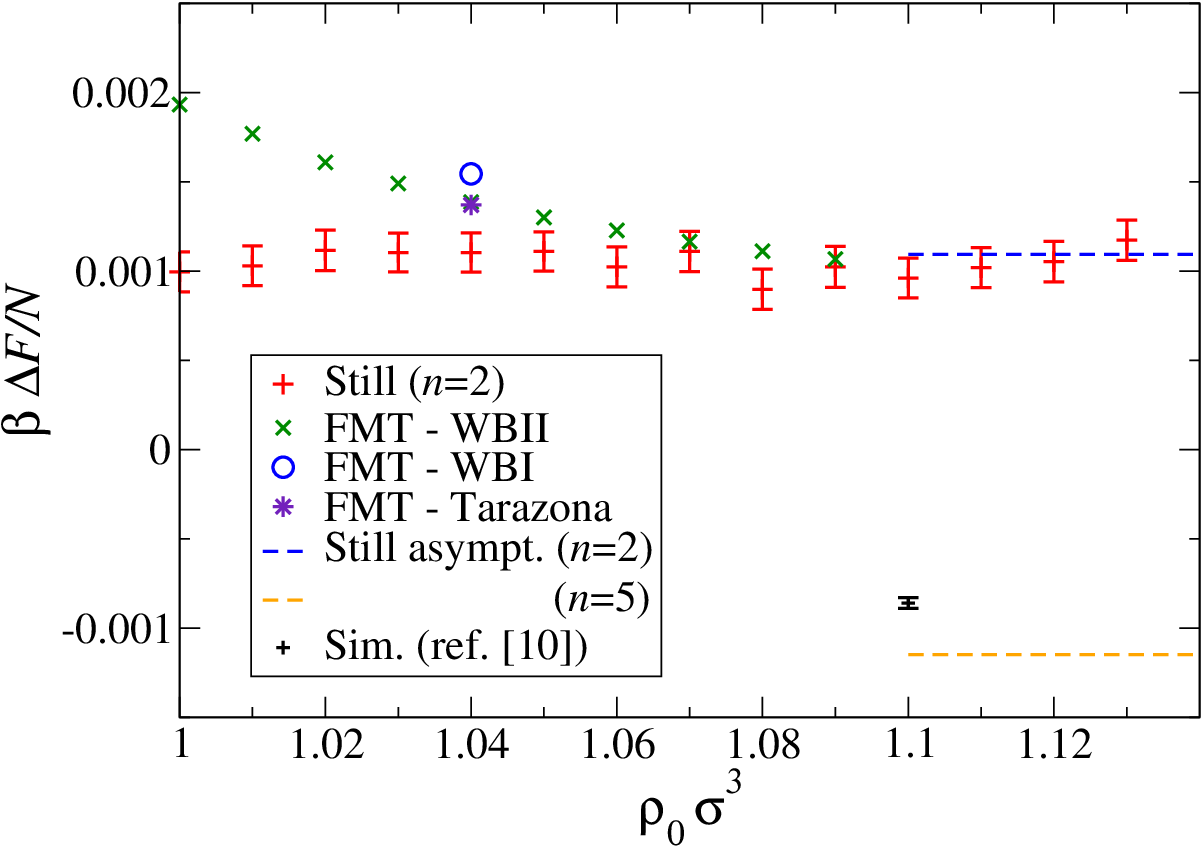
Our results for the fcc/hcp free energy difference per particle are given in Fig. 5(a). In FMT (White Bear II–Tensor), the difference is larger than zero, implying that hcp has lower free energy. Furthermore, there is only a moderate drop of with the bulk density . At coexistence (), we have computed also for other FMT functionals (Tarazona–Tensor, White Bear–Tensor) and found no change in sign but a variation in magnitude by 50% or . In view of the variation of for fcc between the functionals (about , i.e. a factor of 80 larger), the functionals are very consistent with each other with respect to the stability of hcp. The results from the Stillinger series () for are approximately constant () with increasing density and coincide with the analytical value at close packing obtained in Ref. [7]. It is remarkable that also the FMT results seem to converge to this value. – For comparison, in Fig. 5(a) we have also included the analytical value from the Stillinger series () [8] and the simulation value of Ref. [10]. Although FMT does not agree with the sign of obtained in the simulation, it is gratifying to note that according to these results FMT is correct on the level of two correlated particles in the Stillinger picture.
Finally, we return to the observation that in the hcp density anisotropy the leading term (see Eq. (25)) was missing in our numerical solutions. This is related to our choice of the distance between the hexagonally packed layers ( where is the nearest neighbor distance, see Fig. 1). With this choice the distance between nearest neighbors is the same for two sites within the same hexagonally packed planes and two sites in two adjacent planes. However, the hcp symmetry group does not require this, and one is free to choose another distance between the planes. With a different choice, also the nearest neighbor distance is different for sites in two different planes and also the width of the lattice site density profiles will be different in the direction normal to the hexagonally packed planes. We have investigated whether also the free energy minimum for hcp shifts to a value different from . In order to keep the bulk density constant we defined a stretching parameter, , which describes the distortion of the crystal in –direction. In order to keep the bulk density constant, we rescaled the nearest neighbor distance in the planes as follows: . Full minimization was done for a range of values. The result for which minimizes is shown in Fig. 5 and it is seen that the equilibrium distortion is quite small, below . The corresponding free energy shift per particle compared to the solution with is about . These results are actually similar to the ones in Ref. [31]: There, a similar lattice distortion was calculated for the zero–temperature Lennard–Jones hcp crystal by lattice sums.

IV Summary and conclusions
In this work we have performed a study of bcc, fcc and hcp hard sphere crystals using unrestricted minimization in density functional theory (DFT) of Fundamental Measure type (FMT) which is currently the most accurate approach. We have complemented these investigations with an approach which is based on the expanding the crystal partition function in terms of number of free particles while the remaining particles are frozen at their ideal lattice positions (Stillinger series).
For the metastable bcc crystal, we have found two solutions for bcc crystals whose free energies are well above the free energies of fcc/hcp (see Fig. 2 and 3(b)). The first solution (with a rather large density peak width at lattice sites) is characterized by a rather large equilibrium vacancy concentration () and its free energy can not be described by the Stillinger approach. The shear instability of bcc is presumably related to this first solution. The second solution (characterized by a small peak width and small equilibrium vacancy concentrations) agrees well with the solution from the Stillinger approach () with respect to its free energy.
The free energy degeneracy between fcc and hcp, found in previous approaches using constrained, rotationally–symmetric density peaks around lattice sites, is broken upon full minimization. The density asymmetries are qualitatively different for fcc and hcp and agree with expansions in respective lattice harmonics (see Fig. 4). We found that in FMT the free energy per particle is lower for hcp than the one for fcc by about . This agrees remarkably well with the Stillinger solution for (see Fig. 5). Simulations, however, indicate that fcc has a lower free energy than hcp by about the same figure. Previous investigations of the Stillinger approach in the high–density limit (near close packing) have shown that hcp is more stable than fcc for and the situation reverses for . Thus, the stability of fcc seems to be a subtle effect involving the correlated motion of at least 5 particles which currently can not be captured by the FMT functionals.
Appendix A One–particle volumes for the fcc/hcp and bcc hard–sphere crystal
A.1 fcc and hcp
A.2 bcc
In case of bcc the free volume is given by an octahedral–like body (see Fig. 6) centered in the cubic unit cell. The faces are parts of the surfaces of the exclusion spheres (of radius ) around the corners of the cubic unit cell. Let be the side length of the cubic unit cell. The free volume is then given by
| (28) | |||||


References
- [1] R. L. Davidchack and B. B. Laird, Phys. Rev. Lett. 94, 086102 (2005).
- [2] E. J. Meijer and D. Frenkel, J. Chem. Phys. 94, 2269 (1991).
- [3] V. Heinonen, A. Mijailovic, C. V. Achim, T. Ala-Nissila, R. E. Rozas, J. Horbach, and H. Löwen, J. Chem. Phys. 138, 044705 (2013).
- [4] W. G. Hoover, D. A. Young, and R. Grover, J. Chem. Phys. 56, 2207 (1972).
- [5] F. H. Stillinger, Z. W. Salsburg, and R. L. Kornegay, J. Chem. Phys. 43, 932 (1965).
- [6] Z. W. Salsburg, W. G. Rudd, and F. H. Stillinger, J. Chem. Phys. 47, 4534 (1967).
- [7] W. G. Rudd, Z. W. Salsburg, A. P. Yu, and F. H. Stillinger, J. Chem. Phys. 49, 4857 (1968).
- [8] H. Koch, C. Radin, and L. Sadun, Phys. Rev. E 72, 016708 (2005).͒
- [9] L. V. Woodcock, Nature 384, 141 (1997).
- [10] A. D. Bruce, N. B. Wilding, and G. J. Ackland, Phys. Rev. Lett. 79, 3002 (1997).
- [11] T. V. Ramakrishnan and M. Yussouf, Phys. Rev. B 19, 2775 (1979).
- [12] H. Emmerich, H. Löwen, R. Wittkowski, T. Gruhn, G. I. Toth, G. Tegze, and L. Granasy, Adv. Phys. 61, 665 (2012).
- [13] Y. Rosenfeld, Phys. Rev. Lett. 63, 980 (1989).
- [14] H. Hansen–Goos and R. Roth, J. Phys.: Condens. Matter 18, 8413 (2006).
- [15] S. Korden, Phys. Rev. E 85, 411150 (2012).
- [16] P. Tarazona and Y. Rosenfeld, Phys. Rev. E(R) 55, 4873 (1997).
- [17] P. Tarazona, Phys. Rev. Lett. 84, 694 (2000).
- [18] M. Oettel, S. Görig, A. Härtel, H. Löwen, M. Radu, and T. Schilling, Phys. Rev. E 82, 051404 (2010).
- [19] J. F. Lutsko, Phys. Rev. E 74, 021121 (2006).
- [20] R. Roth, R. Evans, A. Lang and G. Kahl, J. Phys.: Condens. Matter 14, 12063 (2002).
- [21] P.-M. König, R. Roth, R. and K. Mecke, Phys. Rev. Lett. 93, 160601 (2004).
- [22] A. Kovalenko, S. Ten-No and F. Hirata, J. Comput. Chem 20, 9, 928-936 (1999).
- [23] M. Oettel, S. Dorosz, M. Berghoff, B. Nestler, and T. Schilling, Phys. Rev. E 86, 021404 (2012).
- [24] C. H. Bennett and B. J. Alder, J. Chem. Phys 54, 4796 (1971).
- [25] R. J. Buehler, R. H. Wentorf, J. O. Hirschfelder, and C. F. Curtiss, J. Chem. Phys. 19, 61 (1951).
- [26] C. Vega and E. Noya, J. Chem. Phys 127, 154113 (2007).
- [27] W. A. Curtin and K. Runge, Phys. Rev. A 35, 4755 (1987).
- [28] S. Belli, M. Dijkstra, and R. van Roij, J. Chem. Phys. 137, 124506 (2012).
- [29] F. von der Lage and H. A. Bethe, Phys. Rev. 71, 612 (1947).
- [30] F. Nizzoli, J. Phys. C: Solid State Phys. 9, 2977 (1976).
- [31] F. H. Stillinger, J. Chem. Phys. 115, 5208 (2001).