Dirac’s discrete hypersurface deformation algebras

Diffeomorphism symmetry is the fundamental gauge symmetry of general relativity, deeply entangled with its dynamics. In the canonical framework this gauge symmetry leads to the Hamiltonian and diffeomorphism constraints. They generate multi–fingered time evolution – that is the equal time hypersurface can be deformed and pushed forward in various ways. These deformations of the hypersurface satisfy a geometric algebra which is reflected in the Poisson algebra of the constraints [1], known as Dirac’s hypersurface deformation algebra [2].

An important goal for the canonical quantization program is to find a quantum representation of the algebra [3, 4, 5]. It has not been reached yet, even in the case of 3D gravity which is a topological theory and is well understood in many of its aspects. The Dirac algebra is universal [1], i.e. it is the same algebra for any theory of hypersurfaces embedded in a higher dimensional manifold. To understand possible quantum representations of this algebra would therefore be beneficial not only for gravity.

One reason that such a representation is still missing, is that many approaches use discretizations either from the outset or as auxiliary structures to e.g. regularize the quantum constraints. However discretizations generically break diffeomorphism symmetry [7, 8, 9], even classically and in simple systems [10, 11]. For instance, the canonical analysis of Regge gravity [12] shows that in this case constraints are replaced by proper evolution equations [13]. In 3D, Regge gravity [14] does however provide a symmetry preserving discretization, which has to be adjusted to the presence of the cosmological constant [15] though. Thus we might hope that a quantum representation of the constraint algebra might be obtainable at least in this case. Indeed quantizations of the constraints are available [16, 17, 18, 19], although a representation of the Dirac algebra, even classically, has not been found so far.

3D quantum gravity [20, 21, 22, 23] had been used as a simplified model for 4D gravity for some time. It can be formulated in a number of ways, in traditional (canonical) ADM form, for instance [23], in Chern–Simons form [22, 24] or as a so–called BF theory, which coincides with the Palatini formulation of 3D gravity.

We will work with the latter version, as it is nearest to the variables and methods used in loop quantum gravity, see for instance [25]. There has been also a considerable amount of work on the loop quantum gravity version of 3D gravity [26, 17, 27, 28, 19]. Most of this work, with the exception of [17] makes use of the fact that the Hamiltonian and diffeomorphism constraints can be recast into the flatness constraints. Whereas the first set satisfies the Dirac algebra of hypersurface deformations, the second set is Abelian.

Despite a good understanding of discrete 3D gravity there is so far no complete discussion or definition of Dirac’s hypersurface deformation algebra for discrete surfaces available. The works [29, 30] are incomplete for various reasons, with [29] arguing (incorrectly) that such an algebra has to be necessarily non–local.

Thus we will provide here an explicit classical realization of the hypersurface deformation algebra for discrete 3D gravity. We discuss the geometric interpretation of the constraints and use these insights to define (various) hypersurface deformation algebras also for discrete 4D gravity (and higher dimensional discretized surfaces). In this case we have however to restrict to the flat sector (or homogeneously curved sector if a cosmological constant is present) of these theories, as otherwise diffeomorphism symmetry will be broken by the discretization. Nevertheless this justifies the hope that some results of the 3D theory can be applied to the 4D case. This might even hold for the quantum theory [31].

The organization of the article is as follows. In the Section 2, we review the continuum formulation of 3D gravity, in particular the Dirac algebra, and we present in the Section 3 the discretization we are going to use, inherited from loop quantum gravity. In the Section 4 we introduce the Hamitlonian and diffeomorphism constraints, using a natural space–time splits coming from the loop quantum gravity fluxes. We discuss the form of the algebra and the main tool for its computation in the Section 5. In the Sections 6 and 7, we give the explicit Poisson brackets between the constraints associated to a single 3-valent vertex and to a face respectively. The hypersurface deformation algebra is written in terms of lengths and dihedral angles in the Section 8. The Section 9 shows that the Thiemann trick, used to define the quantum Hamiltonian in loop quantum gravity (in particular [17]) is also available in the discrete setting, and can be used to write our Hamiltonian constraints. We then move on to higher dimensions, starting with the 4D case in the Section 10, in which we argue that a closed algebra is available in the flat sector of the theory. We introduce the corresponding constraints in the Section 11, which work in arbitrary dimension on the boundary of a $d$-simplex. The constraint algebra is found in the Section 12, and generalized to the case of a non-vanishing cosmological constant (describing homogeneously curved space) in the Section 13. We close the paper with a discussion in the Section 14. The Appendix A provides details on the evaluation of the Poisson brackets for 3D gravity, relevant for the Sections 6 and 7, and the Appendix B contains background material on the affine metric in a simplex that we use in the Sections 11, 12.

3D (Euclidean) gravity can be formulated in first order form, in which the co–triad $e_{\mu}^{k},\,k=1,2,3$ and a connection one–form $A_{\mu}^{k}$ are the basic variables. Here $\mu,\rho,\ldots$ denote space time indices and $i,k,j$ internal ($su(2)$ algebra) indices, which are raised and lowered with the internal Euclidean metric $\delta_{kl}$. With the curvature tensor

the action for a 3D manifold ${\cal M}=\Sigma\times\mathbb{R}$ can be written as

Here $\epsilon^{ab},\epsilon^{\sigma\mu\nu}$ are totally antisymmetric Levi–Civita tensor densities and $\epsilon^{ljk}$ is the Levi–Civita tensor in the internal indices. We use the Einstein summation convention. In the second line in (2.2) we isolated the time components $\mu=0$ from the spatial components $\mu=a,b$, describing the spatial hypersurface $\Sigma$ by $x^{0}=\text{const.}$.

Thus we find the momenta

giving the canonically conjugated pair

The other Poisson brackets vanish: $\{A_{a}^{k}(x),A_{b}^{j}(y)\}=0$ and $\{E^{a}_{k}(x),E^{b}_{j}(y)\}=0$.

The time components of $e,A$ are Lagrangian multipliers for the action (2.2), varying this action with respect to $e_{0}^{j}$ and $A_{0}^{j}$ we find the Gauß  and flatness constraints

where $T^{l}_{\mu\nu}=\partial_{\mu}e^{l}_{\nu}-\partial_{\nu}e^{l}_{\mu}+\epsilon^{ljk}A_{\mu j}e_{\nu k}-\epsilon^{ljk}A_{\nu j}e_{\mu k}$ is the torsion of the connection $A$ and triad $e$.

These constraints are first class forming the (Galilean symmetry) algebra

where ${\cal G}[\Lambda]=\int\Lambda^{j}{\cal G}_{j}d^{2}x$ and ${\cal F}[N]=\int N^{j}{\cal F}_{j}d^{2}x$. The bracket $[A,B]^{k}=\epsilon^{ijk}A^{i}B^{j}$ is the Lie algebra bracket of $su(2)$.

The flatness constraints generate translations in the triad variables $E$ whereas the Gauß constraints generate rotations in the internal space. Gauge symmetries corresponding to diffeomorphisms arise as combinations of the translations and rotations, see for instance [17, 32, 25].

This leads to the following constraint generating spatial diffeomorphisms

and the Hamiltonian constraint

Here $n^{j}$ is the normal to the hypersurface $x^{0}=\text{const.}$

This form of the constraints is the same as the form of the constraints in 4D expressed in (self–dual) Ashtekar variables [33].

The term in (2.7) proportional to the Gauß constraints is often omitted. Again we introduce the smeared constraints

The following Poisson bracket algebra holds modulo terms proportional to Gauß constraints (see for instance [33, 25] for the computation)

Here $q^{ab}$ is the inverse of the two–metric $q_{ab}=e^{k}_{a}e_{bk}$, and $\cal L$ is the Lie derivative.

This Poisson algebra is known as Dirac’s hypersurface deformation algebra and describes the commutator of normal and tangential deformations of a hypersurface. It is universal, i.e. holds in all dimensions and with arbitrary field content. A special feature of the Dirac algebra is the appearance of the structure function $q^{ab}$ in the brackets between two Hamiltonian constraints.

Here we will review shortly the standard choice of discretization for 3D gravity in first order form, [26, 28, 25].

The internal index $k$ in $A_{a}^{k},e_{b}^{k}$ transforms according to the fundamental representation of $SO(3)$, i.e. the spin one representation. This agrees with the adjoint representation on the Lie algebra $su(2)$, which suggest to introduce the Lie algebra valued forms $A_{a}=A^{k}_{a}T^{k}$ and $e_{b}=e_{b}^{k}T^{k}$, where $T^{k}$ is a basis of $su(2)$. We will work with $T_{k}=T^{k}=-\frac{i}{2}\sigma_{k}$ where $\sigma_{k}$ are the Pauli matrices.¹¹ 1 These satisfy $\sigma_{j}\sigma_{k}=\delta_{jk}\mathbf{1}+i{\epsilon_{jk}}^{l}\sigma_{l}$, from which $T_{i}T_{j}=-\tfrac{1}{4}\delta_{ij}\mathbf{1}+\tfrac{1}{2}{\epsilon_{ij}}^{k}T_{k}$ and $T_{i}T_{j}T_{m}=\tfrac{1}{4}\left(\delta_{im}T_{j}-\delta_{ij}T_{m}-\delta_{jm}T_{i}\right)-\tfrac{1}{8}\epsilon_{ijm}\mathbf{1}$ follows.

The parallel transport along a curve $\gamma$ of a Lie algebra valued object $V$ is defined by $V(s)=h(s)V(0)h(s)^{-1}$ where $h(s)$ is the holonomy of the connection $A$ given by

with $A(s)=\dot{\gamma}^{a}(s)A_{a}(\gamma(s))$. A dot denotes differentiation with respect to the curve parameter $s$. Note that with this definition we have for the composition of edges $e_{1}\circ e_{2}$ the relation $h_{e_{1}\circ e_{2}}=h_{e_{2}}h_{e_{1}}$.

Our choice of discretization will replace the connection by holonomies $g_{e}:=h_{e}(1)$ along oriented edges $e$. The triad variables will be encoded into the fluxes

where $e^{*}$ is an edge cutting $e$ transversally and such that $(e,e^{*})$ are positively oriented. Here $h_{e,e^{*}}(s)$ parallel transports vectors from the point $s$ on $e^{*}$ to the source vertex $v_{s}=e(0)$ of $e$. We define $h_{e,e^{*}}(s)$ as follows: Choose the parametrization of the curves $e$ and $e^{*}$ such that the intersection point in both cases corresponds to $s=\frac{1}{2}$. Then

where $h_{e^{*}}(\tfrac{1}{2},s)$ is the parallel transport from the parameter $s$ to the parameter $\tfrac{1}{2}$ along $e^{*}$.

We inserted the holonomies to ensure a local transformation behaviour of the fluxes under internal rotations $E_{e}\rightarrow g(v_{s})\,E_{\gamma}\,g(v_{s})^{-1}$ where $g(\cdot)$ denotes the gauge field on the spatial hypersurface $\Sigma$.

Under the inversion of the orientation of the edge $e\rightarrow\bar{e}:=e^{-1}$ the holonomies and fluxes transform as

The Poisson brackets between holonomies and fluxes can be computed and result [34, 25] in

We can deduce from (3.5) for the bracket with an inverse group element $\{E^{j}_{e}\,,g^{-1}_{e}\}\,=\,-T^{j}g_{e}^{-1}$ as well as the relation $\{E_{\bar{e}}^{k},E^{l}_{e}\}=0.$

The Gauß constraints are assigned to vertices and are represented as

i.e. as sum over the fluxes associated to the outgoing ($e:v_{s}(e)=v$) and the incoming $e:v_{t}(e)=v$ edges at $v$. The Gauß  constraints generate gauge transformations on the internal index, i.e. internal rotations. Later–on, in the Section 8, we will discuss the reduced phase space with respect to the Gauß  constraints.

From the construction of the holonomy and flux variables we can infer the following interpretation. The flux $E_{e}$ gives the components of the edge $e^{*}$ in a frame associated to the source vertex $v_{s}(e)$ of $e$. The holonomy variables $g_{e}$ are used to transport between the frames associated to the source vertex $v_{s}(e)$ and target vertex $v_{t}(e)$ of $e$. Thus the Gauß constraints impose that the fluxes around a vertex sum to zero, which geometrically imposes that the dual edges $e^{*}$ form a closed curve. For a three-valent vertex this will define a closed triangle. (For higher–valent vertices the edges $e^{*}$ making up the piecewise linear curve close, but will in general not span a 2–dimensional subspace.) Due to this interpretation we will assume that the edges and vertices are the elements of a 2–complex, which discretizes the 2D surface $\Sigma$. This latter fact means that we can also identify faces $f$. The 2–complex is usually assumed to arise as the dual of a triangulation (in which case the vertices are three–valent) or more generally a discretization with polygonal cells (which allows higher valent vertices).

The flatness constraints impose that the parallel transport around (contractible) loops is trivial. The most elementary loops are given by the boundaries of the faces. We have furthermore to specify the frame, i.e. vertex, in which the holonomy is expressed. Thus we define the flatness constraints²² 2 We choose a symmetrized form of the constraints, as this is the form that is usually employed in the Hamiltonian constraints. It however also allows for the solution $h_{fv}=-\mathbb{I}$. One can also use $F_{fv}=\mathbb{I}-h_{fv}$ – this will not change the algebra of the constraints. In the following we will understand as constraint hypersurface the subspace defined by $h_{fv}=\mathbb{I}$. as

with $h_{fv}$ the holonomy around a face (dual to a vertex in the triangulation) starting with the edge $e\subset f$ which we assume to have $v$ as a source vertex $v=v_{s}(e)$, i.e. $h_{fv}=\cdots g_{e^{\prime\prime}}g_{e^{\prime}}g_{e}$. In the following, we will often parametrize $\sutwo$ matrices as $h=h^{0}\mathbb{I}+h^{i}T^{i}$, where $h_{i}=-2\tr(hT^{i})$ is the projection of $h$ onto the generator $T^{i}$. The inverse of $h$ writes $h^{-1}=h^{0}\mathbb{I}-h^{i}T^{i}$. Therefore,

As can be easily checked the algebra of flatness and Gauß  constraints is again first class, with the flatness constraints forming an Abelian subalgebra. In the following subsection we will find combinations of these constraints, that can serve as discrete versions of the Hamiltonian and diffeomorphism constraints.

The action of the flatness constraints on the flux associated to $e$ is given by

with the last equation holding on the constraint hypersurface. Again we assume that $h_{f,v}=\cdots g_{e^{\prime\prime}}g_{e^{\prime}}g_{e}$. The action (4.1) of the flatness constraints generalizes to the fluxes $E_{e^{\prime}}$ with $e^{\prime}$ in the boundary of $f$, if these are transported to the reference frame of $v_{s}(e)$. Thus $F_{f,v}$ generates translations in the (to $v$ parallel transported) components $E^{k}_{e^{\prime}}$ of the fluxes associated to the edges $e^{\prime}$ in the boundary of the face $f$. This face $f$ is dual to a vertex $f^{*}$ in the dual triangulation, and we assume that the face is such that $e^{*}$, the dual edge to $e$, points towards the dual vertex $f^{*}$.

Now contract $F_{f,v}$ with a vector $-n^{k}$,

This defines a combination of constraints which according to

generates the translation of $E^{k}_{e}$ by the vector $n^{k}$.

Thus Hamiltonian (and diffeomorphism) constraints may be defined by contracting the holonomy around each face with some choice of normals (and vectors tangent to the hypersurface). However, the holonomy $h_{fv}$ probes the curvature around a vertex of the triangulation and there is no obvious notion of tangent and normal vectors to the vertex. One could proceed with some averaging over the normals of the adjacent triangles. That would require to specify the details of the averaging. The loop quantum gravity version [17] proceeds in another way and associates one Hamiltonian constraint (the diffeomorphisms being treated with a different method) to each dual vertex (corresponding to a triangle in the triangulation). Thus there is an averaging over the three vertices of the triangle and correspondingly of the three holonomies involved. Note that the counting of constraints might not necessarily match up in this case, that is one might obtain a redundant set or an incomplete set. For 4D gravity this discrepancy has been noted in [35], here we see that one should be aware of possible redundancies between the constraints.

Instead of averaging, we will work with an over–complete basis of constraints. Possible averagings can be performed afterwards and the constraint algebra adjusted, which in particular is straightforward if the averaging coefficients are constants.

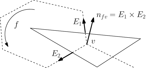
A vertex of the triangulation is shared by at least three triangles. Each of them has a local frame, a basis of which being provided by the two edge vectors of the triangle meeting at the vertex, say $E_{1},E_{2}$, which span the tangential directions to the triangle, and an obvious choice of normal,

In the dual graph, the edge vectors $E_{1},E_{2}$ are equivalently identified by a pair face-vertex $(f,v)$. The face $f$ is dual to the vertex of the triangulation, and the vertex $v$ labels the triangle that provides a local basis. $E_{1},E_{2}$ are the vectors associated to the two dual edges meeting at $v$ in the boundary of $f$. In the definition of the normal (4.4), we have assumed that $E_{1},E_{2}$ are both outgoing (or both ingoing) at $v$. The situation is summarized in the Figure 1.

We can now define a Hamiltonian and diffeomorphism constraints by contracting the holonomy, or rather the flatness constraint $F_{f,v}$ with the appropriate vectors for each pair $(f,v)$,

Here and in the following we will sum over pairs of internal indices, even if these are not in the usual summation convention position (as the internal indices are raised and lowered with the trivial metric $\delta_{kl}$).

To describe the algebra generated by those constraints, it will be very convenient to use the following metric per pair $(f,v)$,

Its determinant is $\det Q=|E_{1}\times E_{2}|^{2}$, so that when $E_{1},E_{2}$ are linearly independent, it has an inverse,

whose matrix elements will be denoted $Q_{fv}^{\alpha\beta}$. Note that this really is the analogue of the continuum inverse 2-metric, which we expect to appear in the Dirac algebra. It naturally induces a ‘space–time split’ as

Here we sum over $\alpha,\beta=1,2$. This identity can be used to decompose any vector $A$ into components tangential to the triangle dual to $v$ and parallel to the normal $n$. In the case of the flatness constraint/holonomy $h^{i}_{fv}$, the components are exactly the diffeomorphism and Hamiltonian constraints,

The constraints are redundant in two ways:

• •

  Local redundancy: The holonomy has three real degrees of freedom, so that the flatness constraints give three constraints per face. We have define three constraints for every face–vertex pair $(f,v)$, which if the two edge vectors associated to $(f,v)$ are linear independent, are also independent. Thus in general the constraints associated to different vertices at the same face can be related to each other.

• •

  Global redundancy: The constraints generate vertex translations of the triangulation (which can be locally embedded into 3D flat space time due to the equations of motion). Given for instance a spherical triangulation, we can translate all vertices at once such that we either produce a global rotation or a global translation. Thus in this case we have six combinations among the vertex translations, which do not change the length and the dihedral angles of the triangulation. The latter provide a parametrization of the Gauß constraint reduced phase space. Thus for the boundary of a tetrahedron one will have 4 (triangulation) vertices, hence 12 (flatness) constraints. Only six of these are independent, fixing the dihedral angles as functions of the lengths [8]. Related is the redundancy between the flatness constraints (on the full phase space) induced by the integrated Bianchi identity. For a spherical surface this identity implies that the holonomy of a given face can be written as a combination of the holonomies of other faces.

The latter global redundancy has been overlooked in [29] and lead there to the conclusion that it would not be possible to obtain a closed (local) hypersurface deformation algebra for discrete geometries. We will show that this is clearly not the case.

The form of the continuum constraint algebra (2.11) can actually be derived by geometrical considerations [1] – it reflects the commutator of deformations of a hypersurface embedded in a higher dimensional manifold. This shows that the algebra is universal, i.e. it is independent from the field content. Moreover, given a certain set of assumptions on the number and metric interpretation of the (ADM) phase space variables, the Hamiltonian and diffeomorphism constraints can be derived uniquely [36]. (This work has been performed in the ADM variables, we are not aware of a derivation in connection or Ashtekar–Barbero variables.)

We will also derive the constraint algebra by geometric considerations, for the boundary of a simplex of arbitrary dimensions, in section 11. Let us shortly explain how the form of the algebra arises.

• (a)

  The commutator of diffeomorphism constraints with diffeomorphism constraints gives again diffeomorphism constraints. This is due to the diffeomorphisms describing deformations in the tangent space to the spatial hypersurface. The commutator does not leave this hypersurface.

• (b)

  The commutator of a Hamiltonian and a diffeomorphism constraint gives a Hamiltonian. The normal to the hypersurface does not change under tangential deformations of this hypersurface. However a tangential vector defining the spatial diffeomorphism changes under a normal deformation – namely by the normal itself. Thus we obtain a Hamiltonian deformation as the commutator.

• (c)

  In (5.3) we derived the variation of the normal under the change of hypersurface (in this case described by the fluxes). Due to the normalization of $n$ the variation is orthogonal to the normal itself, that is we obtain a tangential deformation. Moreover we have the inverse spatial metric appearing in (5.3) which explains why it appears as a structure function.

This will hold in the discrete context as well, but only for the Poisson brackets between two constraints for which the space–time splittings (4.8) are with respect to one and the same normal. This is the case for constraints around a single 3-valent vertex (due to the Gauß constraint), as we will see in the Section 6. However, when computing the algebra around a face, in the Section 7, involving different vertices, hence different spaced–time splits, we will see that the brackets are a bit more complicated. Nevertheless, they remain geometrically transparent, the point being that a tangential (or normal) deformation to a triangle dual to a vertex $v$ is typically not tangential (or normal) when seen in the local space–time split of a different triangle, say dual to the vertex $v^{\prime}$. Therefore, a spatial deformation at $v$ has to be non-trivially decomposed into diffeomorphisms and Hamiltonian at $v^{\prime}$ (and the same for normal deformations).

Moreover, those geometric considerations only apply to the part of the algebra which is linear in the constraints as it refers to the geometric action that the constraints generate (we will see that the brackets involve terms quadratic in the constraints, which however do not generate an action on the constraint hypersurface).

We consider now the Poisson algebra between two constraints. They can in general be associated to two different faces $f,f^{\prime}$ and vertices $v,v^{\prime}$. We will denote the (outgoing) edges associated to $(f,v)$ by $e_{1},e_{2}$ (with indices $\alpha,\beta=1,2$) and the ones associated to $(f^{\prime},v^{\prime})$ by $e_{3},e_{4}$ (with primed indices $\alpha^{\prime},\beta^{\prime}=3,4$ indices). One or both edges $e_{3},e_{4}$ might coincide or be an inverse of one or both of the edges $e_{1},e_{2}$. However, only if $v=v^{\prime}$ we will have that the fluxes associated to these edges might not commute. Also we need to have $v\subset f^{\prime}$ or $v^{\prime}\subset f$ (or both) for the Poisson brackets not to vanish, in addition the two faces need to share an edge.

The constraints arise as contractions of the face holonomy with either the fluxes or the normal. Let us denote this choice by $A$ for $(f,v)$ and by $B$ for $(f^{\prime}v^{\prime})$. The Poisson brackets can then be written as

Notice that all terms on the right hand side of this equation vanish if $h^{l}_{fv}=h^{m}_{f^{\prime}v^{\prime}}=0$, thus the constraint algebra still closes (as expected).

For $A=E_{\beta}^{i}$, the derivative is $\partial E_{\beta}^{i}/\partial E_{\alpha}^{k}=\delta_{\alpha,\beta}\delta^{ik}$. We also need the derivative of the normal with respect to the edge vectors. This can be computed explicitly, but also found from the equations

Taking the contraction of these equations with $Q^{\beta\gamma}E_{\gamma}^{m}$ we conclude

The main ingredient to evaluate all the terms in (5.1) is the bracket between a flux at $v$ and a holonomy component for $(f^{\prime},v^{\prime})$. We introduce the notation $h_{f^{\prime}:vv^{\prime}}$ for the holonomy from $v$ to $v^{\prime}$ along the $f^{\prime}$ (using its orientation) and $h_{f^{\prime}:v^{\prime}v}$ for the holonomy from $v^{\prime}$ to $v$. Hence $h_{f^{\prime}v^{\prime}}=h_{f^{\prime}:vv^{\prime}}h_{f^{\prime}:v^{\prime}v}$ and $h_{f^{\prime}v}=h_{f^{\prime}:v^{\prime}v}h_{f^{\prime}:vv^{\prime}}$. The holonomy $h_{fv^{\prime}}$ goes along the edge $e_{\alpha}$ and hence contains $g_{\alpha}^{o_{f\alpha}}$, where $o_{f\alpha}=\pm$ is the relative orientation. The bracket between $E_{\alpha}^{k}$ and $h_{f^{\prime}v^{\prime}}$ inserts the generator $T^{k}$ at $v$, the global sign being $o_{f\alpha}$. Thus we can write

Note that $o_{\alpha f^{\prime}}$ can be set to $0$ if $e_{\alpha}$ is not in $f^{\prime}$. Also $\Ad_{f^{\prime}:v^{\prime}v}(B)$ denotes the adjoint of $h_{f^{\prime}:v^{\prime}v}$ on the vector $B$ (which is in the reference frame of $v^{\prime}$), i.e. $\Ad_{f^{\prime}:v^{\prime}v}(B)=h_{f^{\prime}:v^{\prime}v}\,B\,h^{-1}_{f^{\prime}:v^{\prime}v}$. This is the transport of $B$ to the reference frame of $v$.

We need to be careful with the case $v=v^{\prime}$, as then in the last line of (5.4) either $h_{f^{\prime}:vv^{\prime}}=h_{f^{\prime}v}$ and $h_{f^{\prime}:v^{\prime}v}=\mathbb{I}$ (for $o_{\alpha f^{\prime}}=1$), or the other way around (for $o_{\alpha f^{\prime}}=-1$). In the latter case we have

To evaluate the trace in the last line of (5.4) we expand $h_{f^{\prime}v}=h^{0}_{f^{\prime}}\mathbb{I}+h^{p}_{f^{\prime}v}T^{p}$. We note that $h^{0}_{f^{\prime}}=\frac{1}{2}\tr h_{f^{\prime}v}$ is actually independent of the vertex $v$. Thus,

In the last line we use the notation $o^{2}_{\alpha f^{\prime}}=1$ if $\alpha\subset f^{\prime}$ and $o^{2}_{\alpha f^{\prime}}=0$ otherwise.

The evaluation of all relevant brackets, for the generic case with $f\neq f^{\prime}$ and $v\neq v^{\prime}$, is derived in the Appendix A.

We consider a three-valent vertex $v$, dual to a triangle of the triangulation. It is shared by three faces $f,f^{\prime},f^{\prime\prime}$, so we have three flatness constraints. Since the triangle is closed, the flux variables meeting at $v$ satisfy the Gauß constraint, $E_{1}+E_{2}+E_{3}=0$, assuming the edges are all outgoing. A priori we have three different normals $n_{fv},n_{f^{\prime}v},n_{f^{\prime\prime}v}$ at $v$. However they all coincide modulo terms proportional to the Gauß constraint and describe the (unique) normal of the triangle dual to $v$. The following Poisson brackets are therefore modulo terms proportional to the Gauß constraint. For notation and labeling of edges we refer to figure 2. Also we will omit the index $v$ and instead of using an index $f,f^{\prime}$ use a prime to denote objects associated to the face $f^{\prime}$.

The simplest example of a closed triangulation with a 3-valent vertex is the boundary of a tetrahedron. The dual is also a tetrahedral graph, and a basis of constraints is provided by choosing three faces around one dual vertex $v$. In this way we take into account the flatness constraints of three faces. The flatness constraint for the last, fourth face, is redundant due to the integral version of the Bianchi identity. Geometrically this choice of constraint basis means that we fix one triangulation vertex in 3D space and translate the other three triangulation vertices normal and tangential to the triangle described by $v$. There are still global rotations left, which lead to redundancies of constraints after implementation of the Gauß constraints.

To find the Poisson brackets between the constraints we use the results developed in the previous section 3, but have to be careful to use the case $v=v^{\prime}$ of the formula (5.6). We find (see the Appendix A for details) for the brackets between constraints in one and the same face $f$,

where the sum in $\alpha,\beta$ is over $\alpha,\beta=1,2$. Also $\det{Q}=\det{Q_{\alpha\beta}}$ with $Q_{\alpha\beta}$ the inverse to $Q^{\alpha\beta}$.

For the constraints involving two faces $f,f^{\prime}$, but one and the same three–valent vertex $v=v^{\prime}$, note that the normals coincide modulo Gauß constraints $n=n^{\prime}$. We also have $\det{Q}=\det{Q^{\prime}}$ and

The Poisson brackets between diffeomorphism constraints involving two faces $f,f^{\prime}$ are

A Hamiltonian and a diffeomorphism constraint give

with $\alpha=1,2$ and $\gamma=2,3$. Notice that the part linear in the constraints in $\{H,D_{3}^{\prime}\}$ vanishes. Finally we obtain for the brackets of two Hamiltonians from two adjacent faces

The linear part of the Poisson bracket relations mirrors the continuum algebra, i.e. two diffeomorphism constraints give diffeomorphism constraints, a Hamiltonian and a diffeomorphism give a diffeomorphism whereas two Hamiltonians give diffeomorphism constraints. Also the last Poisson bracket algebra relation involves structure functions in the form of the inverse two–metric. This is the general form of the Poisson algebra, as expected from the geometric considerations of the Section 5 and as we will see in arbitrary dimension in the Section 11. This form holds due to considering constraints around a three–valent vertex, where the splitting into Hamiltonian and diffeomorphism constraints is with respect to the same normal $n$. When the constraints involve different normals $n\neq\tilde{n}$, additional terms in the constraint algebra will appear. This is the purpose of the Section 7.

We now consider the algebra of constraints on different vertices belonging to a single face (hence we will often drop the face label in the notations), as in the Figure 3. At the vertex $v$, we have the local basis $(E_{\alpha v},n_{v})$ where $\alpha=1,2$ which is used to define the metric $Q_{v}$ and the constraints $D_{\alpha}^{v}=E_{\alpha v}^{i}h^{i}_{fv}$, $H^{v}=n^{i}h^{i}_{fv}$. At the vertex $v^{\prime}$, we denote the edge vectors $E_{\alpha v^{\prime}}$, the normal $n^{\prime}$, the metric $Q_{v^{\prime}}$ and the constraints $D^{v^{\prime}}_{\alpha},H^{v^{\prime}}$.

Because we consider the brackets between constraints based on different vertices, their result is expressed in terms of quantities which have to be transported from $v$ to $v^{\prime}$ (or the other way around). This involves the holonomy $h_{f:vv^{\prime}}$ following the orientation of the face. We will denote $E_{\alpha v}(v^{\prime})=\Ad_{h_{f:vv^{\prime}}}(E_{\alpha v})$, $n_{v}(v^{\prime})=\Ad_{h_{f:vv^{\prime}}}(n_{v})$. To go from $v^{\prime}$ to $v$, this is the holonomy $h_{f:v^{\prime}v}$ (following the orientation of the face, see the Figure 3(a)), and by definition $E_{\alpha v^{\prime}}(v)=\Ad_{h_{f:v^{\prime}v}}(E_{\alpha v^{\prime}})$, $n_{v^{\prime}}(v)=\Ad_{h_{f:v^{\prime}v}}(n_{v^{\prime}})$.

References

- [1] C. Teitelboim, “How commutators of constraints reflect the spacetime structure,” Annals of Physics 79 (1973) 542
- [2] P. A. M. Dirac, “Lectures on Quantum Mechanics” (Belfer Graduate School of Science, Yeshiva University, New York 1964)
- [3] T. Thiemann, “QSD III: Quantum constraint algebra and physical scalar product in quantum general relativity,” Class. Quant. Grav. 15 (1998) 1207 [arXiv:gr-qc/9705017]. J. Lewandowski and D. Marolf, “Loop constraints: A habitat and their algebra,” Int. J. Mod. Phys. D 7 (1998) 299 [arXiv:gr-qc/9710016]. R. Gambini, J. Lewandowski, D. Marolf and J. Pullin, “On the consistency of the constraint algebra in spin network quantum gravity,” Int. J. Mod. Phys. D 7 (1998) 97 [arXiv:gr-qc/9710018].
- [4] H. Nicolai, K. Peeters and M. Zamaklar, “Loop quantum gravity: An Outside view,” Class. Quant. Grav. 22 (2005) R193 [hep-th/0501114].
- [5] C. Tomlin and M. Varadarajan, “Towards an Anomaly-Free Quantum Dynamics for a Weak Coupling Limit of Euclidean Gravity,” arXiv:1210.6869 [gr-qc].
- [6] T. Thiemann, “Anomaly-free formulation of non-perturbative, four-dimensional Lorentzian quantum gravity,” Phys. Lett. B 380 (1996) 257 [arXiv:gr-qc/9606088]. “Quantum spin dynamics (QSD),” Class. Quant. Grav. 15 (1998) 839 [arXiv:gr-qc/9606089].
- [7] R. Loll, “On the diffeomorphism-commutators of lattice quantum gravity,” Class. Quant. Grav. 15 (1998) 799 [arXiv:gr-qc/9708025].
- [8] B. Dittrich, “Diffeomorphism symmetry in quantum gravity models,” Adv. Sci. Lett. 2 (2009) 151, [arXiv:0810.3594 [gr-qc].]
- [9] B. Bahr and B. Dittrich, “(Broken) Gauge Symmetries and Constraints in Regge Calculus,” Class. Quant. Grav. 26 (2009) 225011 [arXiv:0905.1670 [gr-qc]].
- [10] B. Bahr, B. Dittrich and S. Steinhaus, “Perfect discretization of reparametrization invariant path integrals,” Phys. Rev. D 83 (2011) 105026 [arXiv:1101.4775 [gr-qc]].
- [11] B. Dittrich, “How to construct diffeomorphism symmetry on the lattice,” PoS QGQGS 2011 (2011) 012 [arXiv:1201.3840 [gr-qc]].
- [12] B. Dittrich and P. A. Höhn, “From covariant to canonical formulations of discrete gravity,” Class. Quant. Grav. 27 (2010) 155001 [arXiv:0912.1817 [gr-qc]]. B. Dittrich and P. A. Höhn, “Canonical simplicial gravity,” Class. Quant. Grav. 29 (2012) 115009 [arXiv:1108.1974 [gr-qc]]. B. Dittrich, P. A. Hoehn and , “Constraint analysis for variational discrete systems,” arXiv:1303.4294 [math-ph].
- [13] R. Gambini and J. Pullin, “Canonical quantization of general relativity in discrete space-times,” Phys. Rev. Lett. 90 (2003) 021301 [arXiv:gr-qc/0206055]. C. Di Bartolo, R. Gambini, R. Porto and J. Pullin, “Dirac-like approach for consistent discretizations of classical constrained theories,” J. Math. Phys. 46 (2005) 012901 [arXiv:gr-qc/0405131].
- [14]
T. Regge,
“General relativity without coordinates,”
Nuovo Cim. 19 (1961) 558.
T. Regge and R. M. Williams, “Discrete structures in gravity,” J. Math. Phys. 41 (2000) 3964 [arXiv:gr-qc/0012035]. - [15] B. Bahr and B. Dittrich, “Improved and Perfect Actions in Discrete Gravity,” Phys. Rev. D 80 (2009) 124030 [arXiv:0907.4323 [gr-qc]].
- [16] E. Witten, “(2+1)-Dimensional Gravity as an Exactly Soluble System,” Nucl. Phys. B 311, 46 (1988).
- [17] T. Thiemann, “QSD 4: (2+1) Euclidean quantum gravity as a model to test (3+1) Lorentzian quantum gravity,” Class. Quant. Grav. 15 (1998) 1249 [gr-qc/9705018].
- [18] J. W. Barrett and L. Crane, “An Algebraic interpretation of the Wheeler-DeWitt equation,” Class. Quant. Grav. 14 (1997) 2113 [gr-qc/9609030].
- [19] V. Bonzom and L. Freidel, “The Hamiltonian constraint in 3d Riemannian loop quantum gravity,” Class. Quant. Grav. 28 (2011) 195006 [arXiv:1101.3524 [gr-qc]]. V. Bonzom and E. R. Livine, “A New Hamiltonian for the Topological BF phase with spinor networks,” J. Math. Phys. 53 (2012) 072201 [arXiv:1110.3272 [gr-qc]]. V. Bonzom and A. Laddha, “Lessons from toy-models for the dynamics of loop quantum gravity,” SIGMA 8 (2012) 009 [arXiv:1110.2157 [gr-qc]].
- [20] S. Giddings, J. Abbott and K. Kuchar, “Einstein’s theory in a three-dimensional space-time,” Gen. Rel. Grav. 16 (1984) 751.
- [21] G. ’t Hooft, “Causality in (2+1)-dimensional gravity,” Class. Quant. Grav. 9 (1992) 1335.
- [22] E. Witten, “Three-Dimensional Gravity Revisited,” arXiv:0706.3359 [hep-th].
- [23] S. Carlip, “Quantum gravity in 2+1 dimensions: The Case of a closed universe,” Living Rev. Rel. 8 (2005) 1 [gr-qc/0409039].
- [24] C. Meusburger, “Geometrical (2+1)-gravity and the Chern-Simons formulation: Grafting, Dehn twists, Wilson loop observables and the cosmological constant,” Commun. Math. Phys. 273 (2007) 705 [gr-qc/0607121]. C. Meusburger, “Cosmological measurements, time and observables in (2+1)-dimensional gravity,” Class. Quant. Grav. 26 (2009) 055006 [arXiv:0811.4155 [gr-qc]].
- [25] B. Dittrich, PSI lectures on quantum gravity and quantum geometry, to appear
- [26] H. Waelbroeck and J. A. Zapata, “Translation Symmetry In 2+1 Regge Calculus,” Class. Quant. Grav. 10 (1993) 1923. “ Covariant Lattice Theory and t’Hooft’s Formulation,” Class. Quant. Grav. 13 (1996) 1761 [arXiv:gr-qc/9601011].
- [27] K. Noui and A. Perez, “Three dimensional loop quantum gravity: Physical scalar product and spin foam models,” Class. Quant. Grav. 22 (2005) 1739 [arXiv:gr-qc/0402110].
- [28] L. Freidel and D. Louapre, “Ponzano-Regge model revisited. I: Gauge fixing, observables and interacting spinning particles,” Class. Quant. Grav. 21 (2004) 5685 [arXiv:hep-th/0401076].
- [29] M. Bander, “Hamiltonian lattice gravity. 1. Deformations of discrete manifolds,” Phys. Rev. D 36 (1987) 2297.
- [30] J. Eldering, “The Polygon model for 2+1D gravity: The Constraint algebra and problems of quantization,” gr-qc/0606132.
- [31] V. Bonzom, “Spin foam models and the Wheeler-DeWitt equation for the quantum 4-simplex,” Phys. Rev. D 84 (2011) 024009 [arXiv:1101.1615 [gr-qc]].
- [32] L. Freidel and D. Louapre, “Diffeomorphisms and spin foam models,” Nucl. Phys. B 662 (2003) 279 [arXiv:gr-qc/0212001].
- [33] A. Ashtekar, “New Perspepectives in Canonical Gravity” (Monographs and Textbooks in Physical Science, Bibliopolis, Napoli, 1988)
- [34] T. Thiemann, “Quantum spin dynamics (QSD): 7. Symplectic structures and continuum lattice formulations of gauge field theories,” Class. Quant. Grav. 18 (2001) 3293 [hep-th/0005232].
- [35] G. Immirzi, “Quantum gravity and Regge calculus,” Nucl. Phys. Proc. Suppl. 57 (1997) 65 [arXiv:gr-qc/9701052].
- [36] S. A. Hojman, K. Kuchar and C. Teitelboim, “Geometrodynamics Regained,” Ann. Phys. 96 (1976) 88.
- [37] B. Dittrich and S. Speziale, “Area-angle variables for general relativity,” New J. Phys. 10 (2008) 083006 [arXiv:0802.0864 [gr-qc]].
- [38] B. Bahr and B. Dittrich, “Regge calculus from a new angle,” New J. Phys. 12 (2010) 033010 [arXiv:0907.4325 [gr-qc]].
- [39] B. Dittrich and J. P. Ryan, “Phase space descriptions for simplicial 4d geometries,” Class. Quant. Grav. 28 (2011) 065006 [arXiv:0807.2806 [gr-qc]].
- [40] B. Dittrich, “From the discrete to the continuous: Towards a cylindrically consistent dynamics,” New J. Phys. 14 (2012) 123004 [arXiv:1205.6127 [gr-qc]].
- [41] H. Waelbroeck and J. A. Zapata, “A Hamiltonian formulation of topological gravity,” Class. Quant. Grav. 11 (1994) 989 [arXiv:gr-qc/9311035]. J. A. Zapata, “Topological Lattice Gravity Using Self-Dual Variables,” Class. Quant. Grav. 13 (1996) 2617 [arXiv:gr-qc/9603030].
- [42] B. Dittrich and J. P. Ryan, “Simplicity in simplicial phase space,” Phys. Rev. D 82 (2010) 064026 [arXiv:1006.4295 [gr-qc]]. B. Dittrich and J. P. Ryan, “On the role of the Barbero-Immirzi parameter in discrete quantum gravity,” arXiv:1209.4892 [gr-qc].
- [43] L. Freidel and S. Speziale, “Twisted geometries: A geometric parametrisation of SU(2) phase space,” Phys. Rev. D 82 (2010) 084040 [arXiv:1001.2748 [gr-qc]].
- [44] J. W. Barrett, M. Rocek and R. M. Williams, “A Note on area variables in Regge calculus,” Class. Quant. Grav. 16 (1999) 1373 [gr-qc/9710056].
- [45] A. Baratin and L. Freidel “Hidden Quantum Gravity in 3-D Feynman diagrams,” Class. Quant. Grav. 24 (2007) 1993 [gr-qc/0604016].
- [46] B. Bahr, B. Dittrich and S. He, “Coarse graining free theories with gauge symmetries: the linearized case,” New J. Phys. 13 (2011) 045009 [arXiv:1011.3667 [gr-qc]].
- [47] M. Christodoulou, M. Langvik, A. Riello, C. Roken and C. Rovelli, “Divergences and Orientation in Spinfoams,” Class. Quantum Grav. 30 055009 2013 [arXiv:1207.5156 [gr-qc]].
- [48] M. Bojowald, “Loop quantum cosmology,” Living Rev. Rel. 8 (2005) 11 [gr-qc/0601085]. A. Ashtekar and P. Singh, Class. Quant. Grav. 28 (2011) 213001 [arXiv:1108.0893 [gr-qc]].
- [49] B. Dittrich and S. Steinhaus, “Path integral measure and triangulation independence in discrete gravity,” Phys. Rev. D 85, 044032 (2012) [arXiv:1110.6866 [gr-qc]].
- [50] V. Bonzom, E. R. Livine and S. Speziale, “Recurrence relations for spin foam vertices,” Class. Quant. Grav. 27 (2010) 125002 [arXiv:0911.2204 [gr-qc]].
- [51] R. Sorkin, “The Electromagnetic field on a simplicial net,” J. Math. Phys. 16 (1975) 2432 [Erratum-ibid. 19 (1978) 1800].
- [52] B. Dittrich, L. Freidel and S. Speziale, “Linearized dynamics from the 4-simplex Regge action,” Phys. Rev. D 76 (2007) 104020 [arXiv:0707.4513 [gr-qc]].