Solutions of equations of motion for elastic incompressible cylindrical tube with fixed internal and external pressure [1] are analyzed here

$$\left(R\sigma_{1}\frac{z^{\prime}}{\lambda_{1}^{2}}\right)^{\prime}-p_{*}rr^{\prime}=\rho R\ddot{z},\quad\left(R\sigma_{1}\frac{r^{\prime}}{\lambda_{1}^{2}}\right)^{\prime}-\frac{\sigma_{2}}{\lambda_{2}}+p_{*}rz^{\prime}=\rho R\ddot{r}$$

(1.1)

$$\lambda_{1}=\sqrt{r^{\prime 2}+z^{\prime 2}},\quad\lambda_{2}=\frac{r}{R},\quad\lambda_{3}=\frac{h}{H}$$

$$\sigma_{i}=\lambda_{i}W_{\lambda_{i}}-p$$

Here ^′ denotes time differentiation by variable $Z$, which is Lagrange initial longitudinal spatial coordinate, $\dot{}$ denotes derivation by variable $t$ which is time. Thin membrane model is used, unknowns $z$ and $r$ determine surface of the tube in cylindrical system of coordinates, $z$ axis of this system coincides with central line of the tube. Parameter $p_{*}$ is difference between internal and external pressure, unknown $p$ is pressure in the material. Parameter $\rho$ is density of material per unit of square so thickness of material which is denoted as $h$ is not the parameter of these equations. Parameter $h$ will be essential below in section 7. Here $\lambda_{i}$ are principal stretches and $\sigma_{i}$ are principal Caushi stresses, $W$ is stress function.

It is assumed that in the case of absence of any external forces

$$z=Z,\quad r=R,\quad h=H$$

Hence due to condition of incompressibility

$$\lambda_{1}\lambda_{2}\lambda_{3}=1$$

$$\sigma_{i}=\lambda_{i}\hat{W}_{\lambda_{i}}$$

$$\hat{W}=W(\lambda_{1},\lambda_{2},1/(\lambda_{1},\lambda_{2}))$$

Stress function in this paper corresponds to Gent material

$$W=-\frac{1}{2}\mu J_{m}\ln\left(1-\frac{\lambda_{1}^{2}+\lambda_{2}^{2}+\lambda_{3}^{2}-3}{J_{m}}\right)$$

In the case of investigastion of solitary waves (section 4) initial data is taken in the form

$$z^{\prime}=z_{\infty}^{\prime}+\Delta z^{\prime}(Z),\quad r=r_{\infty}+\Delta r(Z),\quad h=h_{\infty}+\Delta h(Z);\quad\Delta r,\Delta z^{\prime},\Delta h\to 0,Z\to\infty$$

$$z(Z)=\int_{0}^{Z}z^{\prime}(\zeta)d\zeta$$

Condition of equilibrium at infinity is posed

$$P_{*}=\frac{\hat{W}_{\lambda_{2}}(r_{\infty},z_{\infty}^{\prime})}{r_{\infty}z_{\infty}^{\prime}}$$

There are two equilibrium states at plus infinity and minus infinity in the case of Riemann problem (section 5). Moreover, domains corresponding to other equilibrium states appear as a result of solution of this problem. That is why analysis of dispersion relation (section 2) is fulfilled for some arbitrary equilibrium state marked as zero state.

Notations $\hat{W}_{1}=\hat{W}_{\lambda_{1}}$ and so on will be used below.

In order to analyze results of calculations examination of dispersion relation [2] is necessary. Dispersion relation may be obtained after substitution of $z=z_{l}\exp(i(kZ-\omega)t)$, $r=r_{l}\exp(i(kZ-\omega)t)$ into linearized version of equations (1.1). Note that here physical frequency and wavenumber in Lagrange approach is used because all graphs and calculations correspond to this approach also. In Euler approach wavenumber equals to $k/\lambda_{1}$. It is the physically observed wavenumber. Equations are linearized near some uniform state $z_{0}^{\prime}$ and $r_{0}$.

$$\omega\!=\!\pm\sqrt{\!\frac{\sigma_{10}}{\rho z_{0}^{\prime 2}}k^{2}\!+\!\frac{b\!\pm\!\!\sqrt{b^{2}\!+\!4[(P^{*}r_{0}\!-\!\hat{W}_{210})^{2}\!-\!(-\frac{\hat{W}_{220}}{R}\!+\!P^{*}z_{0}^{\prime})(\frac{R\hat{W}_{10}}{z_{0}^{\prime}}\!-\!R\hat{W}_{110})]k^{2}}}{2\rho R}}$$

$$b=-\frac{R\hat{W}_{10}}{z_{0}^{\prime}}k^{2}+R\hat{W}_{110}k^{2}+\frac{\hat{W}_{220}}{R}-P^{*}z_{0}^{\prime},\quad$$

Let’s introduce some notations

$$g=\hat{W}_{110}/(\rho R),\quad f=\sigma_{10}/(\rho z_{0}^{\prime 2}),\quad U_{l}=\sqrt{g},\quad U_{\tau}=\sqrt{f},\quad\omega_{0}=\sqrt{\frac{\frac{\hat{W}_{220}}{R}-P^{*}z_{0}^{\prime}}{\rho R}}$$

If $g>f$ then for sign $+$ before internal square root (plus branch) $\omega/k\to U_{l}$ when $k\to+\infty$. Hence this branch may be treated at infinity as longitudinal branch . For sign $-$ before internal square root (minus branch) $\omega/k\to U_{\tau}$ when $k\to+\infty$. Hence this branch may be treated at infinity as transversal branch. If $g<f$ then for plus branch $\omega/k\to U_{\tau}$ and for minus branch $\omega/k\to U_{l}$. Examples of graphs of dispersive curves are presented in section 4 (fig.2 and fig.5).

For plus branch $+$ $\omega\to\omega_{0}$, $c\to+\infty$ when $k\to 0+$ and for minus branch $\omega\to 0$, $c\to U_{0}$, $U_{0}$ is some finite value.

According to Petrovskii theorem [3] equations (1.1) are non-correct if $U_{l}$ or $U_{\tau}$ is imaginary value. The first restriction of correctness is natural for membrane model assumption $\sigma_{1}>0$, the second is also natural for elasticity assumption that stretching of material case resisting force.

The necessary stability conditions: $\omega_{0}\in\textsf{R}$, $g>(P^{*}r_{0}-\hat{W}_{210})^{2}/(\rho R)$. Obvious the necessary stability condition for uniform state is equilibrium condition

$$P_{*}=\frac{\hat{W}_{2}}{r_{0}z_{0}^{\prime}}$$

But uniform state may be unstable even if equilibrium condition is fulfilled. Such states were really found in analysis of solutions of Riemann problem (section 5).

This section is devoted mainly to development of numerical methods. Solution of Boussinesq equations is treated as test example for development of methods of investigation.

Boussinesq equations were derived for description of low-nonlinear motions in the paper [1]

$$V_{\xi\xi}-c_{1}V_{\tau\tau}=V_{\xi\xi\xi\xi}+V^{2}_{\xi\xi}$$

(3.2)

Here $\tau$, $\xi$ and $V$ correspond to $t$, $Z$ and $r-R_{\infty}$ after some stretching. We can also choose this stretching so that $c_{1}=1$, because in the case $c_{1}<0$ according to Petrovskiy theorem [3] this equation is not evolutionary that means that it is not correct in the sense that Caushy problem for such equation is not well-posed.

Standing solitary wave solution for this equation takes the form [1]

$$V_{s}(\xi)=\frac{3}{2}\textrm{sech}^{2}\left(\frac{\xi}{2}\right)$$

(3.3)

Note that this equation possesses also travelling solitary wave solutions. Relation between standing solitary wave and travelling solitary waves will be revealed below.

Linearized version of equations (3.2) was derived in [1]. Linearization was fulfilled in vicinity of solution (3.3) in order to investigate stability of standing solitary wave. Then method of Evans function was used to determine real positive eigenvalue $s$ the square of which seems to be the rational number $s=3/16$. This fact permits to determine eigenfunction analytically

$$B(\xi)=-\textrm{sech}\left(\frac{\xi}{2}\right)+2\textrm{sech}^{3}\left(\frac{\xi}{2}\right)$$

Hence solution (3.3) must be unstable.

Results of numerical calculations of (3.2) are described below. The purpose is development of methods of numerical analysis which will be used in section 4 for more complicated equations.

Centered three-layer numerical scheme with second order accuracy was used

	$\displaystyle\frac{V_{k+1}^{n}+V_{k-1}^{n}-2V_{k}^{n}}{\Delta\xi^{2}}-\frac{Q_{k}^{n+1}-Q_{k}^{n-1}}{2\Delta\tau}=\frac{V_{k+2}^{n}+V_{k-2}^{n}-4V_{k+1}^{n}-4V_{k-1}^{n}+6V_{k}^{n}}{\Delta\xi^{4}}$
	$\displaystyle+\frac{(V^{2})_{k+1}^{n}+(V^{2})_{k-1}^{n}-2(V^{2})_{k}^{n}}{\Delta\xi^{2}},\quad\frac{V_{k}^{n+1}-V_{k}^{n-1}}{2\Delta\tau}=Q_{k}^{n}$

Here $k$ and $n$ are spatial and time indexes of numerical mesh, $\Delta\xi$ and $\Delta\tau$ are spatial and time steps, $Q=V_{\tau}$.

Similar non-dissipative schemes were effectively used in various problems of theory of nonlinear dispersive waves such as water waves under elastic sheet waves in composite material and electronic magnetohydrodynamics [4]. The other appropriate scheme is two-layer Lax-Wendroff type scheme. For this scheme approximation of spatial derivatives is the same as in scheme given above but calculation of time derivatives is the same as in Runge-Kutta method for ordinary differential equations. This scheme is also scheme with second-order accuracy but it possesses higher-order dissipation. Three-layer symmetrical scheme is more preferable in non-dissipative problems and Lax-Wendroff scheme is used for verification of results. Additional dissipative terms (viscous elasticity) may be included in both schemes if necessary but it is made in different ways. Both schemes are conditionally stable. Condition of stability may be obtained by spectral method or by numerical experiment. For $\Delta\xi\to 0$ it typically takes the form $\Delta\tau<c\Delta\xi^{l}$, $c=const$. For three-layer method $l$ is usually equals to degree of grough $\omega(k)$ for $k\to\infty$, here $\omega=\omega(k)$ is dispersion relation of equations under consideration, or to order of highest spatial derivative. In all calculations in this paper relation between time and spatial steps is far from the region of linear numerical instability.

For non-scalar nonlinear equations slow nonlinear instability may appear if three-layer scheme is used even if condition of linear stability is fulfilled. Note that such instability was observed for equations with low-order derivatives only. Calculations for fixed-pressure equations showed that sometimes nonlinear numerical instability really appears that is why when it happened Lax-Wendroff scheme was used. Equations of fluid-filled model considered in the last section are similar to gas dynamics equations. Nonlinear instability of three-layer scheme for gas dynamics is well-known so only Lax-Wendroff scheme is used.

Calculations are fulfilled for some bounded domain large enough to avoid essential reflections. Rigid boundary conditions ($V=const$, $r=const$, $z=const$) are posed.

Programs written on Fortran language are used.

No any graphs are presented in this section because the same results were obtained by calculation of full fixed-pressure equations. Similar graphs are presented in the section below (fig.1 and fig.3).

Firstly initial data for numerical experiment was taken in the form

$$V=V_{s}+\varepsilon B,\quad Q=\varepsilon sB$$

Just as expected for $\varepsilon>0$ on the first stage of the evolution maximal value of $r$ grows with time and for $\varepsilon<0$ it decreases.

In the case $\varepsilon>0$ the grough rapidly increases with time and calculation stops due to overflow. This fact may be treated as blowup.

In the case $\varepsilon<0$ on the final stage of the process standing solitary wave splits into pair of two travelling solitary wave moving in opposite directions. No any other waves are observed. We can make reverse of the process and treat standing solitary wave as result of collision of two solitary waves moving to each other. So standing solitary wave is special resonance solution. Resonances between solitary waves are known for two-dimensional models (Kadomtsev-Petviashvili equation) and for models with high-order dispersion (generalized Korteweg-de Vries equations and composite material equations) [4]. But in these cases one-parametric families of solutions exist. Some of them are stable. The fact that standing solitary wave is the result of interaction of two solitary waves suggests to make conclusion that such split instability of null-parametric solitary waves will be observed for other models typically [5] and that for one-parametric resonance solitary waves such split will be observed in some cases.

Equations (1.1) and (3.2) belong to class of symmetrical equations for which waves moving with some fixed speed are described by systems of symmetrical travelling wave equations. Methods for obtaining of symmetrical solitary waves developed in [4] may be applied for linearized versions of these equations to obtain symmetrical eigenfunctions. Preliminary estimates shows that corresponding shotting procedures in the case of fourth-order equations require variation of one parameter if eigenvalue is known from method of Evans function or two parameters if eigenvalue is unknown. So calculations seems to be not rather complicated. But investigation fulfilled below suggest the method that do not requires calculation of eigenfunctions from travelling wave equations for analysis of stability of solitary waves.

Let initial data is

$$V=V_{s},\quad Q=0$$

Numerical experiment shows that after some time of standing maximal amplitude groughs and then blowup happens. Moreover it was opened that after some time of grough the difference $\hat{B}=V(\tau_{*})-V_{s}$ is similar to eigenfunction $B$. Initial data

$$V=V_{s}+\varepsilon\hat{B},\quad Q=\varepsilon\hat{Q}$$

cause increase and blowup for $\varepsilon>0$ and decrease and split into two solitary waves for $\varepsilon<0$.

Results of last numerical experiments require some explanations.

It is well-known from mathematical physics that for linear models with complete countable systems of eigenfunctions (it is typical for problems posed for bounded domains) evolution after some time is described mainly by eigenfunction with maximal positive eigenvalue because any arbitrary disturbance typically contain some finite component in expansion by eigenfunctions. But here we have only one eigenfunction with positive value and problem for infinite domain described by dynamical system of continuum type. From formal point of view expansion of disturbance for arbitrary initial data typically has zero component of this eigenfunction. It seems that here eigenfunction in some sense is function of maximal grough during the evolution and all disturbances that are close to this function lead to evolution that is close to evolution caused by disturbance proportional to eigenfunction. This is explanation of observed phenomenons.

Type of evolution of numerical solution (growth or decrease) in general case depends on the difference between numerical solitary wave and solitary wave taken as initial data. Other numerical method and other method to obtain initial data are used in section below. Initial decrease is observed for $\varepsilon>0$ and blowup is observed for $\varepsilon<0$.

The other way to get approximation for eigenfunction without analysis of solutions of ordinary differential equations is to solve partial equations that are linearized near solitary wave. Some initial disturbance is required otherwise zero solution will be obtained. Eigenfunction of maximal growth (or decrease) will dominate after some time. But in general case for some special types of disturbances eigenfunction may not appear. Only oscillations will be observed. This is the main difference between linear and nonlinear equations. In nonlinear case all waves are related with each other. Hence any arbitrary disturbance leads to appearing of all types of waves in nonlinear case.

Note also that in fact numerical experiments for determination of eigenfunction of maximal growth are fulfilled for some bounded domain.

The main difference from the previous section is that here standing solitary wave solution $r_{s}$, $z_{s}$ is numerical solution of travelling wave equations [1] obtained by the aid of some program written on Mathematica language. This program was given by Y.B. Fu. This solution depends from some parameters related with conditions at infinity. In the limiting case standing solitary wave takes the form of two kinks shifted to large distance one from another. According to method of Evans function standing solitary wave solution is unstable (exception is the kink case) but no analytic solution for eigenfunction is available.

Three-layer non-dissipative centered numerical scheme with second order of accuracy is given below

	$\displaystyle\frac{K_{k+1/2}^{n}\frac{z_{i+1}^{n}-z_{i}^{n}}{\Delta Z}-K_{k-1/2}^{n}\frac{z_{i}^{n}-z_{i-1}^{n}}{\Delta Z}}{\Delta Z}-p_{*}\frac{(r^{2})_{k+1}^{n}-(r^{2})_{k-1}^{n}}{4\Delta Z}=\rho R\frac{\dot{z}_{k}^{n+1}-\dot{z}_{k}^{n-1}}{2\Delta t}$
	$\displaystyle\frac{K_{k+1/2}^{n}\frac{r_{i+1}^{n}-r_{i}^{n}}{\Delta Z}-K_{k-1/2}^{n}\frac{r_{i}^{n}-r_{i-1}^{n}}{\Delta Z}}{\Delta Z}-(\hat{W}_{\lambda_{2}})_{k}^{n}-p_{*}r_{k}^{n}\frac{z_{k+1}^{n}-z_{k-1}^{n}}{2\Delta Z}=\rho R\frac{\dot{r}_{k}^{n+1}-\dot{r}_{k}^{n-1}}{2\Delta t}$
	$\displaystyle K_{k\pm 1/2}^{n}=((\hat{W}_{\lambda_{1}})_{k\pm 1}^{n}(\lambda_{1})_{k\pm 1}^{n}+(\hat{W}_{\lambda_{1}})_{k}^{n}(\lambda_{1})_{k}^{n})/2$
	$\displaystyle\frac{z_{k}^{n+1}-z_{k}^{n-1}}{2\Delta t}=\dot{z}_{k}^{n},\quad\frac{r_{k}^{n+1}-r_{k}^{n-1}}{2\Delta t}=\dot{r}_{k}^{n}$

Instability is observed for long-time calculations.

Lax-Wendroff type scheme is more preferable here.

	$\displaystyle\frac{K_{k+1/2}^{n}\frac{z_{i+1}^{n}-z_{i}^{n}}{\Delta Z}-K_{k-1/2}^{n}\frac{z_{i}^{n}-z_{i-1}^{n}}{\Delta Z}}{\Delta Z}-p_{*}\frac{(r^{2})_{k+1}^{n}-(r^{2})_{k-1}^{n}}{4\Delta Z}=2\rho R\frac{\dot{z}_{k}^{n+1/2}-\dot{z}_{k}^{n}}{\Delta t}$
	$\displaystyle\frac{K_{k+1/2}^{n}\frac{r_{i+1}^{n}-r_{i}^{n}}{\Delta Z}-K_{k-1/2}^{n}\frac{r_{i}^{n}-r_{i-1}^{n}}{\Delta Z}}{\Delta Z}-(\hat{W}_{\lambda_{2}})_{k}^{n}-p_{*}r_{k}^{n}\frac{z_{k+1}^{n}-z_{k-1}^{n}}{2\Delta Z}=2\rho R\frac{\dot{r}_{k}^{n+1/2}-\dot{r}_{k}^{n}}{\Delta t}$
	$\displaystyle K_{k\pm 1/2}^{n}=((\hat{W}_{\lambda_{1}})_{k\pm 1}^{n}(\lambda_{1})_{k\pm 1}^{n}+(\hat{W}_{\lambda_{1}})_{k}^{n}(\lambda_{1})_{k}^{n})/2$
	$\displaystyle 2\frac{z_{k}^{n+1/2}-z_{k}^{n}}{\Delta t}=\dot{z}_{k}^{n},\quad 2\frac{r_{k}^{n+1/2}-r_{k}^{n}}{\Delta t}=\dot{r}_{k}^{n}$

	$\displaystyle\frac{K_{k+1/2}^{n+1/2}\frac{z_{i+1}^{n+1/2}-z_{i}^{n+1/2}}{\Delta Z}-K_{k-1/2}^{n+1/2}\frac{z_{i}^{n+1/2}-z_{i-1}^{n+1/2}}{\Delta Z}}{\Delta Z}-p_{*}\frac{(r^{2})_{k+1}^{n+1/2}-(r^{2})_{k-1}^{n+1/2}}{4\Delta Z}=$
	$\displaystyle\rho R\frac{\dot{z}_{k}^{n+1}-\dot{z}_{k}^{n}}{\Delta t}$
	$\displaystyle\frac{K_{k+1/2}^{n+1/2}\frac{r_{i+1}^{n+1/2}-r_{i}^{n+1/2}}{\Delta Z}-K_{k-1/2}^{n+1/2}\frac{r_{i}^{n+1/2}-r_{i-1}^{n+1/2}}{\Delta Z}}{\Delta Z}-(\hat{W}_{\lambda_{2}})_{k}^{n+1/2}-p_{*}r_{k}^{n+1/2}\frac{z_{k+1}^{n+1/2}-z_{k-1}^{n+1/2}}{2\Delta Z}=$
	$\displaystyle\rho R\frac{\dot{r}_{k}^{n+1/2}-\dot{r}_{k}^{n}}{\Delta t}$
	$\displaystyle K_{k\pm 1/2}^{n+1}=((\hat{W}_{\lambda_{1}})_{k\pm 1}^{n+1/2}(\lambda_{1})_{k\pm 1}^{n+1/2}+(\hat{W}_{\lambda_{1}})_{k}^{n+1/2}(\lambda_{1})_{k}^{n+1/2})/2$
	$\displaystyle\frac{z_{k}^{n+1}-z_{k}^{n}}{\Delta t}=\dot{z}_{k}^{n+1/2},\quad\frac{r_{k}^{n+1}-r_{k}^{n}}{\Delta t}=\dot{r}_{k}^{n+1/2}$

Calculation with initial data

$$r=r_{s},\quad z=z_{s},\quad\dot{r}=0,\quad\dot{z}=0$$

(4.4)

after some standing lead to decrease of maximal amplitude and split of solitary wave. For the case of small amplitudes stationary solitary wave splits into two solitary waves travelling to opposite directions, fig.1. So we have just the same type of evolution that described in previous section.

Dispersion curves are presented in fig.2. There is no intersection between dispersive curves and line 1 corresponding to speed of travelling solitary waves. Solitary wave of elevation as exact solution may exist according to [4] in principal in this case but lower dispersive curve corresponds to the case of negative dispersion while Boussinesq equation from the previous section corresponds to the case of positif dispersion hence it may describe some virtual waves. Line 2 corresponds to speed of linear waves calculated according to results of calculations of Boussinesq equation considered in previous section. According to Boussinesq equation there is some constant ratio between speed of travelling solitary waves appeared after split of standing solitary wave and speed of linear waves. It equals approximately 0.43. This line is tangent to minus dispersive curve hence Buossonesq equation describes these solitary waves very good.

The method developed in previous section was used to get solution with increase of amplitude. The difference is that here $\varepsilon<0$.

Calculations with the initial data

$$z=z_{s}+\varepsilon(z(t_{*})-z_{s}),\quad r=r_{s}+\varepsilon(r(t_{*})-r_{s}),\quad\dot{z}=\varepsilon\dot{z}(t_{*}),\quad\dot{r}=\varepsilon\dot{r}(t_{*})$$

give here increase of amplitude are for $\varepsilon<0$ and decrease for $\varepsilon>0$. Here $z(t_{*})$, $r(t_{*})$ is solution for initial data (4.4) for some time $t_{*}$ when decrease is already visible. In the case of small amplitudes after some time of increase calculations are stopped due to overflow, fig.3. Blowup may be. So evolution is the same as described in previous section.

Behavior for the case of moderate amplitude differs from behavior in the case of small amplitudes, fig.4.

In the case of decrease stationary solitary wave splits into two waves also but this is not solitary waves. Amplitude of solitary waves decreases due to dispersive effects. Short waves are issued. Fig.5 shows dispersive curves for this case. Dispersion relation is obtained after substitution $z=z_{l}\exp(i(kZ-\omega)t)$, $r=r_{l}\exp(i(kZ-\omega)t)$ into linearized version of equations (1.1). It was obtained in [2]. Note that here wavenumber in Lagrange approach is used because all other graphs correspond to this approach also. In Euler approach wavenumer equals to $k/\lambda_{1}$. It is the really observed wavenumber. Line 1 corresponds to speed of travelling wave measured from numerical experiment. It intersects lower dispersive curve for $k>0$. According to analysis of well-posed tasks for numerical obtaining of solitary-wave solutions [4] there are no travelling solitary waves associated with longitudinal branch for equations (1.1). Travelling solitary waves mentioned in the previous section are only approximate solutions here. If initial data will be taken in the form of travelling solitary wave the tail of shot waves will appear after some time and amplitude of this wave will decrease. Nevertheless special resonance solitary wave exists. Note that by this feature the model (1.1) is similar to model of composite material: classical solitary waves with monotonic behavior at infinity do not exist but resonance solitary wave with such property was found [10].

In the case of increase for moderate amplitudes after some time this increase stops (fig.6) and envelop of graph of resulting solution becomes self-similar (fig.7). It depends of $x/t$. This solutions contains two solitary-wave like shocks (measured speed of the shock corresponds to line 2, there is intersection, chaotic solution may appear after some time) and two kinks moving in opposite directions. Analysis of graph for $z^{\prime}$ shows that short longitudinal waves really appear here. Obviously if stationary solitary wave will tend to combination of two kinks then speed of kinks in this solution and amplitude of solitary wave-like shock will tend to zero. Half of graph these solutions (left or right side from axis of symmetry) coincides with the graph of the special solution of Riemann problem, see section below. Typical solution of Riemann problem contains two shocks or simple waves and one kink. Here only kink and one shock are observed. Hence maximal amplitude $r=r_{02}$ may be determined by variation of amplitude of initial shock in solution of Riemann problem.

For verification of results eigenfunction was calculated also as solution of linearized equations, fig.8. An interesting fact is that eigenfunction as a result of calculations for a long period of time is obtained not for all initial disturbances. For some initial disturbances oscillations are observed for a long time.

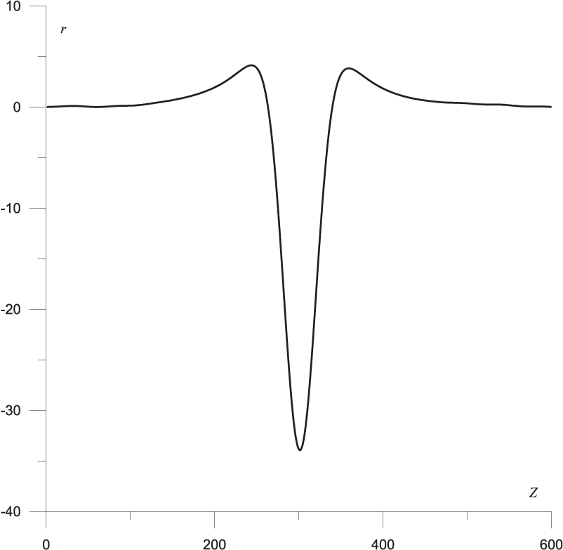
Though amplitude is moderate eigenfunction is similar to eigenfunction of Boussinesq equations.

Calculation here are fulfilled for $R=1$, $\rho=1$, $\mu=1$, $J_{m}=30$, the same values correspond to graphs in sections below; $z_{\infty}^{\prime}=1.1$, $r_{\infty}=1.69$ (small amplitudes), $r_{\infty}=1.55$ (moderate amplitudes).

In order to verify stability of kink solution Riemann problem of arbitrary shock split was solved. Initial data was taken in the step-like form

$$r=r_{01}+(r_{02}-r_{01})\tanh((Z-Z_{0})/L)/2,\quad\dot{r}=0,\quad r_{01}=r_{\infty}$$

$$z^{\prime}=z_{01}^{\prime}+(z_{02}^{\prime}-z_{01}^{\prime})\tanh((Z-Z_{0})/L)/2,\quad\dot{z}=0,\quad z_{01}^{\prime}=z_{\infty}^{\prime}$$

Here $r_{02}$ is some arbitrary value and $z_{02}$ is calculated by formula

$$P_{*}=\frac{\hat{W}_{\lambda_{2}}(r_{02},z_{02}^{\prime})}{r_{02}z_{02}^{\prime}}$$

This formula leads to problem of finding of the root of fifth-order polynomial equation which is solved by Mathematika package. Solution with property $\Delta=z_{02}^{\prime}>z_{01}^{\prime}$ is taken. Note that there is two such solutions. The smaller value is taken below. It means that branch bifurcating from zero for $\Delta=z_{02}^{\prime}-z_{01}^{\prime}$ is used. The higher value leads after some time of evolution to out of correctness calculations. Split into two or three shocks is observed. In the case of three shocks one shock is kink mentioned above. But typically it is travelling kink. Solution with standing kink is found by variation of parameter $r_{02}$. Examples of calculations with positif and negative speed of kink are shown below, fig.9.

Analysis of shock problem solutions and dispersion relation for uniform state of right side from kink shows that line tangent to minus dispersive curve at the origin of coordinates do not intersects it. Dispersion for the origin of coordinates is positive so solitary-wave like shock seen on one of the graphs is predicted by theory. Families of solitary waves of depression tending to kink solution may exist also.

Examples of solutions for the case of large enough initial shock are presented here. In the case of small amplitude no kink is observed. In the case of moderate amplitude uniform state 2 is unstable and calculation of Riemann problem leads to emergency stop.

Now we can analyze another problem essential from the practical point of view. Let we have initial data with two opposite steps:

$$r=r_{02},\quad-d<Z<d;\quad r=r_{01}\quad(-d>Z)\textrm{V}(Z>d)$$

Large scale approach is assumed here, $d$ is some distance. Steps are smoothed in reality. Standing kink solution in this problem corresponds to some critical case. If the speed of left kink is negative then such disturbance will increase it’s area with time and then the speed is positive the area of disturbance will decrease.

The theory of non-dissipative shocks [4]-[12] is applicable for this model and the investigations made above were fulfilled by the aid of methods developed in this theory. This theory is based on analysis of dispersion relation and analysis of dimensions of invariant manifolds of solutions of systems of equations of travelling waves numerical modelling of invariant manifolds and direct calculations of partial equations. So the same structures as in models described in [4]-[12] exists. Extending non-local shocks with solitary wave structure are observed then line $U=\omega/k$ does not intersect dispersive curve and shocks with stochastic structure are observed in the case of intersection.

The equations with controlled pressure are Hamilton equations. But there is no conservation of energy here. Hamiltonian here is not energy. It seems that equations of of travelling waves for this model are non-integrable.

Simplified equations are required to describe centered simple waves. In order to derive simplified equations let’s introduce new notation

$$\quad u=z^{\prime}$$

Now equations takes the form

$$\left(R\hat{W_{1}}\frac{u}{\sqrt{u^{2}+r^{\prime 2}}}\right)^{\prime\prime}-p_{*}(rr^{\prime})^{\prime}=\rho R\ddot{u}$$

$$\left(R\hat{W_{1}}(u,r,r^{\prime})\frac{r^{\prime}}{\sqrt{u^{2}+r^{\prime 2}}}\right)^{\prime}-\hat{W_{2}}(u,r,r^{\prime})+p_{*}ru=\rho R\ddot{r}$$

$$-\hat{W_{2}}(u,r,r^{\prime})+p_{*}ru=0$$

Then let’s take $u$ from second equation and put it to the first equation and withdraw higher order derivatives. Resulting equations takes the form

$$\Phi(r^{\prime\prime},\ddot{r},..\textrm{other.second.order.terms}...;r.\textrm{coefficients.only}.)=0,\ u=\Gamma(r)$$

Here $\Phi$ and $\Gamma$ are some functions.

For moderate values of $\varepsilon$ zones where $\sigma_{1}<0$ appear in the solution. This means according to Petrovski theorem [3] that in this zones equations (3.2) are non-correct. The other problem is that on the boundary of correct and non-correct zone graphs $r(z)$ and $r(Z)$ take the form of broken line. So we have discontinuity of derivative here.

The model formally permits overlapping and breaking but analysis showed that such phenomenons may appear only in the case of compression and hence non-correctness.

One more problem is that there is no dispersion for short waves in this model ($\omega/k\to const$ for $k\to+\infty$). It may cause infinite growth of envelop.

Numerical scheme itself possesses it’s own smoothing and correctional properties so calculation continues some time after non-correct zones appear but later shot-length oscillations arise in non-correct zones and calculation stops due to increase of these oscillations. Numerical solution in non-correct case is usually only approximate solution. Usually there is convergence of numerical scheme in correct case if some stability condition holds and there is no convergence for any choose of relation between time and spatial steps in non-correct case. Hence non-correctness may be revealed numerically also. Petrovskii theorem gives only the necessary condition of correctness so then correctness must be verified numerically.

Obviously non-correctness is related to the fact that membrane model can be used only for the stretched case. Plate model which takes into account bending resistance works in stressed case also. Bending resistance also obviously prevents the plate from braking that is from appearance of discontinuities for $r^{\prime}$. Correction of equations is described in section 7. Note that viscous elasticity model may be used for correction also.

First of all let’s note that the manner of derivation here is differs sufficiently from the manner in which equations (3.2) were derived. Derivation here is based on formulae of linear theory of elasticity and converting of formulae of Euler approach into Lagrange form. The main goal is condemnation of hypothesis made in previous section that implementation of bending resistance may resolve problems appeared in calculations.

Let’s start from well-known Germen-Lagrange formula for stable state of thin unstretched and unstressed plate

$$p_{l}=\frac{Eh^{3}}{12(1-\sigma^{2})}\eta_{xxxx}$$

Here $p_{l}$ is pressure acting on the plate, $\eta$ is vertical displacement, $h$ is horizontal coordinate, $h$ is thickness, $E$ is Yung module, $\sigma$ is Poisson coefficient. Action of internal elastic forces caused by bending of the plate may be replaced by action of corresponding pressure.

For small stretch additional vertical force must be included in left-right side of equations (7)

$$df_{r}=\frac{1}{3}\mu Rr^{\prime\prime\prime\prime}dZ$$

Cylindrical form of surface and incompressibility of material $\sigma=1/2$, $E=3\mu$ are taken into account here.

Equation for $r$ takes the form

$$-cr^{\prime\prime\prime\prime\prime}+\left(R\sigma_{1}\frac{r^{\prime}}{\lambda_{1}^{2}}\right)^{\prime}-\frac{\sigma_{2}}{\lambda_{2}}+p_{*}rz^{\prime}=\rho R\ddot{r}$$

Analysis of dispersion relation shows that now equations are correct independently of whether $\sigma_{1}>0$ or $\sigma_{1}<0$. Calculation with the same parameters as in calculation described in previous section was fulfilled, $c$ was treated as a small parameter. No any problems are found.

Solitary wave splits in the case of correction.

Equations of equations filled by fluid are given below [2]

$$\left(R\sigma_{1}\frac{z^{\prime}}{\lambda_{1}^{2}}\right)^{\prime}-Prr^{\prime}=\rho R\ddot{z},\quad[[-cr^{\prime\prime\prime\prime}]]+\left(R\sigma_{1}\frac{r^{\prime}}{\lambda_{1}^{2}}\right)^{\prime}-\frac{\sigma_{2}}{\lambda_{2}}+Prz^{\prime}=\rho R\ddot{r}$$

$$\dot{r}z^{\prime}-r^{\prime}\dot{z}+vr^{\prime}+\frac{1}{2}rv^{\prime}=0,\quad\rho_{f}(\dot{v}z^{\prime}-v^{\prime}\dot{z}+vv^{\prime})+P^{\prime}=0$$

Here $v$ is fluid velocity, $\rho_{f}$ is fluid density. Correctional term discussed in previous section is included here in double square brackets.

Dispersion relation for these equations was derived in [2]. The main difference from the case of fixed-pressure equations is that both branches intersect in point $\omega=0$, $k=0$.

It is not clear how to calculate these equations. The one way is replace fluid gas by low-compressible gas. The required modification of hydrodynamic part of equations is given below

$$(\dot{\rho_{f}}z^{\prime}-\rho_{f}^{\prime}\dot{z})r^{2}+2\rho_{f}r(\dot{r}z^{\prime}-r^{\prime}\dot{z})+(\rho_{f}vr^{2})^{\prime}=0$$

$$P=P(\rho_{f})$$

Equation of conservation of mass is modified here. Equation of state is added. The problem is wheather dispersion can prevent breaking of waves in gas if $c=0$.

There are three dispersive curves for these equations.

The other way is to eliminate pressure and get three equations

	$\displaystyle\left[\rho_{f}z^{\prime}-\left(\frac{\frac{r^{\prime}\rho R}{rz^{\prime 2}}}{1+\frac{r^{\prime 2}}{z^{\prime 2}}}\right)^{\prime}\right]\dot{v}-\left[\left(\frac{\frac{r^{\prime}\rho R}{rz^{\prime 2}}}{1+\frac{r^{\prime 2}}{z^{\prime 2}}}\right)+\left(\frac{\frac{\rho R}{2z^{\prime 2}}}{1+\frac{r^{\prime 2}}{z^{\prime 2}}}\right)^{\prime}\right]\dot{v}^{\prime}-\left(\frac{\frac{\rho R}{2z^{\prime 2}}}{1+\frac{r^{\prime 2}}{z^{\prime 2}}}\right)\dot{v}^{\prime\prime}=$
	$\displaystyle\rho_{f}(v^{\prime}\dot{z}-vv^{\prime})-[[cr^{\prime\prime\prime\prime}/(rz^{\prime})]^{\prime}]+\quad$
	$\displaystyle\left[\frac{\frac{(1-r^{\prime})\left(R\sigma_{1}\frac{r^{\prime}}{\lambda_{1}^{2}}\right)^{\prime}-\frac{\sigma_{2}}{\lambda_{2}}}{rz^{\prime}}-\frac{\rho R}{rz^{\prime 2}}(\dot{z}-v)\left(\frac{z^{\prime}\dot{z}-vr^{\prime}-\frac{1}{2}rv^{\prime}}{z^{\prime}}\right)^{\prime}-\frac{\rho R}{rz^{\prime 3}}(r^{\prime}\dot{z}-vr^{\prime}-\frac{1}{2}rv^{\prime})(\frac{1}{2}v^{\prime}-\dot{z}^{\prime})}{1+\frac{r^{\prime 2}}{z^{\prime 2}}}\right]^{\prime}$

$$\dot{z}=q$$

$$\rho R\dot{q}=\left(R\sigma_{1}\frac{z^{\prime}}{\lambda_{1}^{2}}\right)^{\prime}-Prr^{\prime}$$

	$\displaystyle P=[[cr^{\prime\prime\prime\prime}/(rz^{\prime})]]+\frac{-1}{1+\frac{r^{\prime 2}}{z^{\prime 2}}}\left[\frac{r^{\prime}\rho R}{rz^{\prime 2}}\dot{v}+\frac{\rho R}{2z^{\prime 2}}\dot{v}^{\prime}\right.$
	$\displaystyle\frac{(1-r^{\prime})\left(R\sigma_{1}\frac{r^{\prime}}{\lambda_{1}^{2}}\right)^{\prime}-\frac{\sigma_{2}}{\lambda_{2}}}{rz^{\prime}}-\frac{\rho R}{rz^{\prime 2}}(\dot{z}-v)\left(\frac{z^{\prime}\dot{z}-vr^{\prime}-\frac{1}{2}rv^{\prime}}{z^{\prime}}\right)^{\prime}$
	$\displaystyle\left.-\frac{\rho R}{rz^{\prime 3}}(r^{\prime}\dot{z}-vr^{\prime}-\frac{1}{2}rv^{\prime})(\frac{1}{2}v^{\prime}-\dot{z}^{\prime})\right]$

These equations are solved by Lax-Wendroff type numerical scheme. Due to combined time-spatial derivatives this scheme is implicit. System of implicit equations is solved by method of iterations. Example of calculation of Riemann problem is given below, fig.10, $v|_{t=0}=0$, $\rho_{f}=1$. Kink and solitary wave-like shocks are clearly seen.

For solitary waves used for shock structures for some given values of physical parameters and phase speed $U$ typically one solution exist. Such one-parametric ($U$ is arbitrary parameter) families of solitary waves in Hamilton systems are typically stable. Here for some special choose of $v$ at infinity these solitary waves may be stationary. There are also other null-parametric stationary solitary waves [11] that are similar to waves investigated for the case of controlled pressure. They exist only for $v=0$. Null-parametric solitary waves in Hamilton systems are typically unstable because if energy of solitary wave is slightly decreased there is no way to return it back. Instability of this waves was verified in [11] by Evans method.

The fluid-filled model is the model with conservation of energy. It leads in the case $c=0$ to integrable system of travelling wave equations and only classical solitary waves and kinks are expected.

Note that the model under consideration due to hydraulic approximation implies slow variation of $r(Z)$ hence simplifications may be fulfilled such that no space-time derivatives will be. But such simplification obviously leads to decrease in accuracy and appearance of non-physical effects. For low-pressure case further simplification may be fulfilled and classical or generalized (if bending resistance is included) Korteweg-de Vries equations may be derived. Detailed analysis of solutions of generalized Korteweg-de Vries equation is fulfilled in [4] and [12]

References

- [1] Fu Y.B., Pearce S.P. Characterization and stability of localized bulging/necking in inflated membrane tubes // IMA J. Appl. Math., 2010. 75, 581-602.
- [2] Fu Y.B., Il’ichev A. Solitary waves in fluid-filled elastic tubes: existence, persistence, and the role of axial displacement // IMA J. Appl. Math., 2010. 75, 257-268.
- [3] Kulikovskii A.G. On the stability of homogeneous states // J. Appl. Math. Mech. 1966. 30. (1). 180-187.
- [4] Bakholdin I. B. Nondissipative shocks in continuum media. Moscow. Fizmatlit. 2004. 318p. In Russian.
- [5]
Bakholdin I.B. Methods of investigation, theory and
classification of
reversible shock structures in models of hydrodynamic type//
Preprins of Keldysh Institute for Applied Mathematics. 2013.
N.30. 40p. In Russian, abstract in English.
URL: http://library.keldysh.ru/preprint.asp?id=2013-30 - [6] Bakholdin I.B. The structure of evolutional jumps in reversible systems // J. Appl. Math. Mech. 1999. V.63. (1). 45-53.
- [7] Bakholdin I.B. Jumps with radiation in models described by the generalized Korteweg-De Vries equation // J. Appl. Math. Mech. 2001. . V. 65. (1). 55-63.
- [8] I. B. Bakholdin and V. Ya. Tomashpol’skii Solitary Waves in the Model of a Predeformed Nonlinear Composite// Differential Equations, 2004, V. 40, N. 4, 571-582.
- [9] Bakholdin I.B. Solitary waves and the structures of discontinuities in non-dissipative models with complex dispersion // J. Appl. Math. Mech. 2003. . V.67. (1). 43-56.
- [10] Bakholdin I. B.and Tomashpol’skii V. Ya. Solitary Waves in the Model of a Predeformed Nonlinear Composite// Differential Equations. 2004. V. 40, N. 4, 571-582
- [11] Ilichev A.T., Fu I.B. Stability of aneurism solutions in fluid-filled elastic membrane tube// Acta Mechanica Sinica. 2012. 28. 1209-1218.
- [12] Bakholdin I.B. Time-invariant and time-varying discontinuity structures for models described by the generalized Korteweg-Burgers equation// J. Appl. Math. Mech. 2011. V. 75 (2), 189-209.