Locally refined discrete velocity grids for stationary rarefied flow simulations
C. Baranger1, J. Claudel1, N. Hérouard1,2, L. Mieussens2
1CEA-CESTA
15 avenue des sablières - CS 60001
33116 Le Barp Cedex, France
(celine.baranger@cea.fr, jean.claudel@cea.fr, nicolas.herouard@cea.fr)
2Univ. Bordeaux, IMB, UMR 5251, F-33400 Talence, France.
CNRS, IMB, UMR 5251, F-33400 Talence, France.
INRIA, F-33400 Talence, France.
(Luc.Mieussens@math.u-bordeaux1.fr)
Abstract: Most of deterministic solvers for rarefied gas dynamics use discrete velocity (or discrete ordinate) approximations of the distribution function on a Cartesian grid. This grid must be sufficiently large and fine to describe the distribution functions at every space position in the computational domain. For 3-dimensional hypersonic flows, like in re-entry problems, this induces much too dense velocity grids that cannot be practically used, for memory storage requirements. In this article, we present an approach to generate automatically a locally refined velocity grid adapted to a given simulation. This grid contains much less points than a standard Cartesian grid and allows us to make realistic 3-dimensional simulations at a reduced cost, with a comparable accuracy.
Keywords: rarefied flow simulation, hypersonic flows, re-entry problem, transition regime, BGK model, discrete velocity model
1 Introduction
The description of a flow surrounding a flying object at hypersonic speed in the rarefied atmosphere (more than 60 km altitude) is still a challenge in the atmospheric Re-Entry community [2]. When this flow is in a rarefied state, that is to say when the Knudsen number (which is the ratio between the mean free path of particle and a characteristic macroscopic length ) is larger than , the flow cannot be accurately described by the compressible Navier-Stokes equations of Gas Dynamics. In this case, the kinetic theory has to be used. The evolution of the molecules of the gas is then described by a mass density distribution in phase space, which is a solution of the Boltzmann equation. In the transitional regime, this equation can be replaced by the simpler Bhatnagar-Gross-Krook (BGK) model.
In order to be able to compute parietal heat flux and aerodynamic coefficients in the range of 60-120 km, a kinetic description of the stationary flow is necessary.
The most popular numerical method to simulate rarefied flows is the Direct Simulation Monte Carlo method (DSMC) [9]. However, it is well known that this method is very expensive in transitional regimes, in particular for flows in the range of altitude we are interested in. The efficiency of DSMC can be improved by using coupling strategies (see [12, 14]) or implicit schemes (see [24, 15]), but these methods are still not very well suited for stationary computations. In contrast, deterministic methods (based on a numerical discretization of the stationary kinetic model) can be more efficient in transitional regimes. Up to our knowledge, there are few deterministic simulation codes specifically designed for steady flows. One of the most advanced ones is the 3D code of Titarev [25] developed for unstructured meshes. Another 3D code has been developed by G. Brook [10]. Other codes exist, but they are rather designed for unsteady problems, see for instance [20, 1] or the recent UGKS scheme developed by K. Xu and his collaborators [27, 18], which is an Asymptotic Preserving scheme for unsteady flows.
In our team, we developed several years ago a code to make 2D plane and axisymmetric simulations of rarefied flows based on the BGK model (see a description in [22, 23, 4]). This code has recently been extended to 3D computations, for polyatomic gases. Due to the physical model (polyatomic gases), the space discretization (block structured mesh), and the parallelization (space domain decomposition with MPI and inner parallelization with openMP), this code is rather different from the other existing 3D codes recently presented in the literature for the same kind of problems (the 3D code of Titarev [25] for example), even if space domain decompositions have already been used for unsteady simulation (see [20]).
All the codes designed for steady flows have a common feature: they are based on a “discrete ordinate” like approach, and use a global velocity grid. This grid is generally a Cartesian grid with a constant step size. The number of points of this grid is roughly proportional to the Mach number of the flow in each direction, and hence can be prohibitively large for hypersonic flows, even with parallel computers. To compute realistic cases (3D configurations with Mach number larger than 20), the velocity space discretization has to be modified in order to decrease CPU time and memory storage requirements. It has already been noticed that a refinement of the grid around small velocities can improve the accuracy and reduce the cost of the computation (especially for large Knudsen numbers in flows close to solid boundaries, see [25]). However, up to our knowledge, there is no general strategy in the literature that helps us to reduce the number of discrete velocities of a velocity grid for any rarefied steady flow, even if some works on adaptive velocity grids have already been presented: the first attempt seems to be [5] for a 1D shock wave problem, and recently, more general adaptive grid techniques designed for unsteady flows have been presented in [21, 13, 19, 11].
The main contribution of this article is to propose an algorithm for an automatic construction of a locally refined velocity grid that allows a dramatic reduction of the number of discrete velocities, with the same accuracy as a standard Cartesian grid. This algorithm uses a compressible Navier-Stokes pre-simulation to obtain a rough estimation of the macroscopic fields of the flow. These fields are used to refine the grid wherever it is necessary by using some indicators of the width of the distribution functions in all the computational domain. This strategy allows us to simulate hypersonic flows that can hardly be simulated by standard methods, since we are indeed able to apply our method to our kinetic code to simulate a re-entry flow at Mach 25 and for temperature and pressure conditions of an altitude of 90 km. In this example, the CPU time and memory storage can be decreased up to a factor 24, as compared to a method with a standard Cartesian velocity grid. Note that preliminary results have already been presented in [6] and [7].
The outline of this article is the following. In section 2, we briefly present the kinetic description of a rarefied gas. In section 3, we discuss the problems induced by the use of a global velocity grid, and our algorithm is presented. Our approach is illustrated in section 4 with several numerical tests. To simplify the reading of the paper, the presentation of our simulation code is made in the appendix.
2 Boltzmann equation and Cartesian velocity grid
2.1 Kinetic description of rarefied gases
In kinetic theory, a monoatomic gas is described by the distribution function defined such that is the mass of molecules that at time are located in an elementary space volume centered in and have a velocity in an elementary volume centered in .
Consequently, the macroscopic quantities as mass density , momentum and total energy are defined as the five first moments of with respect to the velocity variable, namely:
| (1) |
The temperature of the gas is defined by the relation , where is the gas constant defined as the ratio between the Boltzmann constant and the molecular mass of the gas.
When the gas is in a thermodynamical equilibrium state, it is well known that the distribution function is a Gaussian function of , called Maxwellian distribution, that depends only on the macroscopic quantities :
| (2) |
It can easily be checked that satisfies relations (1).
If the gas is not in a thermodynamical equilibrium state, its evolution is described by the following kinetic equation
| (3) |
which means that the total variation of (described by the left-hand side) is due to the collisions between molecules (described by the right-hand side). The most realistic collision model is the Boltzmann operator but it is still very computationally expensive to use. In this paper, we use the simpler BGK model [8, 26]
| (4) |
which models the effect of the collisions as a relaxation of towards the local equilibrium corresponding to the macroscopic quantities defined by (1). The relaxation time is defined as , where is the viscosity of the gas. This definition allows to match the correct viscosity in the Navier-Stokes equations obtained by the Chapman-Enskog expansion. This viscosity is usually supposed to fit the law , where and are reference viscosity and temperature determined experimentally for each gas, as well as the exponent (see a table in [9]).
The interactions of the gas with solid boundaries are described with the diffuse reflection model. Let us suppose that the boundary has a velocity and temperature . In the diffuse reflection model, a molecule that collides with this boundary is supposed to be re-emitted with a temperature equal to , and with a random velocity normally distributed around 0. This reads
| (5) |
if , where is the normal to the wall at point directed into the gas.The parameter is defined so that there is no normal mass flux across the boundary (all the molecules are re-emitted). Namely, that is,
| (6) |
There are other reflection models, like the Maxwell model with partial accomodation, but they are not used in this work.
2.2 Velocity discretization on Cartesian grid
In most of existing computational codes for the Boltzmann equation that use a deterministic method, the velocity variable is discretized with a global Cartesian grid, that is to say the same grid for every point of the space mesh. Consequently, it is necessary to compute a priori a velocity grid in which every distribution function that may appear in the computation can be resolved (see figure 1). This means that the grid must be:
- •
large enough to contain the main part of the distribution functions for every position in the computational domain
- •
fine enough to capture the core of the distribution functions for every position in the computational domain
The corresponding parameters (bounds and step of the grid) can be determined with the following idea: at each point of the computational domain, the macroscopic velocity and temperature give information on the support of the distribution function . Indeed, if is “not too far” from its corresponding Maxwellian, as supposed in the BGK model, its support is centered around , and is essentially localized between bounds that depend on and , corresponding to the standard deviation of the Maxwellian ; that is to say is very small outside (see figure 2 where these bounds are and in 1D). When several distribution functions have to be discretized on the same grid, their supports are reasonably well approximated if the bounds are
| (7) |
and if the grid step is
| (8) |
where is the computational domain (in space), and (see 3). In (7)-(8), the parameters and can be chosen as follows. For , statistical argument suggest that values between and are needed, and so seems to be a good compromise between accuracy and computational cost. The parameter allows us to adjust the grid step: it must be at most equal to 1 (which ensures that there are at least six points inside the core of every distribution function), but a smaller value might be necessary for an accurate computation.
To compute these bounds, it is necessary to a priori estimate the values of and in the computational domain. A simple way is to use a compressible Navier-Stokes (CNS) pre-simulation (for which the CPU time is negligible as compared to the Boltzmann simulation). This simulation gives the fields and in , and the bounds and the grid step can be defined by formulas (7)-(8) applied to these fields, that is to say
| (9) |
and
| (10) |
However, the values of the bounds are mainly determined by the temperatures in the shock zone, which can reach thousands of Kelvin. One must be careful that, at high altitude and high speeds, numerical computations of Navier-Stokes equations can underestimate those temperatures, which would lead to inappropriate bounds.
It is quite clear that the size of the velocity grid increases with the Mach number. Indeed, a large Mach number implies large upstream velocities and large temperature in the shock wave, which lead to very large bounds (see (7)), while the temperature of the body remains small, thus leading to small grid step (see (8)). For realistic re-entry problems, this can lead to prohibitively large grids. For instance, for the flow around a cylinder of radius 0.1 m at Mach 20 and altitude 90 km, formulas (9) and (10) used with a Compressible Navier-Stokes pre-simulation lead to a velocity grid of points and around 350 GB memory requirements with a coarse 3D mesh in space.
However, this is mainly due to the use of a Cartesian grid with a constant step. In order to decrease the size of the grid, it is attractive to refine it only wherever it is necessary, and to coarsen it elsewhere. In the following section, we show that this can be done automatically with our new algorithm.
This approach may not be well designed for cases where is very far from it corresponding Maxwellian (like in shock interactions problem). However, for reentry problems, our assumption is realistic for transitional regime we are interested in.
3 An algorithm to define locally refined discrete velocity grids
Since we have to represent many distribution functions on the same grid, it is natural to refine the grid in the cores of theses distributions, and to coarsen it in the tails (see figure 4). To achieve this goal, we define the concept of “support function”, and we use it to design an AMR (Adaptive Mesh Refinement) velocity grid.
3.1 The support function
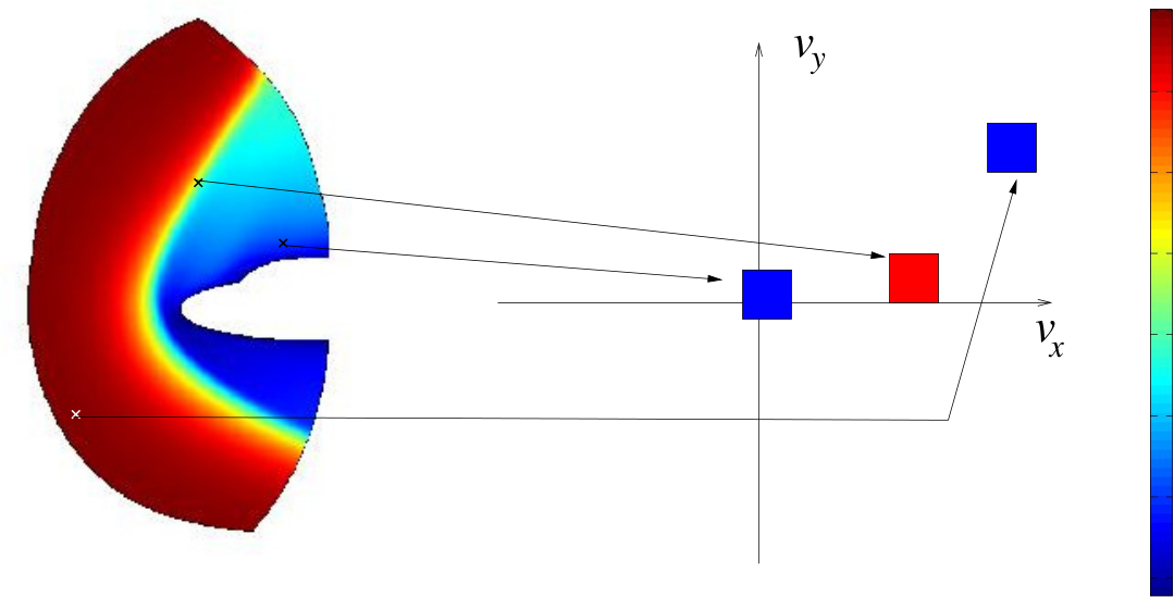
At each point of the computational space domain , and give information on the “main” support of the distribution function in the velocity space: this support is centered at and of size (see (7)). We define the support function in the velocity space as follows: for every in the velocity space, we set if there exists in a such that , that is to say that is inside the support of a distribution, considered as a sphere of center and of radius . This function gives an incomplete mapping of the velocity domain (see figure 5). Now we want to extend this function to the whole velocity space, so that it can be used as a refinement criterion to design an optimal velocity grid.
Indeed, so far, this function is not defined for every , especially for large ones, as we cannot find for every an appropriate pair to match the definition of the support function. Moreover, this function might be multivalued, as there might be two different space points and with same velocity , but with different temperatures . Since our goal is to obtain for every the minimum size of the support of every distribution centered around , these two problems can be avoided as follows :
- (a)
we set if and with . Indeed, the size of the grid around is constrained by the distribution centered on that has the smallest support, hence must have the corresponding smallest possible value.
- (b)
if there is no such that , then is in the tail of every distribution function, and there is no reason to refine the grid there, so we set to its largest possible value .
These ideas lead to the following algorithm for an automatic construction of . Note that below, the computational domain in space is supposed to be discretized with a mesh composed of cells numbered with three indices . This is not a restriction of our algorithm.
Algorithm 3.1 (Construction of the support function).
- 1.
CNS velocity and temperature are stored in arrays and for .
- 2.
- 3.
computation of the field , stored in an descending order in the 1D array , for , so that .
- 4.
initialization of the array on the velocity grid (one value per discrete velocity)
- 5.
(loop on the cells of the space mesh)
-
(loop on the nodes of the velocity grid)
- –
if is in the sphere of center and radius , then it is in the support of a distribution function, and we set
- –
-
This algorithm ensures that the array satisfies the following property.
Property 3.1.
For every between and , we have :
This means that if we take a velocity of the fine grid, then among all the distribution functions whose support contains , one of them has a smallest support, and is the size of its support. This support function hence tells us how the fine Cartesian grid should be refined, or coarsened, around .
The generation of the corresponding adapted grid is described in the following section.
Remark 3.1.
It may happen that with such a strategy, the support function does not take sufficiently into account the support of the wall Maxwellian (for diffuse reflection conditions on a solid obstacle): this Maxwellian is centered around and has a temperature which is often the smallest temperature of the computational domain. This can be the case when the macroscopic CNS flow is not resolved enough close to the wall, or if the CNS equations are solved with slip boundary conditions. In this case, it is safer to add the element in and to add the corresponding velocity in the fine grid.
3.2 AMR grid generation
The idea is to start with a unique cell defined by the bounds of the fine velocity grid (that is the full velocity domain), and then to apply a recursive algorithm: each cell is cut if its dimensions are larger than the minimum of in the cell. The algorithm is the following:
Algorithm 3.2 (Recursive refinement of a cell ).
- 1.
compute the minimum of the field in the cell , that is to say the minimum of the elements of that have the same indices as the discrete velocities of the fine grid included in this cell :
- 2.
if one edge of is larger than , then the cell is cut into 8 new subcells on which the refinement algorithm is applied, recursively.
- 3.
else, the cell is kept as it is, and the cell and its vertices are numbered.
At the end of the algorithm, the final grid satisfies the following property: every cell has a size smaller than the minimum of the support function in the cell.
3.3 An example
We anticipate on the numerical results that will be discussed in section 4 to illustrate the previous algorithms.
The test case is a 2D steady flow around a cylinder at Mach 20 (see the geometry in figure 6 and the physical parameters in section 4.2). A CNS pre-simulation and the use of formula (9)-(10) with parameters and give us a fine velocity grid with points, see figure 7. Algorithms 3.1 and 3.2 applied to the CNS fields give the support function and the AMR velocity grid shown in figure 8. The AMR velocity grid has 529 points, which is one fourth as small as the original fine Cartesian grid.
Note that the AMR grid is refined around the zero velocity and the upstream velocity: these velocities correspond to the flow close to the solid boundary and to the upstream boundary, where the temperature is low, thus where the distribution functions are narrow, and hence where, indeed, we need a fine velocity resolution. At the contrary, the grid is coarse close to its boundaries: the discrete velocities are very large there and are all in the tails of all the distribution functions, where, indeed, we do not need a fine resolution.
The accuracy of the computation on this AMR grid is studied in section 4.
3.4 Discrete Velocity Approximation on the AMR velocity grid
When one wants to transform a standard discrete velocity method based on a Cartesian grid to a method using our AMR grid, two points have to be treated carefully: the computation of the moments of , and the approximation of the collision operator. In this paper, we only use the BGK collision model of the Boltzmann equation: therefore its approximation (based on the conservative approach of [23]) reduces to the problem of a correct approximation of the moments of , as it is described below.
First note that the standard discrete velocity approach consists in replacing the kinetic equation (3) by the following discrete kinetic equation
| (11) |
where is supposed to be an approximation of for every discrete velocity , with to . The discrete distribution function is , and is the discrete collision operator. The moments of the discrete distribution function are obtained by using a quadrature formula to replace (1) by
where are the weights of the quadrature.
For the BGK model (4), the conservative approximation of [23] gives the following discrete BGK collision operator
where is the discrete Maxwellian that has the same discrete moments as . It can be shown that there exists such that , that is to say, is the unique solution of the nonlinear system
where we note . This system can be solved by a Newton algorithm (see details in [23] and a more economic version of the algorithm due to Titarev in [25]).
Consequently, to apply this approach to our AMR velocity grid, we just have to chose a quadrature formula. First, we propose the standard bilinear interpolation of on each cell of the AMR grid (by using the four corners of the cell). In this case, the quadrature points are the nodes of the grid, and so are the discrete velocities that are used in the transport term. The quadrature weights are
where in 3D or in 2D, and is the volume (or the area in 2D) of .
The number of discrete velocities can be decreased if we take a simpler (constant per cell) interpolation. Here, the quadrature points are the centers of the cells, and so are the discrete velocities that are used in the transport term. The weights are simply the volume (or the area) of the cells: . Note that the number of discrete velocities that are used with this approach is equal to the number of cells of the AMR grid, which is smaller than the number of nodes, see section 4.2. We advocate the use of this latter approach, since it allows to save a lot of computer memory, and since we observed with our tests that the interpolation does not give more accurate results.
Remark 3.2.
Our AMR velocity grids are often very coarse at their boundaries (since velocities are very large there, and are in the tails of all the distribution functions). Consequently, passing from to a grid may lead to a grid which is not large enough. Indeed, if the grid is of length (in the direction, for instance) and its outer cells are of length , then the length of the grid now is . If is large, the grid is not large enough. In that case, it is thus safer to modify step 2 of Algorithm 3.1 by increasing the bounds of the fine Cartesian grid: and are replaced by and for example, where is the step of the fine grid.
3.5 AMR grid generation for axisymmetric flows
Many interesting 3D flows have symmetry axis (like flows around axisymmetric bodies with no incidence). In that case, if we assume that the symmetry axis is aligned with the coordinate, it is interesting to write the kinetic equation in the cylindrical coordinate system , since the distribution function is independent of , and we get
| (12) |
where and are the cylindrical coordinates of the velocity in the local frame , that is to say and .
If the velocities of the upstream flow and of the solid boundaries have no component in the direction, then is even with respect to . Indeed, using the Galilean invariance of equation (12), we apply the symmetry with respect to the plane to the equation to get that is also a solution.
In this case, the discrete velocity grid must be constructed for variables , where is non negative, is in , and can take any value. The construction of this grid is slightly different from the Cartesian case. We briefly comment on these differences in this section.
First, bounds in and directions can be easily obtained and we set
| (13) | ||||||
where and are the macroscopic velocities in the axial and radial directions. Since is a bounded variable, there is nothing else to do at this level.
The steps and of the initial grid are obtained by (10) for and . However, the choice of the step in the direction is not obvious. Indeed, this variable has no link with the width of the distribution. Moreover, the grid in this direction must be fine enough to capture the derivative , while in the other directions, only some moments have to be captured. After several tests (and from the experience made in [23]), it seems that a grid step such that there are 30 points uniformly distributed in is a good compromise between cost and accuracy.
To refine/coarsen this initial cylindrical grid, we choose to use the procedure described in the steps of sections 3.1 and 3.2 in the plane to generate a two-dimensional AMR grid. Indeed, for the same reasons as mentioned above, there is no reason to refine or coarsen the grid in the direction. Then, the complete grid is obtained by a rotation of the two-dimensional AMR grid in the direction, with the same step as in the initial grid. This procedure is simple and turned out to be very efficient.
4 Numerical results
4.1 The 3D kinetic code
Our 3D kinetic code is written in Fortran, and can deal with 2D planar flows, or 2D axi-symmetric flows as well as 3D flows on multiblock curvilinear structured grids. A steady state solution of the BGK equation for monoatomic or polyatomic gases is computed with a linearized implicit finite volume scheme, based on a velocity discretization which is conservative and entropic (see [22]). In axisymmetric cases, a specific scheme (named T-UCE) is used in order to ensure a conservative and entropic discretization of the transport operator (see [23]).
In order to deal with high computational costs (in 3D configurations for example), an hybrid parallel implementation is used: a domain decomposition in the position space used with the library routines specified by the Message Passing Interface (MPI) can deal with a large number of mesh cells. Note that this is the opposite of the strategy used in [25] (which uses a domain decomposition in the velocity space). Moreover, the OpenMP library is used with 8 threads for loops computations that are local w.r.t the position (computation of the moments, Maxwellian, etc.), thus large numbers of velocity points can be reached. We also use OpenMP for loops that are local w.r.t the velocity, like the computation of the transport terms, for instance. The communication between different domains are treated as explicit boundary conditions. This code has been run on the super-computer TERA-100 of the CEA (that has around cores Intel Xeon 7500), by using at most 1600 cores.
Since a general description of our code is not the main subject of this paper, we do not give more details here. However, for completeness, note that interested readers can find a more detailed description of the code in the appendix.
The distribution is initialized by using a CNS pre-simulation (also used for the AMR strategy): the number of iterations before reaching convergence is then considerably decreased (see section 4.5).
For the 2D plane examples shown below, we use a simpler version of the code, called CORBIS. This code is based on the same tools but makes use of the reduced distribution technique to reduce the velocity space to 2D only. This code only uses OpenMP directives to work on parallel computers (see [4]). It has been used on a SMP node of 48 cores AMD-Opteron-8439-SE.
For the compressible Navier-Stokes simulations, we use a 3D code developed by the CEA-CESTA for hypersonic flows at moderate to low altitudes. The same techniques as in our 3D kinetic code are used: a finite volume linearized implicit scheme with multiblock structured meshes. On solid walls, no-slip and isothermal boundary condition are used ( and ).
4.2 A 2D plane example
Here, we illustrate our approach with the simulation of a steady flow over a infinite cylinder of radius m at Mach 20, for density and pressure of the air at an altitude of 90 km. The gas considered here is argon (molecular mass). Namely, we have , , and . The temperature of the wall is . The downstream flow is ignored, and outflow boundary conditions are used at the boundary of the right side of the domain. Since the flow is invariant along , the simulation is made with the 2D plane model in the plane . Finally, since the flow is symmetric with respect to the line , the computation is made on the upper part on this plane only (see figure 6). See appendix A.2 for the implementation of the boundary conditions in the code.
The space mesh uses cells, with a refinement such that the first cell at the solid boundary is smaller than one fifth of the mean free path at the boundary.
A CNS pre-simulation and the use of formula (9-10) with parameters and give us a fine velocity grid with points (bounds and for and with a step of , in m.s-1), see figure 7. Algorithms 3.1 and 3.2 applied to the CNS fields give the support function and the AMR velocity grid shown in figure 8. The AMR velocity grid has 529 points, which is one fourth as small as the original fine Cartesian grid. This gain can be further increased if we define the discrete velocities as the centers of the cells of the AMR grid rather than its vertices. This gives 316 discrete velocities, hence with a gain of 6.7 times instead of 4.
First, we compare the CPU time required by the code CORBIS with the different velocity grids. While the number of iterations to reach steady state is approximately the same with both grids, the CPU time required by the original fine Cartesian velocity grid is around 7 times as large as with the new AMR grid, which is almost the same ratio as the ratio of the number of discrete velocities. The memory required with the uniform grid method is around 170 MB whereas with the use of the AMR grid, only 25 MB of memory storage is required. This shows that the new AMR grid leads to a real gain both in memory storage and CPU time.
Then, we compare the accuracy of the results with the two grids for the macroscopic quantities. We compute the normal component of the heat flux to the boundary, which is a quantity of paramount importance in aerodynamic simulations: we find a maximum relative difference lower than 5%, which is reasonably small (see the profile of this flux on figure 9). We also compute the differences for the density, temperature and pressure in the whole computational domain:
- •
the mean quadratic relative difference over all the cells of the computational domain is 5% for the density, 1% for the temperature, 0.6% for the horizontal velocity, and 1.2% for the vertical velocity;
- •
the maximum relative difference on each cell of the computational domain is 40% for the density, 69% for the temperature, and 157% for the velocity.
The maximum relative differences are observed at the solid wall for the density and the velocity, and in the upstream flow for the temperature.
This difference is quite large, and can be explained as follows. The smallest cells of our AMR velocity grid (that are around small velocities, like velocities at the solid wall) turn out to be smaller than the cells of the Cartesian grid (size instead of ). This means that our results with the AMR grid are probably more accurate than the results of the Cartesian grid. Consequently, the Cartesian grid results should not be considered as a reference for this comparison.
To confirm this analysis, we make a new simulation with a Cartesian grid with a uniform step of (like the smallest step of the AMR grid). We observe that relative differences between the Cartesian grid and the AMR grid are much smaller:
- •
the mean quadratic relative difference over all the cells of the computational domain is 2% for the density, 0.5% for the temperature, 0.3% for the horizontal velocity, and 0.7% for the vertical velocity;
- •
the maximum relative difference on each cell of the computational domain is 12% for the density, 13% for the temperature, 80% for the velocity.
The maximum relative difference is still too large for the velocity (80% at the boundary), but this quantity is very small in this zone and probably requires smaller velocity cells (that is a smaller parameter for both grids). However, this inaccuracy does not deteriorates the results on the other quantities, in particular for the heat flux at the boundary. Indeed, the comparison of the heat fluxes is even better, since we find a relative difference lower than 2.5%, which is excellent. The comparison in terms of CPU time and memory storage is of course more favorable to the AMR grid here.
Note that we also did the same computations with an finer AMR grid obtained with the parameter : the difference with is less than 2% for the heat flux at the solid wall, which is quite good. The value is then clearly sufficient. However, if one is interested with the flow velocity at the boundary, we advocate to use , since the differences here are around 15%.
4.3 A 2D axisymmetric example
Here we consider the flow around a sphere of radius 0.1 m, at Mach 20, for density and pressure of the air at an altitude of 90 km (see figure 10).The gas is air (molecular mass kg), considered as a diatomic gas. Namely, the upstream density and pressures are , and , and the temperature of the surface of the sphere is . The downstream flow is ignored, and outflow boundary conditions are used at the boundary of the right side of the domain. Since the flow is rotationally symmetric, the simulation is made with the 2D axisymmetric model in the plane . Finally, since the flow is symmetric with respect to the line , the computation is made on the upper part on this plane only.
The space mesh uses cells, with a refinement such that the first cell at the solid boundary is smaller than one fifth of the mean free path at the boundary. A CNS pre-simulation and the use of formula (13) with parameter give us the following velocity bounds and for , 0 and for , and the bounds for are always 0 and , as explained in section 3.5.
All the following simulations were made with 140 domains and 4 OpenMP threads per domain.
First, a fine uniform cylindrical velocity grid is obtained with (10) and : this gives discrete velocities. The steady state is reached after iterations, in . The corresponding temperature and velocity fields are shown in figure 11.
Then a cylindrical AMR grid is generated (with ): it gives discrete velocities (with the points), the steady state is reached after iterations, in . The support function and AMR grid are shown in figure 12. Here, the gain factors in memory and in CPU time with respect to the uniform grid are around 9.
Now, we use the same AMR grid, but with the points (that is to say the centers of the cells), which gives discrete velocities only. The number of iterations is close (), and the CPU time is . Here, the gain factors in memory and CPU time, with respect to the uniform grid, are around 10.
Finally, we compare in figure 13 the normal heat flux at the boundary for the uniform grid and the AMR grid generated by using the CNS fields ( version). As in the 2D example, we find that the fluxes are very close (with a relative difference which is less than 1%). We get the same results with the version.
Consequently, the AMR grid ( version) is the most efficient here: it gives the same results as the fine uniform grid, for computational and memory cost which is one ninth as small.
Remark 4.1.
Before discussing a full 3D case, we briefly mention another experiment we have done here. We have tried to see if the use of a CNS pre-simulation could be avoided by using a direct estimation of the extreme values of the velocity and the temperature given by the Rankine-Hugoniot relations. Indeed, before the computation, we know the upstream values and , and we can compute the downstream values by the Rankine-Hugoniot relations for a stationary shock. Then we have three set of different values: upstream, downstream, and wall values , and we can use these three sets in our algorithm 3.1 instead of the CNS fields .
With the same test case, this strategy gives a grid with points only (with ), which is half as less as with the CNS fields. The support function and AMR grid are shown in figure 14: of course, since we only have three values for the macroscopic fields here, the grid is not as smooth as with the CNS fields.
Moreover, the convergence to steady state is much slower (since we cannot use the CNS solution as an initial state, see section 4.5 for a comment on the initialization). More important, the accuracy observed on the heat flux is not as good as with the CNS fields: the difference with the fine uniform grid is here around 8% instead of 1%.
Consequently, even if strategy is simple and does not require a CNS solver, it seems to be not accurate enough.
4.4 A 3D example
Here, we consider the flow around a 3D object composed of cone with a spherical nose, with no incidence (see figure 15). The physical parameters are the same as in section 4.3. The space mesh uses cells, with 50 in the direction normal to the surface. Again, the downstream flow is ignored, and outflow boundary conditions are used at the boundary of the right side of the domain.
A CNS pre-simulation and the use of formula (13) with parameter and give us a uniform Cartesian grid with discrete velocities. This is much too large to make the simulation (the memory storage itself is huge). Then we only do the simulation with the AMR grid ( version) generated by our algorithm which has only points.
The gain factor in memory storage is 22. The steady state is reached in iterations and with 400 domains and 4 threads per domain.
To estimate the gain in CPU that would be obtained if the uniform Cartesian grid could be used, we use the following remark: on the previous tests (2D plane and axisymmetric), the number of iterations to reach the steady state is almost the same for the uniform and the AMR velocity grids. Then we make a single iteration with the uniform Cartesian grid (same domain decomposition) and we multiply the CPU time obtained for this iteration by the number of iterations required with the AMR grid. We find a CPU time which is 24 times as large as with the AMR grid, which is quite important. This CPU gain is larger that the gain observed for the memory storage.
4.5 Initialization with the CNS results
Since we use a CNS pre-simulation to build our discrete velocity grid, it is interesting to use it also to initialize the BGK computation, what was done in the previous simulations. It helps to reach the steady state more rapidly, as it is shown in the following example.
We take the same test case as in section 4.3, with the uniform velocity grid. In a first computation, the distribution is initialized with the (Maxwellian) upstream flow (this is the standard initialization), and the scheme converges to the steady state in iterations. Then we do the same computation, but now the initial state is the Maxwellian distribution computed with the macroscopic variables that are given by the steady CNS solution. Then the steady state is reached in iterations only.
A similar gain (half as many iterations as with the standard initialization) is obtained in all our test cases.
5 Conclusion and perspectives
In this paper, we have proposed a method to refine and coarsen a global velocity grid of a discrete velocity approximation of a kinetic equation. It is based on a criterion called “the support function” that links the local size of the velocity grid to the macroscopic temperature an velocity of the flow. Our algorithm uses the macroscopic fields given by a compressible Navier-Stokes pre-simulation to automatically generates an optimal velocity grid.
This approach has been tested in a 3D computational code (and 2D plane and axisymmetric versions) which uses the BGK model of rarefied gas dynamics. Typical test cases in hypersonic re-entry problems (for simplified geometries) have been used. We observed that using our algorithm allows important gains both in CPU time and memory storage, up to a factor 24. This allows to make simulations that are hardly possible with standard grids, even on super computers.
Note that this work might be extended to unsteady flow simulations: we could indeed modify the velocity grid at different time steps according to our refinement algorithm. This might also be used during the iterations of our iterative solver for a steady simulation. However, this would require to interpolate the solution between two successive grids, and this might lead to an important increase of the CPU time. This clearly requires more investigations to get an efficient method.
An obvious, and straightforward, extension of this work will be the use of modified BGK models (like ES or Shakhov models), in order to have a model with a correct Prandtl number.
Moreover, we will try to investigate non isotropic AMR velocity grids by taking into account translational kinetic temperatures in different directions, that can be obtained by the stress tensor computed by the CNS simulation. It could also be interesting to refine the grid so as to capture the discontinuity of the distribution function in the velocity space, but this will require a rather different approach.
Our main short term project is to improve the physical accuracy of our code by implementing a simple BGK-like model for multi-species reactive flows. An application of our method to the full Boltzmann collision operator is less obvious but might also be explored.
Acknowledgment.
Experiments presented in this paper were carried out using the PLAFRIM experimental testbed, being developed under the Inria PlaFRIM development action with support from LABRI and IMB and other entities: Conseil Régional d’Aquitaine, FeDER, Université de Bordeaux and CNRS (see https://plafrim.bordeaux.inria.fr/).
References
- [1] A. Alexeenko and S. Chigullapalli. Unsteady 3d rarefied flow solver based on boltzmann-esbgk model kinetic equations. In 41st AIAA Fluid Dynamics Conference, 2011.
- [2] J. Anderson. Hypersonic and High-Temperature Gas Dynamics, Second Edition. AIAA Education Series. American Institute of Aeronautics and Astronautics, 2006.
- [3] P. Andriès, P. Le Tallec, J.-F. Perlat, and B. Perthame. The Gaussian-BGK model of Boltzmann equation with small Prandtl number. Eur. J. Mech. B/Fluids, 2000.
- [4] K. Aoki, P. Degond, and L. Mieussens. Numerical simulations of rarefied gases in curved channels: thermal creep, circulating flow, and pumping effect. Commun. Comput. Phys., 6:919–954, 2009.
- [5] V.V. Aristov. Method of adaptative meshes in velocity space for the intense shock wave problem. USSR J. Comput. Math. Math. Phys., 17(4):261–267, 1977.
- [6] C. Baranger, J. Claudel, N. Hérouard, and L. Mieussens. Deterministic rarefied flow simulation using non cartesian velocity grids. In ICIAM 2011, Vancouver, Canada, 2011. Minisymposium ”Advanced Numerical Methods for Kinetic Simulations and Their Applications”.
- [7] C. Baranger, J. Claudel, N. Hérouard, and L. Mieussens. Locally refined discrete velocity grids for deterministic rarefied flow simulations. AIP Conference Proceedings, 1501(1):389–396, 2012.
- [8] P.L. Bhatnagar, E.P. Gross, and M. Krook. A model for collision processes in gases. I. small amplitude processes in charged and neutral one-component systems. Phys. Rev., 94:511–525, 1954.
- [9] G.A. Bird. Molecular Gas Dynamics and the Direct Simulation of Gas Flows. Oxford Science Publications, 1994.
- [10] R. G. Brook. A parallel, matrix-free newton method for solving approximate boltzmann equations on unstructured topologies. PhD thesis, The University of Tennessee at Chattanooga, 2008.
- [11] S. Brull and L. Mieussens. Local discrete velocity grids for deterministic rarefied flow simulations. submitted.
- [12] J. M. Burt and I. D. Boyd. A hybrid particle approach for continuum and rarefied flow simulation. Journal of Computational Physics, 228:460–475, 2009.
- [13] S. Chen, K. Xu, C. Lee, and Q. Cai. A unified gas kinetic scheme with moving mesh and velocity space adaptation. Journal of Computational Physics, 231(20):6643 – 6664, 2012.
- [14] P. Degond and G. Dimarco. Fluid simulations with localized boltzmann upscaling by direct simulation Monte-Carlo. J. Comput. Phys., 231(6):2414–2437, 2012.
- [15] G. Dimarco and L. Pareschi. Hybrid multiscale methods. II. Kinetic equations. Multiscale Model. Simul., 6(4):1169–1197, 2008.
- [16] B. Dubroca and L. Mieussens. A conservative and entropic discrete-velocity model for rarefied polyatomic gases. In CEMRACS 1999 (Orsay), volume 10 of ESAIM Proc., pages 127–139 (electronic). Soc. Math. Appl. Indust., Paris, 1999.
- [17] A. B. Huang and D. L. Hartley. Nonlinear rarefied couette flow with heat transfer. Phys. Fluids, 11(6):1321, 1968.
- [18] J.C. Huang, K. Xu, and P.B. Yu. A unified gas-kinetic scheme for continuum and rarefied flows ii: Multi-dimensional cases. Communications in Computational Physics, 3(3):662–690, 2012.
- [19] V.I. Kolobov and R.R. Arslanbekov. Towards adaptive kinetic-fluid simulations of weakly ionized plasmas. Journal of Computational Physics, 231(3):839 – 869, 2012.
- [20] V.I. Kolobov, R.R. Arslanbekov, V.V. Aristov, A.A. Frolova, and S.A. Zabelok. Unified solver for rarefied and continuum flows with adaptive mesh and algorithm refinement. Journal of Computational Physics, 223(2):589 – 608, 2007.
- [21] V.I. Kolobov, R.R. Arslanbekov, and A.A. Frolova. Boltzmann solver with adaptive mesh in velocity space. In 27th International Symposium on Rarefied Gas Dynamics, volume 133 of AIP Conf. Proc., pages 928–933. AIP, 2011.
- [22] L. Mieussens. Discrete Velocity Model and Implicit Scheme for the BGK Equation of Rarefied Gas Dynamics. Math. Models and Meth. in Appl. Sci., 8(10):1121–1149, 2000.
- [23] L. Mieussens. Discrete-velocity models and numerical schemes for the Boltzmann-BGK equation in plane and axisymmetric geometries. J. Comput. Phys., 162:429–466, 2000.
- [24] L. Pareschi and G. Russo. Time relaxed Monte Carlo methods for the Boltzmann equation. SIAM J. Sci. Comput., 23(4):1253–1273 (electronic), 2001.
- [25] V. A. Titarev. Efficient deterministic modelling of three-dimensional rarefied gas flows. Communications in Computational Physics, 12(1):162–192, 2012.
- [26] P. Welander. On the temperature jump in a rarefied gas. Arkiv für Fysik, 7(44):507–553, 1954.
- [27] K. Xu and J.-C. Huang. A unified gas-kinetic scheme for continuum and rarefied flows. J. Comput. Phys., 229:7747–7764, 2010.
- [28] H. C. Yee. A Class of High-Resolution Explicit and Implicit Shock-Capturing Methods. Von Karman Institute for Fluid Dynamics, Lectures Series, no4. Von Karman Institute for Fluid Dynamics, 1989.
Appendix A Overview of the 3D kinetic code
A.1 The linearized implicit scheme
Our code is an extension of the code presented in [23] to 3D polyatomic flows. It is based on the following reduced BGK model
where is the vector of macroscopic mass, momentum, and energy density. Here, we use the standard notation for any vector valued function of , is the vector of collisional invariants, and . Moreover, is the standard Maxwellian distribution defined through the density, velocity, and temperature corresponding to the vector above (see (2)).
This model comes from the reduction of a BGK model for the full distribution function , where is the internal energy variable, and is the number of internal degrees of freedom (see [17] for the first use of this technique and [3] for an application to polyatomic gases). Consequently, it accounts for any number of internal degrees of freedom. For instance, a diatomic gas can be described with .
This model is first discretized with respect to the velocity variable. We follow the approximation of [23] and its extension to polyatomic gases [16]. We assume we have a velocity grid (like the grids described in this paper). The continuous distributions and are then replaced by their approximations at each point , and we get the following discrete velocity BGK system
where is an approximation of that has to be defined. As explained in this paper, we assume we have quadrature weights corresponding to our discrete velocity grid, so that the moment vector of the discrete distributions is
As proposed in [16], the discrete equilibrium is constructed so that it has the same moments as , that is to say
| (14) |
In our code, is determined through the entropic variable such that and , by solving (14) by a Newton algorithm. We mention that the computational cost of this algorithm can be significantly reduced by using a nice idea due to Titarev [25]. This optimization will be used in a future version of our code.
The discrete velocity BGK system is then discretized by a finite volume scheme on a multiblock curvilinear 3D mesh of hexahedral cells , with indices to , respectively. Denoting by an approximation of the average of at time on a cell at the discrete velocity , our scheme reads, in its implicit version,
where
The discrete divergence is given by the following second order upwind approximation (with the Yee limiter [28]):
| (15) |
where
is the second order numerical flux across the face between and , and is the normal vector to this face directed from to while its norm is equal to the area of the face. In the minmod limiter function, we use the notation . Finally, we use the standard notation for every number . The numerical fluxes across the other faces are defined accordingly. For the sequel, it is useful to denote by the corresponding linear first order upwind discretization (that is to say, defined by (15) where the minmod term is set to 0).
The advantage of the time implicit approximation is that it ensures unconditional stability, which allows us to take large time steps, and hence to get rapid convergence to the steady state. Of course, this scheme is too expensive, since it requires to solve a non linear system at each time iteration. Therefore, we rather use the following linearization. First, the Maxwellian is linearized by a first order Taylor expansion:
and the same for (see section A.4 for explicit expressions of the Jacobian matrices). Then the discrete divergence, which is not differentiable due to the limiter, is linearized by using the corresponding first order upwind approximation. This is sometimes called a “frozen coefficient technique”, which gives
Then, denoting by (same notation for ), and by the moments of , our scheme reads in the following form:
| (16) | ||||
| (17) |
where the right-hand sides are given by
If our scheme converges to steady state, then the right-hand side is zero, and we get a second order discrete steady solution.
A.2 Numerical boundary conditions
Numerically, the boundary conditions are implemented by the standard ghost cell technique, which is used as follows. When an index corresponds to a cell located at the boundaries of the domain, there appear unknown values in the numerical fluxes like and , for the cells and for instance (see (15)). Corresponding cells , , etc. are called ghost-cells. These values are classically defined according to the boundary conditions that are specified for the problem. Here we use several kinds of boundary conditions: solid wall interactions, inflow and outflow boundary conditions at artificial boundaries, as well as symmetry boundary conditions along symmetry planes and symmetry axes.
For the diffuse reflection, the incident molecules in a boundary cell of index are supposed to be re-emitted by the wall from a ghost cell of index . This cell is the mirror cell of with respect to the wall. The diffuse reflection (5)–(6) is then modeled by
| (18) |
where is determined so as to avoid a mass flux across the wall, that is to say between cells and . In this relation, is a discrete conservative approximation of the wall Maxwellians . Relation (6) gives
For the inflow boundary condition, for instance at a boundary cell , we simply set the ghost cell value to the upstream Maxwellian distributions (defined through the upstream values of , , and ):
For the outflow boundary condition, we set the ghost cell value to the value of the corresponding boundary cell:
Finally, for a cell in a symmetry plane (for instance the plane ) we use the symmetry of the distribution functions to set
where is such that is the symmetric of with respect to the symmetry plane. In this case, our AMR velocity grid is constructed such that it is also symmetric with respect to this plane, which gives . This grid is obtained in two steps: first, a part on one side of the symmetry plane is obtained by using our algorithms (support function and AMR grid generation), and then this part is symmetrized to obtain the part on the other side.
For the second order numerical flux, we also need the values of a second layer of ghost cells with indices like or , etc. For these values, we simply copy the value of the corresponding ghost cell in the first layer, that is to say for instance. This treatment makes the accuracy of our scheme reduce to first order at the boundary (since this makes the flux limiters equal to 0). It may be more relevant to use extrapolation techniques, which is the subject of a work in progress. Only the boundary condition on a symmetry plane is treated differently: here, we use the symmetry of the distributions to set
where has been defined above.
A.3 Linear solver
At each time iteration, our linearized implicit scheme requires to solve the large linear system (16–17). It is therefore interesting to write it in the following matrix form:
where is a large vector that stores all the unknowns, is the unit matrix, is a matrix such that
| (19) |
is the relaxation matrix such that
| (20) |
and .
For simplicity, we use explicit boundary conditions, which means in ghost cells. This implies that has a simple block structure, which is used in the following.
The algorithm used in our code is based on a coupling between the iterative Jacobi and Gauss-Seidel methods. First, the relaxation matrix is splitted into its diagonal and its off-diagonal , so that we get the following system (this the Jacobi iteration):
| (21) |
Note that is very sparse: the product is local in space and can be written (see section A.4). The left-hand side of this system has a three level tridiagonal block structure. We solve it by using a line Gauss-Seidel iteration which is described below.
With curvilinear grids, in many cases, and in particular for re-entry problems, the flow is aligned with a mesh (generally aligned with solid boundaries), which means that the largest variations occur along the orthogonal direction, say the direction of index , for instance. The idea is to use an “exact” inversion of along this direction. This is done with a sweeping strategy sometimes called “Gauss-Seidel line iteration”. First, we rewrite system (21) pointwise, as follows:
where coefficients are standard notations
for line-Gauss-Seidel method and can be easily derived
from (21), (19),
and (15). Then the linear solver reads as shown in
Algorithm 1.
Remark A.1.
- 1.
We observe that we get a fast convergence to steady state by using a few step of this linear solver (say or 3). This is due to the “exact” inversion along the direction of largest variation of the flow.
- 2.
In practice, we add one back substitution step right after each forward substitution step.
- 3.
This solver is a straightforward extension of the linear solver used in [23]. More sophisticated versions of this solver could be tested.
A.4 Jacobian matrices and the relaxation matrix
Elementary calculus gives the following formula:
where is the following matrix
Consequently, by using the definition (20) of the relaxation matrix , a careful algebra shows that its diagonal elements can be separated into the following two blocks :
Therefore, the product of the off-diagonal part of with (as used in algorithm 1) is simply




.


