Distributional Ergodicity in Stored-Energy-Driven Lévy Flights

Single particle tracking experiments in biological systems often show that diffusion is not normal but rather anomalous [1, 2, 3, 4, 5, 6]; that is, the mean square displacement (MSD) does not grow linearly with time but follows a power-law scaling

Because anomalous diffusions including subdiffusion ($\beta<1$) as well as superdiffusion ($\beta>1$) are ubiquitously observed in many biological experiments, anomalous diffusion is believed to play significant roles in cell biology such as gene regulation [7] and active transports [1, 6]. However, the underlying physical mechanisms remain controversial.

To understand the underlying mechanisms of these anomalous diffusions, phenomenological models such as continuous-time random walk (CTRW), Lévy walk and flight, and other stochastic models of anomalous diffusion have been intensively studied [8, 9, 10, 11, 5, 12, 13]. Among these models, CTRW shows a prominent feature called distributional ergodicity [10, 11, 12, 14]; that is, the time average of an observable converges to a random variable, i.e., convergence in distribution, but it does not coincide with the ensemble average as in the ordinary sense of ergodicity. It is considered that this distributional behavior of time-averaged observables in CTRW is related to large fluctuations of transport coefficients in single particle tracking experiments [2, 3, 4, 5]. It is known that such distributional behavior is universal in infinite ergodic theory [15, 16], where ergodicity is satisfied with respect to an infinite (non-normalizable) invariant measure. This is a completely different feature from other stochastic models of subdiffusion.

While uncoupled CTRWs, in which trapping time and jump length are mutually independent, are extensively studied, effects of a coupling between them become physically important for nonthermal systems such as cells [1, 6]. In such nonthermal systems, a particle in a trapped state would not be simply frozen, but rather it would be storing a sort of energy for the next jump. Thus, a random walk driven by an stored energy during a trapped state is essential in such nonthermal systems, and it will also be important in complex systems such

as finance [17] and earthquakes [18].

As a prototype model of such nonthermal random walks, we study a CTRW with jump lengths correlated with trapping times [19, 20, 21], which we refer to as the stored-energy-driven Lévy flight (SEDLF). The SEDLF exhibits a whole spectrum of diffusion: sub-, normal-, and super-diffusion, depending on a parameter $\gamma$, which characterizes the coupling strength between jump length and trapping time. Here, we show a novel type of distributional ergodicity. In particular, time-averaged observables such as the time-averaged MSDs (TAMSDs) are intrinsically random even when the measurement time goes to infinity.

The SEDLF is based on CTRW with a non-separable joint probability of trapping time and jump length. In general, CTRW is defined through the joint probability density function (PDF) $\psi(x,t)$, where $\psi(x,t)dxdt$ is the probability that a random walker jumps with length $[x,x+dx)$ just after it is trapped for period $[t,t+dt)$ since its previous jump [22, 23]. In particular, the separable case $\psi(x,t)=w(t)l(x)$, in which the jump length and the trapping time are mutually independent, has been extensively studied [24, 8, 10, 11, 12]. Here, we consider a non-separable case defined by

where $w(t)$ is the PDF of trapping times and $\gamma\in[0,1]$ is a coupling strength. Note that a random walker undergoes a long trapped state before it performs a long jump (Fig. 1). In addition, we assume that the PDF of trapping times follows a power law:

as $t\to\infty$. Here, $\alpha\in(0,1)$ is the stable index, a constant $c_{0}$ is defined by $c_{0}={c}/{|\Gamma(-\alpha)|}$ with a scale factor $c$.

For $\gamma=0$, the SEDLF is just a separable CTRW with jumps only to the nearest neighbor sites. On the other hand, for $\gamma>0$, the PDF of jump follows a power law:

Thus, the mean jump length diverges for $\gamma\geq\alpha$. Note that the Lévy flight also has a power law distribution of jump length, which causes a divergence in the MSD. By contrast, the MSD of the SEDLF is finite with the aid of the coupling between jump lengths and trapping times as shown below. This property makes the SEDLF a physically more coherent model than Lévy flight.

Generalized master equations for CTRWs obtained in [22] can be utilized for our model. In general, the spacial distribution $P(x,t)$ of CTRWs with initial distribution $P_{0}(x)$ at time zero satisfies the following equations:

where $Q(x,t)dtdx$ is the probability of a random walker reaching an interval $[x,x+dx)$ just in a period $[t,t+dt)$, $\Psi(t)$ is the probability of being trapped for longer than time $t$:

$\psi_{0}(x,t)$ is the joint PDF for the first jump, and $\Psi_{0}(t)$ is the probability that the first jump does not occur until time $t$. Fourier-Laplace transform with respect to space and time ($x\rightarrow k$ and $t\rightarrow s$, respectively), defined by

gives

where $\hat{\varphi}_{0}(k,s)=[1-\hat{w}(s)]\hat{\psi}_{0}(k,s)-[1-\hat{w}_{0}(s)]\hat{\psi}(k,s)$.

In the case of the SEDLF, we obtain ${\hat{\psi}}(k,s)$ from Eq. (2) as follows

Note that ${\hat{\psi}}(0,s)=\hat{w}(s)$, and the asymptotic behavior of the Laplace transform of $w(t)$ [Eq. (3)] is given by

We assume that the initial distribution $P_{0}(x)$ is the delta function, $P_{0}(x)=\delta(x)$, and $w(t)=w_{0}(t)$ (ordinary renewal process [25]). As a result, we have the following generalized master equation in the Fourier and Laplace space:

where ${\hat{\psi}}(k,s)$ and $\hat{w}(s)$ are given by Eqs. (10) and (11).

Here, we derive the asymptotic behavior of the moments of position $x_{t}$ for $t\rightarrow\infty$ using the Fourier-Laplace transform $\hat{P}(k,s)$. The Laplace transform of $\langle x_{t}\rangle$, denoted by $\langle x_{s}\rangle$, is given by

which means there is no drift, $\langle x_{t}\rangle=0$. Similarly, the Laplace transform of the second moment, i.e., the ensemble-averaged MSD (EAMSD), is given by

Using the asymptotic behavior at $s\rightarrow 0$, we have

The inverse Laplace transform for $t\rightarrow\infty$ reads

where we used $\left\langle t^{2\gamma}\right\rangle=\left\langle l^{2}\right\rangle=\int_{-\infty}^{\infty}x^{2}l(x)dx$. Figure 2 shows the EAMSD for $\alpha=0.5$. Theory (16) is in excellent agreement with numerical simulations.

It is also possible to derive higher order moments in the following way. By Eq. (12), we have the relation, $\hat{P}(k,s)=\hat{P}(k,s)\hat{\psi}(k,s)+C,$ where $C$ does not depend on $k$. Differentiating both sides $n$ times with respect to $k$, we have

From Eq. (10), we have $\hat{\psi}^{(2n+1)}(0,s)=0$. Accordingly, we obtain ${\hat{P}}^{(2n+1)}(0,s)=0$ and

by induction. Thus, $\langle x^{2n+1}_{t}\rangle=0$ and the leading order for the Laplace transform of $\langle x^{2n}_{t}\rangle$ is given by

where $M_{n}(\alpha,\gamma)$ is given by a recursion relation $M_{n}(\alpha,\gamma)=\sum_{l=1}^{n}{}_{2n}C_{2l}M_{n-l}(\alpha,\gamma)\Gamma(2l\gamma-\alpha)/|\Gamma(-\alpha)|.$ The above equations (19) can be confirmed by Eq. (18) and mathematical induction. Therefore, the asymptotic behavior for $s\rightarrow 0$ is given by

and the inverse Laplace transform for $t\rightarrow\infty$ reads

It follows that the distribution of a scaled position $x_{t}/\sqrt{\langle x_{t}^{2}\rangle}$ converges to a time-independent non-trivial distribution. In other words, $x_{t}/\sqrt{\langle x_{t}^{2}\rangle}$ converges in distribution to $X_{\alpha,\gamma}$ as $t\rightarrow\infty$, where

We note that the distribution of the random variable $X_{\alpha,\gamma}$ for $2\gamma\leq\alpha$ is called a symmetric Mittag-Leffler distribution of order $\alpha/2$ [26, 27]. Figure 3 shows the PDFs of $X_{\alpha,\gamma}$ for $\gamma=0.1,0.6$, and 0.8 ($\alpha=0.25$, 0.5, and 0.75). For $2\gamma<\alpha$, the PDFs converge to the symmetric Mittag-Leffler distribution, which does not depend on $\gamma$. However, the PDFs are different from the symmetric Mittag-Leffler distribution and depend crucially on $\gamma$ when $2\gamma>\alpha$.

Here, we investigate ergodic properties of time-averaged MSD (TAMSD), defined by

It has been known that TAMSD can be represented using the total number of jumps [12, 27], i.e., $N_{t}$, and $h_{k}=\Delta l_{k}^{2}+2\sum_{m=1}^{k-1}l_{k}l_{m}\theta(\Delta-t_{k}+t_{m})$:

where $l_{k}$ is the $k$th jump, $t_{k}$ is the time $k$th jump occurs, and $\theta(t)$ is a step function, defined by $\theta(t)=0$ for $t<0$ and $t$ otherwise. One can show that $\sum_{k=0}^{N_{t}}(h_{k}-\Delta l^{2}_{k})/\sum_{k=0}^{N_{t}}l_{k}^{2}\rightarrow 0$ as $t\rightarrow\infty$ (see Appendix A). It follows

where $D_{t}=\sum_{k=0}^{N_{t}}l^{2}_{k}/t$. As shown in Fig. 4, TAMSDs increase linearly with time $\Delta$ (normal diffusion), while the diffusion coefficients show large fluctuations.

Now, we derive the PDF $P_{2}(z,t)$ of $Z_{t}\equiv\sum_{k=0}^{N_{t}}l^{2}_{k}$. We note that $l^{2}_{k}$ and $N_{t}$ are mutually correlated because both of them depend on the $k$th trapping time, and thus we cannot apply the method used in previous studies [12, 27]. Instead, we use the fact that $Z_{t}$ obeys a directed SEDLF with the joint probability

Therefore, in the same way as Eq. (12), we obtain

with ${\hat{\psi}_{2}}(k,s)=\int_{0}^{\infty}e^{-st}e^{ikt^{2\gamma}}w(t)dt.$ Thus, the calculations of the moments $Z_{t}$ are almost parallel with the case of $x_{t}$. For example, we obtain the mean diffusion coefficient, $\langle D_{t}\rangle=\langle Z_{t}\rangle/t$, as follows:

for $t\rightarrow\infty$. For $2\gamma>1$, the diffusion coefficient enhances, otherwise it shows aging. This enhancement of diffusion coefficients is completely different from separable CTRWs [10, 11, 14, 27] and correlated CTRWs [28], both of which show only aging.

Furthermore, the second moment of $D_{t}$ is given by

It follows that the relative standard deviation (RSD) of $D_{t}$, $\sigma_{\rm EB}\equiv\sqrt{\langle D_{t}^{2}\rangle-\langle D_{t}\rangle^{2}}/\langle D_{t}\rangle$, which is an ergodicity breaking parameter [11, 14, 12, 29, 30], remains constant as $t\rightarrow\infty$:

where $\Phi(x)\equiv{\Gamma(x+1)^{2}}/{\Gamma(2x+1)}$. As shown in Fig. 5, the RSDs of $D_{t}$ depend on $\gamma$, and they are different from that in CTRW when $2\gamma>\alpha$. Moreover, when $2\gamma=1$, distributional behavior of diffusion coefficients of TAMSDs appears intrinsically whereas the EAMSD is normal.

In a way similar to the calculation for $x_{t}$, we can obtain all the higher moments of $D_{t}$. In particular, for $2\alpha<\gamma$,

Therefore, the distribution of the scaled diffusion coefficient $D\equiv D_{t}/\langle D_{t}\rangle$ converges to the Mittag-Leffler distribution, i.e., the Laplace transform of the random variable $D$ is given by

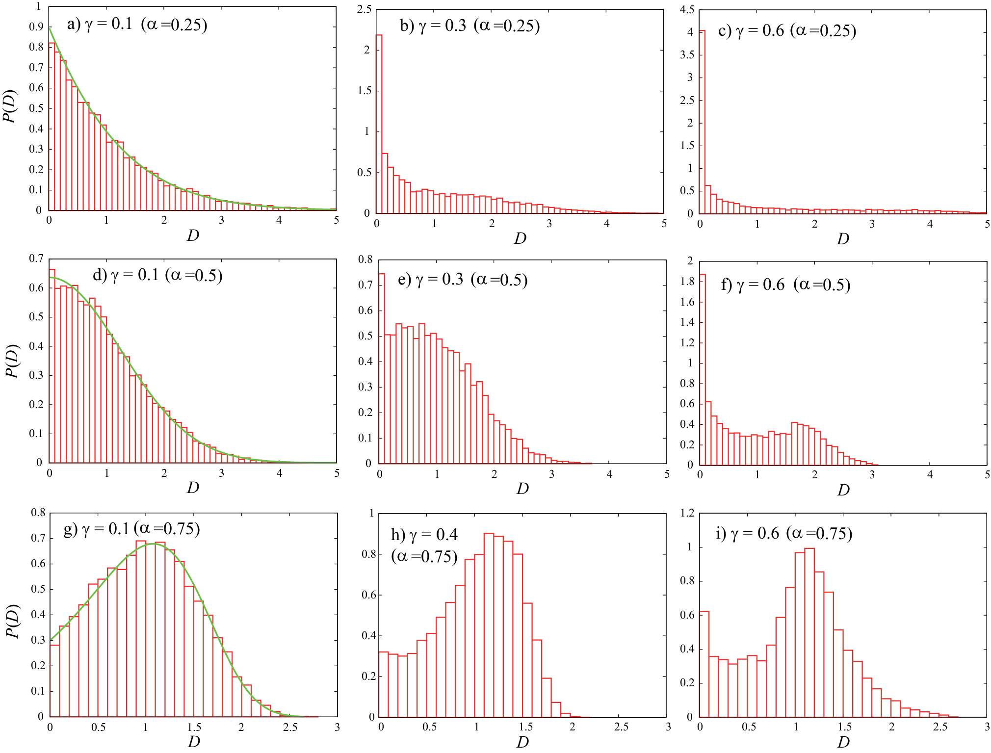
Moreover, for $2\gamma>\alpha$, the distribution of $D$ also converges to a time-independent non-trivial distribution as $t\to\infty$, indicating that the scaled diffusion coefficient converges to a random variable (i.e., distributional ergodicity). PDFs of the normalized diffusion coefficient $D$ for different parameters are shown in Fig. 6 by numerical simulations. PDFs depend crucially on the coupling parameter $\gamma$ for $2\gamma>\alpha$. We note that the PDF for $2\gamma<\alpha$ is exactly the same as the Mittag-Leffler distribution of order $\alpha$.

In conclusion, we have shown subdiffusion as well as superdiffusion in the SEDLF using Laplace analysis. By numerical simulations, we have presented the asymptotic behaviors of the PDF of the normalized positions in the SEDLF. This model (SEDLF) removes unphysical situations in Lévy flight such that the EAMSD always diverges. In the SEDLF, we have shown that TAMSDs increase linearly with time and the diffusion coefficients converge in distribution (distributional ergodicity). Distributions of the diffusion coefficients depends not only on the exponent $\alpha$ of the trapping-time distribution but also on the coupling exponent $\gamma$ for $2\gamma>\alpha$, and thus are different from those in separable CTRWs [11] as well as random walks with static disorder [14]. Especially, in superdiffusive regime $(\gamma>0.5)$, the mean diffusion coefficient enhances according to the increase of the measurement time.

References

• [1] A. Caspi, R. Granek, and M. Elbaum, Phys. Rev. Lett. 85, 5655 (2000).
• [2] I. Golding and E. C. Cox, Phys. Rev. Lett. 96, 098102 (2006).
• [3] A. Granéli, C. C. Yeykal, R. B. Robertson, and E. C. Greene, Proc. Natl. Acad. Sci. USA 103, 1221 (2006).
• [4] A. Weigel, B. Simon, M. Tamkun, and D. Krapf, Proc. Natl. Acad. Sci. USA 108, 6438 (2011).
• [5] J.-H. Jeon, V. Tejedor, S. Burov, E. Barkai, C. Selhuber-Unkel, K. Berg-Sørensen, L. Oddershede, and R. Metzler, Phys. Rev. Lett. 106, 048103 (2011).
• [6] S. C. Weber, A. J. Spakowitz, and J. A. Theriot, Proc. Natl. Acad. Sci. USA 109, 7338 (2012).
• [7] I. M. Zaid, M. A. Lomholt, and R. Metzler, Biophys. J. 97, 710 (2009).
• [8] R. Metzler and J. Klafter, Phys. Rep. 339, 1 (2000).
• [9] M. J. Saxton, Biophys. J. 92, 1178 (2007).
• [10] A. Lubelski, I. M. Sokolov, and J. Klafter, Phys. Rev. Lett. 100, 250602 (2008).
• [11] Y. He, S. Burov, R. Metzler, and E. Barkai, Phys. Rev. Lett. 101, 058101 (2008).
• [12] T. Miyaguchi and T. Akimoto, Phys. Rev. E 83, 062101 (2011a).
• [13] Y. Meroz, I. M. Sokolov, and J. Klafter, Phys. Rev. Lett. 110, 090601 (2013).
• [14] T. Miyaguchi and T. Akimoto, Phys. Rev. E 83, 031926 (2011b).
• [15] J. Aaronson, An Introduction to Infinite Ergodic Theory (American Mathematical Society, Providence, 1997).
• [16] T. Akimoto and T. Miyaguchi, Phys. Rev. E 82, 030102(R) (2010).
• [17] M. M. Meerschaert and E. Scalas, Physica A 370, 114 (2006).
• [18] A. Helmstetter and D. Sornette, Phys. Rev. E 66, 061104 (2002).
• [19] J. Klafter, A. Blumen, and M. F. Shlesinger, Phys. Rev. A 35, 3081 (1987).
• [20] M. Magdziarz, W. Szczotka, and P. Żebrowski, J. Stat. Phys. 147, 74 (2012).
• [21] J. Liu and J.-D. Bao, Physica A 392, 612 (2013).
• [22] M. Shlesinger, J. Klafter, and Y. Wong, J. Stat. Phys. 27, 499 (1982).
• [23] J. Bouchaud and A. Georges, Phys. Rep. 195, 127 (1990).
• [24] H. Scher and E. W. Montroll, Phys. Rev. B 12, 2455 (1975).
• [25] D. R. Cox, Renewal theory (Methuen, London, 1962).
• [26] Y. Kasahara, Publ. RIMS, Kyoto Univ. 12, 801 (1977).
• [27] T. Miyaguchi and T. Akimoto, Phys. Rev. E 87, 032130 (2013).
• [28] V. Tejedor and R. Metzler, J. Phys. A 43, 082002 (2010).
• [29] T. Akimoto, E. Yamamoto, K. Yasuoka, Y. Hirano, and M. Yasui, Phys. Rev. Lett. 107, 178103 (2011).
• [30] T. Uneyama, T. Akimoto, and T. Miyaguchi, J. Chem. Phys. 137, 114903 (2012).