Mean field games with nonlinear mobilities in pedestrian dynamicsThanks: MTW acknowledges financial support of the Austrian Science Foundation FWF via the Hertha Firnberg Project T456-N23. MDF is supported by the FP7-People Marie Curie CIG (Career Integration Grant) Diffusive Partial Differential Equations with Nonlocal Interaction in Biology and Social Sciences (DifNonLoc), by the ‘Ramon y Cajal’ sub-programme (MICINN-RYC) of the Spanish Ministry of Science and Innovation, Ref. RYC-2010-06412, and by the by the Ministerio de Ciencia e Innovación, grant MTM2011-27739-C04-02.
Abstract.
In this paper we present an optimal control approach modeling fast exit scenarios in pedestrian crowds.
In particular we consider the case of a large human crowd trying to exit a room as fast as possible.
The motion of every pedestrian is determined by minimizing a cost functional,
which depends on his/her position, velocity, exit time and the overall density of people.
This microscopic setup leads in the mean-field limit to a parabolic optimal control problem.
We discuss the modeling of the macroscopic optimal control approach and show how the optimal conditions relate
to Hughes model for pedestrian flow. Furthermore we provide results on the existence and uniqueness of minimizers
and illustrate the behavior of the model with various numerical results.
1. Introduction
Mathematical modeling of human crowd motion such as streetway pedestrian flows or the evacuation of large buildings is a topic of high practical relevance. The complex behavior of human crowds poses a significant challenge in the modeling and a majority of questions still remains open. Consequently it receives increasing attention, and in particular in the last years strong development in the mathematical literature becomes visible. A variety of different approaches has been proposed and partly analyzed, which can roughly be grouped as follows:
- (1)
- (2)
- (3)
- (4)
For evacuation scenarios an additional complication in the basic model arises, namely how the boundaries (i.e. doors, impermeable walls) and the goal of the pedestrians to leave the room as quickly as possible are modeled. A canonical approach is to use a potential force (or drift in random walk models) based on the distance function to the doors. This means that the potential solves some kind of Eikonal equation in the domain with zero Dirichlet boundary conditions on the part , which corresponds to the door. The appropriate statement of the Eikonal equation and its boundary conditions in a crowded situation is a delicate issue, which is mainly done in an ad-hoc fashion (even for detailed microscopic models) and has led to different directions. Some models simply use the distance function itself, i.e. the viscosity solution of
| (1.1) |
which corresponds to an overall optimization of the evacuation path independent of other pedestrians. This might be questionable in crowds due to limited visibility or global changes of the evacuation path to avoid jamming regions. Other models use variants of the Eikonal equation that incorporate the density of pedestrians. The celebrated Hughes model, cf. [28], uses an equation of the form
| (1.2) |
where is a function introducing saturation effects such as , where is a maximal density.
In this paper we introduce a rather unifying mean-field game approach to the modeling of evacuation scenarios, which links several of the above mentioned models and provides further understanding of several issues. This mean field framework provides interpretations of different forms of the Eikonal equation and covers the modeling of ‘realistic’ boundary conditions. We provide a detailed mathematical analysis and numerical simulations of our approach and discuss interesting special cases and limits, in particular its connection to Hughes’ model.
This paper is organized as follows: In Section 2 we present the modeling on the microscopic level and its mean-field limit. Furthermore we discuss its relation to Hughes’ model and the appropriate choice of boundary conditions. Section 3 is devoted to the analysis of the macroscopic optimal control approach. Finally we present a steepest descent approach to solve the parabolic optimal control problem in Section 4 and illustrate the behavior with several numerical examples.
2. Mathematical Modeling
In the following we discuss a model paradigm based on the idea of fast exit. At the single particle level, this yields a classical or stochastic optimal control problem, which we reformulate as PDE-constrained optimization model for the particle density. From the optimality conditions we then obtain a version of the Eikonal equation as the adjoint problem.
2.1. Fast Exit of Particles
Let us start with a deterministic particle (of unit mass) trying to leave the domain as fast as possible. Let denote the particle trajectory and
Then it makes sense to look for a weighted minimization of the exit time and the kinetic energy, i.e.
| (2.1) |
subject to , , where encodes the weighting of the fast exit.
Introducing the Dirac measure and a final time sufficiently large, we can rewrite the functional (2.1) as
| (2.2) |
subject to
| (2.3) |
and initial value . Note that for
and
which yields the equivalence between the particle formulation (2.1) and the continuum version (2.2) by the standard Lagrange-Euler transform of the velocity , cf. [27, 36].
Next we consider a stochastic particle, which moves according to the Langevin equation. Then we obtain
| (2.4a) | |||
| where a Wiener process and the diffusivity. It is natural to consider the stochastic optimal control problem | |||
| (2.4b) | |||
with the random variable determined by (2.4a) with initial value . Reformulating (2.4) for the distribution already reveals the structure of a mean-field game for the particle density. That is, writing we obtain the minimization functional
| (2.5a) | |||
| subject to | |||
| (2.5b) | |||
2.2. Optimality, Eikonal Equations, and Mean-Field Games
In the following we provide an explanatory derivation of the optimality conditions for the optimization problem
| (2.6) |
We shall derive the optimality condition at a formal level, without providing rigorous details on the functional setting and on the boundary conditions. We shall be more precise later on a more general model, see subsection 2.6.
We define the Lagrangian with dual variable as
| (2.7) |
For the optimal solution we have, in addition to (2.5b), the following equations, i.e.
| (2.8) |
and
| (2.9) |
with the additional terminal condition . Inserting we obtain the following system, which has the structure of a mean field game, i.e.
| (2.10a) | ||||
| (2.10b) | ||||
One observes the automatic emergence of a transient viscous Eikonal equation, which is to be solved backward in time with terminal condition. The connection to models using the distance function as a potential is quite apparent for a time interval with and . Noticing that the Hamilton-Jacobi equation is solved backwards in time and that the backward time is large for , we see that the solution is mainly determined by the large-time asymptotics (cf. [29]) solving
| (2.11) |
for some constant . Hence the potential becomes approximately a multiple of the distance function.
2.3. Mean Field Games and Crowding
We now turn our attention to a more general mean field game, respectively its optimal control formulation. We generalize the terms depending on the density for reasons to be explained in detail below to obtain
| (2.12a) | |||
| subject to | |||
| (2.12b) | |||
and a given initial value . The motivation for those terms is as follows:
- •
The function corresponds to nonlinear mobilities, which are frequently used in crowding models, e.g. derived from microscopic lattice exclusion processes (cf. [10] for a pedestrian case). Nonlinear mobilities have been derived in different settings and used also in different applications of crowded motion, e.g. ion channels [9, 11] or cell biology [35, 33, 19]. A typical form of is close to linear and increasing for small densities, while saturating and possibly decreasing to zero for larger densities.
- •
The function corresponds to transport costs created by large densities. In particular one may think of tending to infinity as tends towards a maximal density. As we shall see below however, changes in can also be related equivalently to changes in the mobility.
- •
A nonlinear function may model active avoidance of jams in the exit strategy, in particular by penalizing large density regions.
The optimality conditions of (2.12) can be (again formaly) derived via the Lagrange functional
| (2.13) |
For the optimal solution we have
| (2.14) |
and
| (2.15) |
with terminal condition . Inserting we obtain the optimality system
| (2.16a) | ||||
| (2.16b) | ||||
again a mean field game.
2.4. Momentum Formulation
In order to reduce ambiguities in the definition of a velocity and also to simplify the constraint PDE, we use a momentum or flux-based formulation in the following, cf. [2, 5]. The flux density (or momentum) is given by , hence the functional do be minimized in (2.12) becomes
| (2.17a) | |||
| with , subject to | |||
| (2.17b) | |||
We see the redundancy of and in the above formulation, effectively only determines different cases. We mention that in order to obtain a rigorous formulation, we replace in (2.17a) by
| (2.18) |
The Lagrange functional for this problem is given by
| (2.19) |
and the optimality conditions are
| (2.20a) | ||||
| (2.20b) | ||||
We recall that the rigorous formulation of the problem in terms of the boundary conditions will be performed in subsection 2.6.
2.5. Relation to the Hughes Model
For vanishing viscosity the optimality system (2.16) respectively (2.20) has a similar structure as Hughes model for pedestrian flow, see [28], which reads as
| (2.21a) | ||||
| (2.21b) | ||||
Hughes proposed that pedestrians seek the fastest way to the exit, but at the same time try to avoid congested areas. Let denote the maximum density, then
the function models how pedestrians change their direction and velocity due to the overall density. A common choice for example is .
To obtain the connection with the Hughes model we choose , , then (2.20)
reads as
| (2.22a) | ||||
| (2.22b) | ||||
For large we expect equilibration of backward in time. If we further consider , then for time of order one the limiting model (very formal) becomes
| (2.23a) | ||||
| (2.23b) | ||||
which is almost equivalent to Hughes model (2.21), if we set . Note that the difference is in the term , which is however severe. For we have
thus for small densities the behavior is similar, but the singular point is . A (so far partial) attempt to a rigorous mathematical theory for the original Hughes model (2.21) has been provided in [1]. Previous results [17, 15] considered smoothed version of that model. El-Khatib et al. first considered a variant with a cost in the eikonal equation not related to , cf. [21], and finally Gomes and Saude provided a priori estimates for (2.22) in [23].
2.6. Boundary Conditions
We finally turn to the modeling of the boundary conditions, which we have neglected in the computations above. To do so we consider (2.17) on a bounded domain , , corresponding to a room with one or several exits. We assume that the boundary is split into a Neumann part , modeling walls, and the exits , and . We now formulate natural boundary conditions on the density, which will lead to adjoint boundary conditions for .
On the Neumann boundary we clearly have no outflux, hence naturally
where denotes the unit outer normal vector. The exit part is more difficult. Here the outflux depends on how fast people can leave the room. If we denote the rate of passing the exit by , then we have the outflow proportional to . Hence, we arrive at the Robin boundary condition
| (2.24) |
Then boundary conditions for the adjoint variable can be calculated again from the optimality conditions. If we define the Lagrangian in this case we obtain:
| (2.25) |
In this form we see that the optimality condition with respect to , i.e. , yields the following boundary conditions for the adjoint variable in addition to the adjoint PDE:
| (2.26) |
One observes that our model provides meaningful and easily interpretative boundary conditions for the density as well as for the adjoint variable . A homogeneous Dirichlet boundary condition for on doors arises only in the asymptotic limit . In this case one also needs to specify a homogeneous Dirichlet boundary condition for for consistence. This is in contrast to previous models, which frequently used Dirichlet boundary conditions for , but arbitrary Dirichlet values for or an outflux boundary condition as above with finite .
In the case of Hughes model (2.21) commonly used boundary conditions are chosen as follows. The potential is assumed to satisfy homogeneous Dirichlet boundary conditions, i.e. , while the density either satisfies a Dirichlet boundary conditions of type or an outflux condition as in (2.24). There are two possibilities to compare the behavior of solutions of (2.21) and (2.22):
- •
Either by prescribing a density at the exit, i.e. and homogeneous Dirichlet boundary conditions for the adjoint, i.e. . This, however, is not realistic in practical applications.
- •
Or by choosing outflux boundary conditions for the density , as in (2.24) with a large proportionality constant , and the corresponding no-flux boundary conditions (2.26) in the for . The latter choice for the potential is not compatible with (2.21), but approximates the homogeneous Dirichlet boundary condition (typically chosen in Hughes model) for large.
Note that no flux boundary conditions for the density , i.e. in (2.24) would result in a homogeneous Neumann boundary conditions (2.26) for . Such boundary conditions are not compatible with the Eikonal equation (2.21b) in Hughes model and contradict the initial modeling assumptions.
3. Analysis of the Optimal Control Model
3.1. Existence of Minimizers
In this section we discuss the existence and uniqueness of minimizers for the optimization problem (2.12), respectively the reformulation (2.17). In order to avoid any ambiguity with the formulations we can simply set
which will remain as a standing assumption throughout the rest of this section. Let be a bounded domain in . We make the following basic assumption on and :
- (A1)
, bounded, and , for .
Existence of minimizers is guaranteed if
- (A2)
is convex.
As recalled in subsection 2.5, models with maximal density are of great importance in the applied setting, therefore we shall consider the special class of mobilities which yields a density uniformly bounded by a maximal density. Let us fix the maximal density to be . Let us denote by . Typically . In order to force the minimizers of the problem to satisfy , we extend to on . This defines the next assumption on , i.e.
- (A3)
if and otherwise.
Note that assumption (A3) is satisfied in particular by in the Hughes model in subsection 2.5. To show uniqueness we need another additional assumption for , namely
- (A4)
is concave.
We consider the optimization problem on the set , i.e. , where and are defined as follows
| (3.1) |
Hence the optimization problem (2.12) reads as
| (3.2) |
respectively in momentum formulation
| (3.3) |
In order to have the differential constraint well defined in the prescribed functional setting, and to incorporate the Robin boundary conditions in the statement of the problem, we shall provide a more rigorous definition of the minimization problem below.
For the existence proof in the case of non-concave , we introduce another formulation based on the rather nonphysical variable
which has been used already in the case of linear in [8]. Then the functional can be re-written as
| (3.4) |
and the optimization problem formally becomes
| (3.5) |
In order to make the relation among the problems (3.2), (3.3), and (3.5) rigorous, we need to extend the domain of the velocity to
| (3.6) |
Moreover, for given we define an extension mapping to via
| (3.7) |
With this notation, we easily get (we omit the details)
Lemma 3.1.
As a consequence of the above Lemma, we see that if one of the models has a minimizer with uniformly bounded away from zero, it is in and minimizes all three models. We are now ready to state the minimization problem (3.2) and its reformulation (3.5) rigorously, in a way to incorporate the Robin boundary conditions, and to take into account the proper functional setting.
Definition 3.2 (Minimisation problem, 1st formulation).
Let . A pair is a weak solution to the minimization problem (3.2) with initial condition , if and
| (3.8) |
for all , and if
A similar re-formulation of (3.3) in terms of the momentum variable replacing can be also deduced.
Definition 3.3 (Minimisation problem, 2nd formulation).
Similarly, on the variables setting we get:
Definition 3.4 (Minimisation problem, 3rd formulation).
Let . A pair is a weak solution to the minimization problem (3.5) with initial condition , if and
| (3.10) |
for all , and if
We now prove our main existence result in the formulation using , which allows also for non-concave , and relies on a positive viscosity . First, we provide an a-priori estimate:
Lemma 3.5.
Proof.
We use the test function and obtain
Since is bounded, the second to last term is non positive, and . This yields after integration in time
with a constant depending only on and . For the time derivative we deduce that
where the first term on the right-hand side includes the gradient terms in the domain as well as the boundary term via a trace theorem. Squaring and integrating in time finally yields the desired estimate for . ∎
The following technical Lemma is needed to ensure that assumption (A3) gives . We provide the details for the sake of completeness, although the result is quite standard.
Lemma 3.6.
Proof.
Assume first , and let be a regularization of the positive part as , such that , and . We can use the test function in Definition 3.4 to get
| (3.13) |
where
Now, it is clear that if . Moreover, for we have
since is uniformly bounded. Finally, in the case , we have
as . Combining all these assumptions, we get uniformly bounded and such that almost everywhere on . Since , we can integrate in time in (3.13) and send to get
which gives the assertion. The general case can be recovered by a standard approximation argument, we omit the details. ∎
Theorem 3.7 (Existence in the general case).
Proof.
We show the existence of a minimizer by the direct method. Let be a minimizing sequence. Then we can assume without loss of generality that there exists a constant , such that
Clearly, is bounded in and hence has a weakly convergent sub-sequence with limit , again denoted by . Now we use Lemma 3.5 to obtain boundedness of , from which we can extract another weakly convergent sub-sequence. From the Lemma of Aubin and Lions, cf. [34], we have a compact embedding of . Then the continuity and boundedness of implies that converges strongly in and the limit is bounded. Hence, the product converges weakly in and the limit is in , which allows to pass to the limit in the weak formulation of the constraint equation. Thus, is admissible, and the weak lower semicontinuity of the objective functional implies that it is indeed a minimizer. Note that the convexity of is crucial in this case, as it provides lower semi continuity of . Assume now that (A3) is satisfied. Then, due to Lemma 3.6 for all we have , which can be passed to the limit (possibly by extracting a further subsequence converging almost everywhere) to obtain the desired result. ∎
We now provide an alternative argument, which can be extended to the non-viscous case for zero-flux flux boundary conditions, i. e. for . The argument below provides less regularity for the minimizer compared to the previous result, but the proof is much shorter.
Theorem 3.8 (Existence for concave mobility).
Proof.
Let be a minimizing sequence. Since is bounded, is uniformly bounded in and we can extract a weakly convergent sub-sequence with limit . By the boundedness of the objective functional, we have almost everywhere, which gives for all and for all . From the latter we can extract a sub sequence, again denoted by such that in , respectively weakly in for . Since the constraint PDE is linear we can easily pass to the limit in a weak formulation and see that
holds in a weak sense. Moreover, the convexity of the objective functional guaranteed by (A2), (A3), and (A4) (recall that is extended to when ) implies weak semi-continuity an hence is a minimizer. The uniqueness follows from a standard strict convexity argument. ∎
Remark 3.9.
The result in Theorem 3.8 can be extended to the case in case the boundary conditions are posed with , i. e. no exits at the boundary. In this case, the boundary condition can be trivially passed to the limit above, whereas we are not able to close such argument in case . This case requires a more refined analysis based on the theory of nonlinear conservation laws with boundary conditions, cf. [4].
Remark 3.10.
We mention that under the above assumptions one might expect Gamma-convergence of the optimal control problems as . The lower semicontinuity arguments can be used to verify the lower bound inequality, however it is so far unclear how the upper bound inequality can be verified.
Note that the convexity constraint (A2) can be weakened, i.e. the function has to be weakly lower semicontinuous in suitable function spaces to guarantee existence of minimizers. Since we only consider convex functions , we did not state this more general result.
3.2. Adjoint Equations and Optimality System
In the following we investigate the existence of adjoints, i.e. the optimality condition with respect to the state variable :
Proposition 3.11.
Note that the right hand side of (3.14) is only in . Existence and uniqueness of solutions follows from the results of Boccardo and Gallouët, cf. [7]. However this result does not provide the necessary regularity for to define the Lagrange functional properly.
Finally we investigate the full optimality system, where we eliminate and obtain
| (3.15a) | ||||||
| (3.15b) | ||||||
| with boundary conditions | ||||||
| (3.15c) | ||||||
To show uniqueness of the forward backward system (3.15) we follow an approach proposed by Lasry and Lions for mean field games, cf. [31].
Theorem 3.12 (Uniqueness for the optimality system).
Proof.
Assume there exists two classical solutions and to the optimality system (2.16). We denote the difference between the solutions by and , which satisfy
| (3.16a) | ||||
| (3.16b) | ||||
Note that the differences and satisfy the following boundary conditions on :
| (3.17) |
Using (3.16) we calculate (integrating by parts):
Note that due to the boundary conditions (3.17), all boundary terms that result from the integration by parts in the previous calculation vanish. Due to the concavity of we deduce that
Since is in and convex, is monotone and we obtain
We integrate over the interval and obtain (since and ) that:
| (3.18) |
The function is positive, therefore (3.18) implies that
Then is a solution of and we conclude (by uniqueness) that . ∎
4. Numerical simulations
In this section we present a steepest descent approach for the solution of the parabolic optimal control problem (2.12). This method can be used for convex optimization problems and defines an iterative scheme to determine the optimal and .
The presented numerical simulations focus on the different behavior of the classical model of Hughes (2.21) and the corresponding general mean field modification (2.22). This comparison requires the simulation of (2.21), which is done using a finite volume scheme for the nonlinear conservation law and a fast sweeping method for the Eikonal equation, as presented by Di Francesco et al. in [17].
The steepest descent scheme for (2.12) can be written as:
Scheme 1.
Let , , where is the solution of the Eikonal equation in the classical Hughes model (2.21) with for all and , be the given initial data. Then the steepest descent scheme reads as:
- (1)
- (2)
Calculate the backward evolution of the adjoint variable using the previously calculated density in
with an implicit in time discretization and a MHDG method for the spatial discretization.
- (3)
Update the velocity via , where is a suitably chosen step size.
- (4)
Go to (1) until convergence of the function (2.12a).
Egger and Schöberl presented a MHDG method for linear convection dominated problems, which can be adapted for the nonlinear problems considered. We use the following basis functions for the discretization, i.e.
where denotes piecewise constant basis function on the interval and lowest order Raviart-Thomas basis functions. The Newton iteration in (4.1) is terminated, if .
Throughout this section we consider the domain with exits located at . The interval is divided into a set of equidistant intervals of length . Furthermore the maximum density is set to .
4.1. Comparison of the classical and the mean field type Hughes model
We have seen in Section 2.5 that the proposed mean field model has a similar structure as the classical model by Hughes. Hence we want illustrate the behavior of both models with various experiments. In the first example we focus on the influence of the boundary conditions as discussed in Section 2.6. In the second example we illustrate the basic difference of the mean field game approach and the classical model of Hughes.
4.1.1. Behavior for different values of
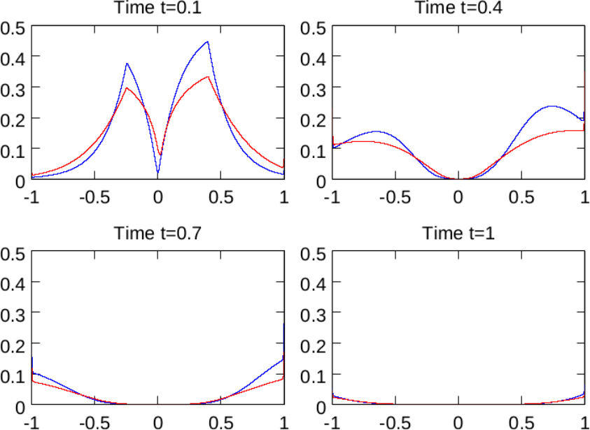
We consider the time interval . In the classical Hughes model (2.21) the boundary conditions are set to
with . For the corresponding mean field model (2.22) the functions and satisfy (2.24) and (2.26) at . In both cases we use the same diffusion coefficient, i.e . The spatial discretization is set to in (2.21) and in (2.22), the time steps to and respectively. The different magnitudes of the time stepping can be explained by the explicit in time discretization of (2.21) and the implicit time discretization of (2.22). Figures 1 and 2 show the evolution in time of the solutions of (2.21) and (2.22) for different values of . Although the models have a very similar structure, their behavior is different. In the mean field model small congestions at the boundary are visible for . Furthermore we do not observe the immediate vacuum formation at as in Hughes model (2.21). People rather tend to “wait for a little while” at the center and then start to move at a higher speed. The expected equilibration of in (2.22) is clearly visible in Figure 2 for all values of .


4.1.2. Fast exit of several groups
In this example we consider three groups, which want to leave the domain as fast as possible. The particular initial datum is given by
A similar example was already considered in [17], where the simulations showed that the
a small part of the group located around initially splits to move to the exit at , but later
on turns around to take the closer exit at . This behavior can be explained by the fact that
the pedestrians in Hughes model (2.21), adapt their velocity in every time step (depending
on the overall density at that time). Due to the initially high density of people located in front of exit
, parts of the group start to move towards , but turn around when the density is decreasing
as more and more people exit.
We do not expect to observe this behavior for the modified Hughes model (2.22). One of
the underlying features of the proposed optimal control approach, is the fact that each pedestrian knows the distribution
of all other people at all times. Therefore he/she is anticipating the behavior of the group in the
future and will in this case rather wait than move to the more distant exit. This expected behavior can be observed
in Figure 3.


Here the mean field model (2.22) was solved using the steepest descent approach detailed before. The parameters were set to:
Note that the optimal control formulation of (2.22) is not a convex problem (the function is only concave for ), but the steepest descent approach converged without any problems. For Hughes model we chose the following parameters:
4.2. Linear vs. nonlinear
In the final example we illustrate the behavior for different functions . In particular we set
The later choice of actively penalizes regions of high density and urges the group to get out more efficiently. In this example the group is initially located at
The parameters are given by and . Figure 4 shows the evolution of the density for the different choices of in time. As expected we observe that the group exits much faster and spreads out more evenly for than in the linear case.
Conclusion
In this paper we presented a novel mean field game approach for evacuation and fast exit situations in crowd motion. We motivated the model on the microscopic level and discussed its generalization in the mean field limit. The optimality system of the resulting parabolic optimal control problem, is a mean field game and establishes interesting links to well known models, like Hughes model for pedestrian flow. Furthermore the proposed model gives new insights into the mathematical modeling of boundary conditions for pedestrian crowds. We present first existence and uniqueness results for the proposed optimal control approach and illustrate the behavior of solutions with various numerical simulations.
The general formulation of the proposed model poses interesting challenges for future research. In general the derivation of mean-field limit with nonlinear mobilities is of significant importance and raised a lot of interest in the scientific community, cf. e.g. [13]. In addition challenging questions and problems arise in the mathematical analysis of the optimal control approach for convex as well as non-convex problems. Another important direction of research will focus on more realistic modeling assumptions. We have seen in the second example of Section 4 that people anticipate the density of all others in time, which is questionable in many situations. Therefore it would be interesting to study the behavior of (2.12) with a temporal discount factor, as proposed in [30]. Finally the development of a numerical solver for 2D problems and its generalization to non-convex problems would allow for more realistic simulations.
References
- [1] D. Amadori and M. Di Francesco, The one-dimensional Hughes model for pedestrian flow: Riemann-type solutions, Acta Math. Sci. Ser. B Engl. Ed., 32 (2012), pp. 259–280.
- [2] L. Ambrosio, S. Lisini, and G. Savare, Stability of flows associated to gradient vector fields and convergence of iterated transport maps, Manuscripta Math., 121 (2006), pp. 1–50.
- [3] C. Appert-Rolland, P. Degond, and S. Motsch, Two-way multi-lane traffic model for pedestrians in corridors, Netw. Heterog. Media, 6 (2011), pp. 351–381.
- [4] C. Bardos, A. Y. le Roux, and J.-C. Nédélec, First order quasilinear equations with boundary conditions, Comm. Partial Differential Equations, 4 (1979), pp. 1017–1034.
- [5] J.-D. Benamou and Y. Brenier, A computational fluid mechanics solution to the Monge-Kantorovich mass transfer problem, Numer. Math., 84 (2000), pp. 375–393.
- [6] V. J. Blue and J. L. Adler, Cellular automata microsimulation for modeling bi-directional pedestrian walkways, Transportation Research Part B: Methodological, 35 (2001), pp. 293 – 312.
- [7] L. Boccardo and T. Gallouët, Nonlinear elliptic and parabolic equations involving measure data, J. Funct. Anal., 87 (1989), pp. 149–169.
- [8] C. Brune, 4D Imaging in Tomography and Optimal Nanoscopy, PhD thesis, University of Münster, 2010.
- [9] M. Burger, M. Di Francesco, J.-F. Pietschmann, and B. Schlake, Nonlinear cross-diffusion with size exclusion, SIAM J. Math. Anal., 42 (2010), pp. 2842–2871.
- [10] M. Burger, P. A. Markowich, and J.-F. Pietschmann, Continuous limit of a crowd motion and herding model: analysis and numerical simulations, Kinet. Relat. Models, 4 (2011), pp. 1025–1047.
- [11] M. Burger, B. Schlake, and M.-T. Wolfram, Nonlinear Poisson-Nernst-Planck equations for ion flux through confined geometries., Nonlinearity, 25 (2012), pp. 961–990.
- [12] C. Burstedde, K. Klauck, A. Schadschneider, and J. Zittartz, Simulation of pedestrian dynamics using a two-dimensional cellular automaton, Physica A: Statistical Mechanics and its Applications, 295 (2001), pp. 507 – 525.
- [13] R. Carmona and F. Delarue, Probabilistic analysis of mean-field games, 2012.
- [14] M. Chraibi, A. Wagoum, A. Schadschneider, and A. Seyfried, Force-based models of pedestrian dynamics, NHM, 6 (2011), pp. 425–442.
- [15] R. M. Colombo, M. Garavello, and M. Lécureux-Mercier, A class of nonlocal models for pedestrian traffic, Math. Models Methods Appl. Sci., 22 (2012), pp. 1150023, 34.
- [16] R. M. Colombo, P. Goatin, and M. D. Rosini, A macroscopic model for pedestrian flows in panic situations, in Current advances in nonlinear analysis and related topics, vol. 32 of GAKUTO Internat. Ser. Math. Sci. Appl., Gakkōtosho, Tokyo, 2010, pp. 255–272.
- [17] M. Di Francesco, P. A. Markowich, J.-F. Pietschmann, and M.-T. Wolfram, On the Hughes’ model for pedestrian flow: the one-dimensional case, J. Differential Equations, 250 (2011), pp. 1334–1362.
- [18] C. Dogbé, Modeling crowd dynamics by the mean-field limit approach, Math. Comput. Modelling, 52 (2010), pp. 1506–1520.
- [19] L. Dyson, P. Maini, and R. Baker, Macroscopic limits of individual-based models for motile cell populations with volume exclusion., Phys. Rev. E Stat. Nonlin. Soft Matter Phys., 86 (2012), p. 031903.
- [20] H. Egger and J. Schöberl, A hybrid mixed discontinuous Galerkin finite-element method for convection diffusion problems, IMA Journal of Numerical Analysis, 30 (2010), pp. 1206–1234.
- [21] N. El-Khatib, P. Goatin, and M. D. Rosini, On entropy weak solutions of hughes’ model for pedestrian motion, Z. Angew. Math. Phys., 64 (2012), pp. 223–251.
- [22] P. Goatin and M. Mimault, The wave-front tracking algorithm for Hughes’ model of pedestrian motion, SIAM J. Sci. Comput., (2012). accepted for publication.
- [23] D. Gomes and J. Saúde, Mean field games - a brief survey, tech. rep., submitted, 2013.
- [24] O. Guéant, J.-M. Lasry, and P.-L. Lions, Mean field games and applications, in Paris-Princeton Lectures on Mathematical Finance 2010, vol. 2003 of Lecture Notes in Math., Springer, Berlin, 2011, pp. 205–266.
- [25] D. Helbing, I. Farkas, and T. Vicsek, Simulating dynamical features of escape panic, Nature, 407 (2000), pp. 487–490.
- [26] D. Helbing and P. Molnar, Social force model for pedestrian dynamics, Physical Review E, 51 (1998), pp. 4282–4286.
- [27] S. P. Hoogendoorn and P. H. L. Bovy, Pedestrian route-choice and activity scheduling theory and models, Transportation Research Part B: Methodological, 38 (2004), pp. 169–190.
- [28] R. L. Hughes, A continuum theory for the flow of pedestrians, Transportation Research Part B: Methodological, 36 (2002), pp. 507 – 535.
- [29] H. Ishii, Asymptotic solutions for large time of hamilton–jacobi equations in euclidean n space, Annales de l’Institut Henri Poincare (C) Non Linear Analysis, 25 (2008), pp. 231 – 266.
- [30] A. Lachapelle and M.-T. Wolfram, On a mean field game approach modeling congestion and aversion in pedestrian crowds, Transportation Research Part B: Methodological, 45 (2011), pp. 1572 – 1589.
- [31] J.-M. Lasry and P.-L. Lions, Mean field games, Jpn. J. Math., 2 (2007), pp. 229–260.
- [32] M. Moussaïd, E. G. Guillot, M. Moreau, J. Fehrenbach, O. Chabiron, S. Lemercier, J. Pettré, C. Appert-Rolland, P. Degond, and G. Theraulaz, Traffic instabilities in self-organized pedestrian crowds, PLoS Comput. Biol., 8 (2012), p. e1002442.
- [33] K. J. Painter and T. Hillen, Volume-filling and quorum-sensing in models for chemosensitive movement., Can. Appl. Math. Q., 10 (2002), pp. 501–543.
- [34] R. E. Showalter, Monotone operators in Banach space and nonlinear partial differential equations, vol. 49 of Mathematical Surveys and Monographs, American Mathematical Society, Providence, RI, 1997.
- [35] M. Simpson, B. Hughes, and K. Landman, Diffusing populations: Ghosts or folks, Australasian Journal of Engineering Education, 15 (2009), pp. 59–68.
- [36] J. van den Berg, S. Patil, J. Sewall, D. Manocha, and M. Lin, Interactive navigation of multiple agents in crowded environments, in Proceedings of the 2008 symposium on Interactive 3D graphics and games, ACM, 2008, pp. 139–147.