CERN-PH-TH/2013-061

FERMILAB-PUB-13-063-T

Introduction. The determination of the spin $J$ and parity $P$ of the putative Higgs boson [1] is of paramount importance. The observed decay to $\gamma\gamma$ [2] already excludes the case of $J=1$ by the Landau-Yang theorem [3]. Spin discrimination and coupling measurements are achieved by studying kinematic correlations of the final state objects, generally leptons. An optimal way of incorporating all available information is through the Matrix Element Method (MEM) [4, 5, 7, 6]. Initial results from ATLAS [8] and CMS  [9, 10] strongly disfavor $J^{P}=0^{-}$, as well as $J^{P}=2^{+}$ with graviton-like couplings. These results represent an important first foray into the general parameter space of generic boson couplings.

In this paper we provide a theoretical framework for spin and coupling measurements in full generality, without theoretical prejudice towards specific benchmarks. In contrast to recent global fits of Higgs couplings [11, 12], our approach is geared towards a more model independent measurement in a single channel, including all relevant operators and utilizing all available kinematic information. For concreteness and simplicity, we consider the example of a spin-zero “$X$” resonance, decaying to four leptons through two intermediate $Z$-bosons [13, 14, 15, 16], though our approach can be readily extended to other spins and final states. The complete measurement of the $X$ couplings in full generality will provide insights into the nature of electroweak symmetry breaking and may offer the first glimpses of physics beyond the Standard Model (SM).

Effective Theory. In what follows, we will consider a spin-zero state $X$. In general, $X$ has no definite CP properties, and can be thought of as a linear combination of some $CP$-even state $H$ and some $CP$-odd state $A$ [12]:

In the special case of $\alpha=0$, $X$ is a pure $J^{P}=0^{+}$ scalar, as predicted in the Standard Model, while for $\alpha=\pm\pi/2$, $X$ is a pure pseudoscalar with $J^{P}=0^{-}$.

The $X$ couplings to two gauge bosons (e.g. $ZZ$) can be classified according to their symmetries in the $CP$-eigenstate basis $(H,A)$. Three types of terms are possible:

where $F^{\mu\nu}$ is the $Z$-boson field strength tensor, $M_{Z}=91.1876$ GeV is the $Z$-boson mass, $v=246$ GeV is the electroweak scale, and $\hat{f}^{(H)}$ and $\hat{f}^{(A)}$ are (in general momentum-dependent) form-factors, which from the effective theory point of view should be thought of as infinite series expansions in terms of some new physics scale $\Lambda$. Let us discuss each one in turn.

The form-factor $\hat{f}^{(H)}_{\mu\nu}$ describes interactions of the CP even component $H$ that necessarily violate $SU(2)$ gauge invariance. Expanding in powers of $\Lambda^{-1}$, one obtains

where $g_{i}$ are dimensionless coupling constants, and the derivative operator $\vec{\reflectbox{$\partial$}}$ ($\vec{\partial}$) acts on the $Z$ field to its left (right). Eq. (3) does not include terms containing $\partial^{\mu}Z_{\mu}$, which vanish in the Lorenz gauge.

The second class of $CP$-even couplings, described by the form-factor

may respect $SU(2)$ gauge invariance, if $H$ is a SM singlet. Note that terms of this sort could be generated by a $\left(\vec{\partial}_{\mu}\reflectbox{$\vec{\reflectbox{$\partial$}}$}_{\nu}-g_{\mu\nu}\vec{\partial}^{\rho}\reflectbox{$\vec{\reflectbox{$\partial$}}$}_{\rho}\right)$ term in Eq. (3), which explains the absense of such a term there. Finally, the couplings of the $CP$-odd component $A$ are given by

and may be $SU(2)$ gauge invariant as well, if $A$ is a SM singlet. However, here we do not make any assumptions about the $SU(2)$ quantum numbers of $H$ and $A$; the terms (4) and (5) will also violate $SU(2)$ gauge invariance if $H$ or $A$ (respectively) transform under $SU(2)$.

We note that the $g_{5}$ and $g_{6}$ terms in (3) are typically omitted in the literature. The contributions to the $X\to ZZ$ amplitude resulting from the $\reflectbox{$\vec{\reflectbox{$\Box$}}$}+\vec{\Box}$ and $\vec{\partial}^{\rho}\reflectbox{$\vec{\reflectbox{$\partial$}}$}_{\rho}$ terms are proportional to $M_{Z_{1}}^{2}+M_{Z_{2}}^{2}$ and $M_{X}^{2}-M_{Z_{1}}^{2}-M_{Z_{2}}^{2}$, respectively, where $M_{X}$ is the mass of the resonance and $M_{Z_{1}}$ and $M_{Z_{2}}$ are the invariant masses of the two $Z$-bosons (in the usual convention where $M_{Z_{1}}>M_{Z_{2}}$). Thus, if both $Z$-bosons were on-shell, the contribution from such terms would be essentially constant, and therefore could be absorbed into a redefinition of $g_{1}$. However, in the case of interest where $M_{X}\approx 125$ GeV, one or both of the $Z$’s are off-shell and $M_{Z_{1}}$ and $M_{Z_{2}}$ vary from event to event. Thus, strictly speaking, the $g_{5}$ and $g_{6}$ terms cannot be absorbed into $g_{1}$, though their effects (relative to $g_{1}$) are expected to be rather small, due to the additional $\Lambda^{2}$ suppression.

It appears that a general analysis of the couplings of the Higgs boson candidate would have to include at the very minimum the terms identified in eqs. (3-5), and perhaps even the higher dimensional operators $\sim\Lambda^{-4},\Lambda^{-5},\ldots$ which were not explicitly listed. Such an analysis may indeed be desirable at some point in the future, when significantly more data will have been accumulated by the LHC experiments. However, there are strong theoretical and experimental motivations for making certain simplifying assumptions for analyses in the immediate future.

First, all experimental evidence so far suggests that the new physics scale $\Lambda$ is high compared to $v$. Second, consistency of the effective theory description requires that $\Lambda$ be sufficiently removed from the relevant experimental energy scale. Finally, the higher dimensional nature of the $1/\Lambda$ couplings suggests a radiative origin and hence suppressions by loop factors. It is therefore reasonable to expect that the higher order terms $g_{3}$, $g_{5}$, $g_{6}$, etc. in the expansions (3-5) are negligible relative to the corresponding leading order couplings $g_{1}$, $g_{2}$ and $g_{4}$.

At the same time, the relative size of the leading terms $g_{1}$, $g_{2}$ and $g_{4}$ is a priori unknown. For example, the $g_{2}$ and $g_{4}$ terms are equally suppressed by $\Lambda$, and may both preserve gauge invariance, thus it is difficult to argue that one should be preferred over the other. Similarly, we do not know the extent to which $H$ is involved in breaking $SU(2)$ gauge invariance, and hence we cannot simply assume that the $SU(2)$ breaking term $g_{1}$ dominates over $g_{2}$, in spite of the additional $\Lambda$ suppression in the latter [15]. This is why we keep all three terms and consider the effective Lagrangian for the mass eigenstate $X$ to be

where $\tilde{F}_{\mu\nu}=\frac{1}{2}\varepsilon_{\mu\nu\rho\sigma}F^{\rho\sigma}$ and

are the effective couplings which need to be measured by experiment. We note that this procedure means neglecting (for the reasons stated above) the $g_{3}$ operator from Refs. [5, 6] and the $g_{5}$ and $g_{6}$ terms listed in (3).

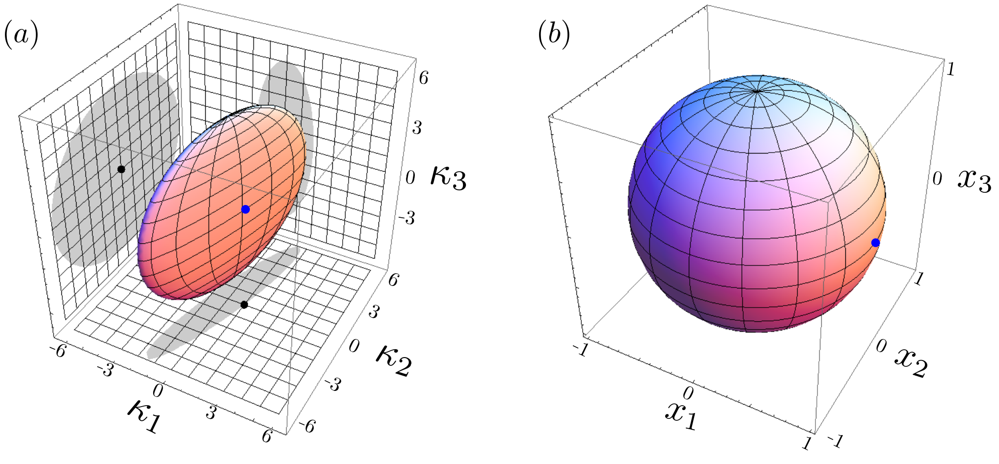
Counting degrees of freedom. From an effective theory point of view, the coefficients $\kappa_{i}$ in the Lagrangian (6) are real numbers. Thus the problem of measuring the Higgs couplings is reduced to determining the three dimensionless degrees of freedom $\kappa_{i}$. However, one can go one step further and use the measured signal rate ($X$ production cross-section times branching fraction for $X\to ZZ$) to eliminate one more degree of freedom, namely the overall $\kappa$ scale. In order to do this, we will assume that the $X$ can be treated as a narrow resonance. We then note that the partial width for $X\to ZZ$ is a quadratic function of the $\kappa$’s:

where we have factored out the partial width $\Gamma_{SM}$ predicted in the SM in order to define dimensionless coefficients $\gamma_{ij}$ listed in Table 1. The measured total rate then provides the overall normalization and constrains the $\kappa_{i}$ couplings to lie on the closed hyper-surface shown in Fig. 1(a). The idea now is to change variables and parameterize the couplings $\kappa_{i}$ in terms of the two coordinates on this hyper-surface. This re-parametrization is useful and meaningful, since the (normalized) angular and invariant mass distributions used to measure the Higgs spin and CP properties are insensitive to the overall scale of the couplings $\kappa_{i}$.

Operationally, we propose to do this by changing variables as

where $O_{21}=O_{31}=O_{32}=0$ and

In terms of the new variables $x_{i}$, the constraint implied by (8) is the surface of a sphere, as seen in Fig. 1(b).

Note that in the case of real couplings, $\gamma_{13}$ and $\gamma_{23}$ vanish identically (and hence are not listed in (8)). This can be understood in terms of parity; interference terms between amplitudes describing the decay of a parity-even scalar and a parity-odd scalar are odd under parity, hence vanish under integration provided the cuts respect parity (as is nearly always the case). The situation in the presence of cuts is less clear if the couplings of the three operators in (6) are complex valued; however, any $\gamma_{13}$ or $\gamma_{23}$ term generated in this case is expected to be very small.

Geolocating the Higgs. A sphere may be parameterized using latitude $\phi$ and longitude $\lambda$. Making an obvious analogy, we can think of the tree-level SM Higgs couplings $(\kappa_{1},\kappa_{2},\kappa_{3})=(1,0,0)$ as being represented by the point $(\phi,\lambda)=(0,0)$ in the Gulf of Guinea (see Fig. 2). The case of a pure pseudoscalar with $(\kappa_{1},\kappa_{2},\kappa_{3})=(0,0,1)$ corresponds to the North pole with $(\phi,\lambda)=(90,0)$. Those are the two main benchmark scenarios considered so far by the LHC experiments. The Higgs sphere from Fig. 1(b) now opens up the full range of possibilities. For example, one may consider a certain amount of mixing as in (1) between the SM Higgs and a pseudoscalar, placing us on the Greenwich meridian. Alternatively, one may allow non-trivial values for the two $CP$-even couplings $\kappa_{1}$ and $\kappa_{2}$, thus spanning the equator. Finally, one could also envision the most general case with non-trivial values for all three couplings, e.g. $(\kappa_{1},\kappa_{2},\kappa_{3})=(-0.945804,-3.88525,2.44522)$, corresponding to $(\phi,\lambda)=(29.64945,-82.3486)$, which happens to be a location in the south end zone of the Swamp.

We note that CMS has recently undertaken [10] an exploration of the sphere along the Greenwich meridian ($\lambda=0$) by measuring the parameter $f_{a3}\equiv|A_{3}|^{2}/(|A_{3}|^{2}+|A_{1}|^{2})$, parametrizing the relative contributions $|A_{1}|^{2}$ and $|A_{3}|^{2}$ to the total cross-section of the two benchmark models $(\kappa_{1},\kappa_{2},\kappa_{3})=(1,0,0)$ and $(\kappa_{1},\kappa_{2},\kappa_{3})=(0,0,1)$, respectively.

Selection cut bias. By definition, the measurement of the Higgs signal rate (and, by association, of the partial width (8)) is done using only events which pass selection cuts. Therefore, it needs to be corrected for the efficiency. Unfortunately, as demonstrated in the bottom right panel in Fig. 2, the signal efficiency is noticeably model dependent, i.e. it is quite sensitive to the actual values of the individual $\kappa_{i}$ parameters, and may vary from as low as $35\%$ to as high as $54\%$. One source of this variation is the cut on $M_{Z_{2}}$ (see e.g. [13]). The effect is quantified in Fig. 3, which shows unit-normalized $M_{Z_{2}}$ distributions for several choices of $\kappa_{i}$, including an example with a high efficiency ($(\kappa_{1},\kappa_{2},\kappa_{3})=(0,0,1)$, black circles) and a suitably chosen example with a low efficiency ($(\kappa_{1},\kappa_{2},\kappa_{3})=(1.8,5,0.08)$, red crosses). The $M_{Z_{2}}$ distribution in the latter case is softer, and many events fall below the minimum accepted $M_{Z_{2}}$ value of 12 GeV. We conclude that it would be virtually impossible to correct for the efficiency without knowledge of the couplings $\kappa_{i}$, which we are trying to measure in the first place, thus falling into a vicious circle.

Here we advocate an alternative approach. It is sufficient to realize that the coefficients $\gamma_{ij}$, while also affected by the efficiency, do not depend on $\kappa_{i}$. Therefore, in defining the Higgs sphere (9) one could simply use the corresponding values of $\gamma_{ij}$ after cuts, which need to be calculated once and for all. As shown in Table 1, the changes are subtle, yet noticeable. Note that even without any cuts, the same flavor (SF) and different flavor (DF) coefficients are different, due to the interference effects present in the SF case (see, e.g. [6]).

Interpretation. We emphasize that by studying the angular and invariant mass distributions of the final state leptons in the $X\to ZZ\to 4\ell$ channel it is experimentally possible to determine the exact geolocation of the Higgs boson candidate, without any simplifying theoretical assumptions. A proof of principle is shown in Fig. 4. We consider 4 benchmark scenarios for $(\kappa_{1},\kappa_{2},\kappa_{3})$: ($\triangle$) $(1,0,0)$, ($\circ$) $(0,1,0)$, ($\star$) $(0,0,1)$, and ($+$) $(1,1,1)$. We show results from 1000 pseudoexperiments with 300 signal events each (after cuts). Fig. 4 shows that in each case, the maximum likelihood fit indeed selects the correct geolocation (marked with an open symbol) of the Higgs candidate.

(In)determination of the mixing angle $\alpha$. We note that geolocating the Higgs candidate by itself is not sufficient to determine the value of the mixing angle $\alpha$, and we will still not know the relative composition of $X$ in terms of $H$ and $A$. As seen in eq. (7), the measurement of all three effective couplings $\kappa_{1}$, $\kappa_{2}$ and $\kappa_{3}$ only places 3 constraints on the 4 input parameters $\alpha$, $g_{1}$, $g_{2}/\Lambda$ and $g_{4}/\Lambda$, so one degree of freedom (which can be chosen to be the mixing angle $\alpha$) will always be left undetermined.

Music of the Spheres. Until now, we have been treating the coefficients $\kappa_{i}$ of the operators in the effective Lagrangian (6) to be real. We term this “Scenario 0”. Of course, this must be the case at tree level, and even beyond, as long as those operators are generated by loop diagrams involving heavy particles, such as the top, which may be consistently integrated out of the full theory to form an effective theory. However, in accordance with the optical theorem, loops with light particles (such as $b$-quarks, which cannot be integrated out of the theory) will contribute imaginary parts to those couplings. In this case, each of the $\kappa_{i}$ is complex and there are five physical degrees of freedom (an overall phase in the $\kappa_{i}$ may be removed). Nevertheless, the width constraint $\Gamma(X\to ZZ)=\Gamma_{SM}\sum_{i,j}\gamma_{ij}\kappa_{i}^{\ast}\kappa_{j}$ can still be enforced. As before, the diagonalization and rescaling (9) renders this a sphere in $\mathbb{C}^{3}$ (rather than an ellipsoid, as is the case in general).

Even in this general complexified case, there are three interesting and simple scenarios where the number of degrees of freedom is reduced to three. Namely, if one of $\kappa_{i}$ is too small to have observable effects, then the remaining two $\kappa_{i}$, taken to be arbitrary complex numbers, also comprise two observable degrees of freedom (as an overall phase may be removed). There are, of course three such scenarios, “Scenario 1” where $\kappa_{1}$ is negligible, “Scenario 2” where $\kappa_{2}$ is negligible, and “Scenario 3” where $\kappa_{3}$ is negligible.

Other final state channels. While we have so far only focused on the $ZZ\to 4\ell$ final state, the preceding discussion can be readily applied to the other di-boson final states, $W^{+}W^{-}$, $Z\gamma$, and $\gamma\gamma$. The interactions relevant for those channels involve corresponding new couplings $\kappa_{i}^{\tiny WW}$, $\kappa_{i}^{\tiny Z\gamma}$, and $\kappa_{i}^{\tiny\gamma\gamma}$. Assuming $SU(2)$ gauge symmetry, these new couplings are related, e.g.

with obvious definitions of $\kappa$’s. As before, the measured rate in each of those channels defines a sphere similar to eq. (8), where the corresponding values for the coefficients $\gamma_{ij}$ are given in Table 1. It is interesting to note that these spheres are not overlapping (even for the DF and SF case in the same $X\to ZZ$ channel), and in principle couplings can be measured from intersecting spheres, although we expect that this method is of only academic interest, since the corresponding precision would be very poor.

Summary. We have proposed several related parameterizations of the couplings of the $125$ GeV boson discovered at the LHC. These parameterizations allow the LHC experiments to go beyond comparing benchmark points, etc. in a relatively simple, yet very general, theoretically motivated fashion. The low dimensionality of the parameter space is helpful experimentally as well as in the visualization and interpretation of results. We look forward to the implementation of this method by the LHC collaborations and to the continued exploration of the couplings of the putative Higgs boson.

Acknowledgements. We thank A. Gritsan, A. Korytov, I. Low, and G. Mitselmakher for useful discussions. JG, JL, KM and SM thank their CMS colleagues. JL acknowledges the hospitality of the SLAC Theoretical Physics Group. MP is supported by the CERN-Korea fellowship through the National Research Foundation of Korea. Work supported in part by U.S. Department of Energy Grants DE-FG02-97ER41029. Fermilab is operated by the Fermi Research Alliance under contract DE-AC02-07CH11359 with the U.S. Department of Energy.

References

- [1] G. Aad et al. [ATLAS Collaboration], Phys. Lett. B 716, 1 (2012) [arXiv:1207.7214 [hep-ex]]; S. Chatrchyan et al. [CMS Collaboration], Phys. Lett. B 716, 30 (2012) [arXiv:1207.7235 [hep-ex]].
- [2]
ATLAS Collaboration,
ATLAS-CONF-2013-012,
http://cdsweb.cern.ch/record/1523698; ATLAS Collaboration, ATLAS-CONF-2013-029,http://cdsweb.cern.ch/record/1527124; CMS Collaboration, CMS-PAS-HIG-13-001,http://cdsweb.cern.ch/record/1530524. - [3] L. D. Landau, Dokl. Akad. Nauk Ser. Fiz. 60, 207 (1948); C.-N. Yang, Phys. Rev. 77, 242 (1950).
- [4] K. Kondo, J. Phys. Soc. Jap. 57, 4126 (1988) and 60, 836 (1991); R. H. Dalitz and G. R. Goldstein, Phys. Rev. D 45, 1531 (1992); B. Abbott et al. [DØ Collaboration], Phys. Rev. D 60, 052001 (1999); V. M. Abazov et al. [DØ Collaboration], Nature 429, 638 (2004).
- [5] Y. Gao, A. V. Gritsan, Z. Guo, K. Melnikov, M. Schulze and N. V. Tran, Phys. Rev. D 81, 075022 (2010) [arXiv:1001.3396 [hep-ph]]; S. Bolognesi, Y. Gao, A. V. Gritsan, K. Melnikov, M. Schulze, N. V. Tran and A. Whitbeck, Phys. Rev. D 86, 095031 (2012) [arXiv:1208.4018 [hep-ph]].
- [6] P. Avery, D. Bourilkov, M. Chen, T. Cheng, A. Drozdetskiy, J. S. Gainer, A. Korytov and K. T. Matchev et al., Phys. Rev. D 87, 055006 (2013) arXiv:1210.0896 [hep-ph].
- [7] A. De Rujula, J. Lykken, M. Pierini, C. Rogan and M. Spiropulu, Phys. Rev. D 82, 013003 (2010) [arXiv:1001.5300 [hep-ph]]; J. S. Gainer, K. Kumar, I. Low and R. Vega-Morales, JHEP 1111, 027 (2011) [arXiv:1108.2274 [hep-ph]]; J. M. Campbell, W. T. Giele and C. Williams, arXiv:1205.3434 [hep-ph]; J. M. Campbell, W. T. Giele and C. Williams, JHEP 1211, 043 (2012) [arXiv:1204.4424 [hep-ph]]; D. Stolarski and R. Vega-Morales, Phys. Rev. D 86, 117504 (2012) [arXiv:1208.4840 [hep-ph]]; T. Modak, D. Sahoo, R. Sinha and H. -Y. Cheng, arXiv:1301.5404 [hep-ph].
- [8]
CMS-PAS-HIG-13-002,
http://cdsweb.cern.ch/record/1523767. - [9] S. Chatrchyan et al. [CMS Collaboration], Phys. Rev. Lett. 110, 081803 (2013) [arXiv:1212.6639 [hep-ex]].
- [10]
CMS Collaboration,
http://cdsweb.cern.ch/record/1523767. - [11] W. -F. Chang, W. -P. Pan and F. Xu, arXiv:1303.7035 [hep-ph]. T. Corbett, O. J. P. Eboli, J. Gonzalez-Fraile and M. C. Gonzalez-Garcia, Phys. Rev. D 87, 015022 (2013) [arXiv:1211.4580 [hep-ph]]. B. Dumont, S. Fichet and G. von Gersdorff, arXiv:1304.3369 [hep-ph]. J. Ellis and T. You, arXiv:1303.3879 [hep-ph]. A. Djouadi and G. ég. Moreau, arXiv:1303.6591 [hep-ph].
- [12] A. Freitas and P. Schwaller, arXiv:1211.1980 [hep-ph].
- [13] S. Y. Choi, D. J. Miller, M. M. Muhlleitner and P. M. Zerwas, Phys. Lett. B 553, 61 (2003) [hep-ph/0210077]; R. M. Godbole, D. J. Miller, and M. M. Muhlleitner, JHEP 0712, 031 (2007) [arXiv:0708.0458 [hep-ph]]; R. Boughezal, T. J. LeCompte and F. Petriello, arXiv:1208.4311 [hep-ph].
- [14] C. A. Nelson, Phys. Rev. D 37, 1220 (1988); B. A. Kniehl, Phys. Lett. B 244, 537 (1990); A. Soni and R. M. Xu, Phys. Rev. D 48, 5259 (1993) [hep-ph/9301225]; D. Chang, W. -Y. Keung and I. Phillips, Phys. Rev. D 48, 3225 (1993) [hep-ph/9303226]; T. Arens and L. M. Sehgal, Z. Phys. C 66, 89 (1995) [hep-ph/9409396]; C. P. Buszello, I. Fleck, P. Marquard and J. J. van der Bij, Eur. Phys. J. C 32, 209 (2004) [hep-ph/0212396]; S. Schalla, IEKP-KA-2004-14; V. A. Kovalchuk, J. Exp. Theor. Phys. 107, 774 (2008); V. A. Kovalchuk, Prob. Atomic Sci. Technol. 2009N3, 3 (2009); Q.-H. Cao, C. B. Jackson, W.-Y. Keung, I. Low and J. Shu, Phys. Rev. D 81, 015010 (2010) [arXiv:0911.3398 [hep-ph]]; C. Englert, C. Hackstein and M. Spannowsky, Phys. Rev. D 82, 114024 (2010) [arXiv:1010.0676 [hep-ph]]; A. Matsuzaki and H. Tanaka, arXiv:1101.2104 [hep-ph]; U. De Sanctis, M. Fabbrichesi and A. Tonero, Phys. Rev. D 84, 015013 (2011) [arXiv:1103.1973 [hep-ph]]; C. Englert, M. Spannowsky and M. Takeuchi, JHEP 1206, 108 (2012) [arXiv:1203.5788 [hep-ph]]; B. A. Kniehl and O. L. Veretin, Phys. Rev. D 86, 053007 (2012) [arXiv:1206.7110 [hep-ph]]; J. Moffat, arXiv:1207.6015 [hep-ph]; B. Coleppa, K. Kumar and H. E. Logan, arXiv:1208.2692 [hep-ph]; P. Cea, arXiv:1209.3106 [hep-ph]; J. Kumar, A. Rajaraman and D. Yaylali, arXiv:1209.5432 [hep-ph].
- [15] I. Low, J. Lykken and G. Shaughnessy, Phys. Rev. D 84, 035027 (2011) [arXiv:1105.4587 [hep-ph]].
- [16] Y. Chen, N. Tran and R. Vega-Morales, JHEP 1301, 182 (2013) [arXiv:1211.1959 [hep-ph]].